Trust-Region Methods for Sparse Relaxation

Abstract.

In this paper, we solve the $\ell_{2}$-$\ell_{1}$ sparse recovery problem by transforming the objective function of this problem into an unconstrained differentiable function and apply a limited-memory trust-region method. Unlike gradient projection-type methods, which uses only the current gradient, our approach uses gradients from previous iterations to obtain a more accurate Hessian approximation. Numerical experiments show that our proposed approach eliminates spurious solutions more effectively while improving the computational time to converge.

1. Introduction

This paper concerns solving the sparse recovery problem

$${\displaystyle\mathop{\operator@font{minimize}}_{f\in\mathbb{R}^{n}}}\;\;\frac{1}{2}\|Af-y\|_{2}^{2}+\tau\|f\|_{1},$$ (1)

where $A\in\mathbb{R}^{\tilde{m}\times\tilde{n}}$, $f\in\mathbb{R}^{\tilde{n}}$, $y\in\mathbb{R}^{\tilde{m}}$, $\tilde{m}\ll\tilde{n}$, and $\tau>0$ is a constant regularization parameter (see [1, 2, 3]). By letting $f=u-v$, where $u,v\geq 0$, we write (1) as the constrained but differentiable optimization problem

$${\displaystyle\mathop{\operator@font{minimize}}_{u,v\in\mathbb{R}^{\tilde{n}}}}\ \frac{1}{2}\|A(u-v)-y\|_{2}^{2}+\tau\mathbbm{1}_{n}^{T}(u+v)$$

subject to $$u,v\geq 0,$$ (2)

where $\mathbbm{1}_{\tilde{n}}$ is the $\tilde{n}$-vector of ones (see, e.g., [4]). We transform (2) into an unconstrained optimization problem by the change of variables $u_{i}=\log(1+e^{\tilde{u}_{i}})$ and $v_{i}=\log(1+e^{\tilde{v}_{i}}),$ where $\tilde{u}_{i}$, $\tilde{v}_{i}\in\mathbb{R}$ for $1\leq i\leq\tilde{n}$ (see [5, 6]). With these definitions, $u$ and $v$ are guaranteed to be non-negative. Thus, (2) is equivalent to the following minimization problem:

$$\underset{\tilde{u},\tilde{v}\in\mathbb{R}^{\tilde{n}}}{\text{min}}\Phi(\tilde{u},\tilde{v})\mathop{\,{\scriptstyle\stackrel{{\scriptstyle\triangle}}{{=}}}}\,\frac{1}{2}\sum_{i=1}^{\tilde{m}}\left[\left\{\sum_{j=1}^{\tilde{n}}A_{i,j}\log\left(\frac{1+e^{\tilde{u}_{j}}}{1+e^{\tilde{v}_{j}}}\right)\!\right\}\!-\!y_{i}\!\right]^{2}$$

$$\hskip 52.63777pt+\ \tau\sum_{j=1}^{\tilde{n}}\log\bigg{(}(1+e^{\tilde{u}_{j}})(1+e^{\tilde{v}_{j}})\bigg{)}.$$ (3)

We propose solving (3) using a limited-memory quasi-Newton trust-region optimization approach, which we describe in the next section.

Related work. Quasi-Newton methods have been previously shown to be effective for sparsity recovery problems (see e.g., [7, 8, 9]). (For example, Becker and Fadili use a zero-memory rank-one quasi-Newton approach for proximal splitting [10].) Trust-region methods have also been implemented for sparse reconstruction (see e.g., [11, 12]). Our approach is novel in the transformation of the sparse recovery problem to a differentiable unconstrained minimization problem and in the use of eigenvalues for efficiently solving the trust-region subproblem.

Notation. Throughout this paper, we denote the identity matrix by $I$, with its dimension dependent on the context.

2. Trust-Region Methods

In this section, we outline the use of a trust-region method to solve (3). We begin by combining the unknowns $\tilde{u}$ and $\tilde{v}$ into one vector of unknowns $x=[\tilde{u}^{T}\ \ \tilde{v}^{T}]^{T}\in\mathbb{R}^{n}$, where $n=2\tilde{n}$. (With this substitution, $\Phi$ can be considered as a function of $x$.) Trust-region methods to minimize $\Phi(x)$ define a sequence of iterates $\{x_{k}\}$ that are updated as follows: $x_{k+1}=x_{k}+p_{k},$ where $p_{k}$ is defined as the search direction. Each iteration, a new search direction $p_{k}$ is computed from solving the following quadratic subproblem with a two-norm constraint:

$$p_{k} = \underset{p\in\mathbb{R}^{n}}{\text{arg min}}\hskip 18.49411ptq_{k}(p)\mathop{\,{\scriptstyle\stackrel{{\scriptstyle\triangle}}{{=}}}}\,g_{k}^{T}p+\frac{1}{2}p^{T}B_{k}p$$

$$\mathop{\operator@font{subject\ to}}\;\;\|p\|_{2}\leq\delta_{k},$$

where $g_{k}\mathop{\,{\scriptstyle\stackrel{{\scriptstyle\triangle}}{{=}}}}\,\nabla\Phi(x_{k})$, $B_{k}$ is an approximation to $\nabla^{2}\Phi(x_{k})$, and $\delta_{k}$ is a given positive constant. In large-scale optimization, solving (2) represents the bulk of the computational effort in trust-region methods.

Methods that solve the trust-region subproblem to high accuracy are often based on the optimality conditions for a global solution to the trust-region subproblem (see, e.g., [13, 14, 15]) given in the following theorem:

Theorem 1.

Let $\delta$ be a positive constant. A vector $p^{*}$ is a global solution of the trust-region subproblem (2) if and only if $\|p^{*}\|_{2}\leq\delta$ and there exists a unique $\sigma^{*}\geq 0$ such that $B+\sigma^{*}I$ is positive semidefinite and

$$(B+\sigma^{*}I)p^{*}=-g\;\;\;\;\text{and}\;\;\;\;\sigma^{*}(\delta-\|p^{*}\|_{2})=0.$$ (5)

Moreover, if $B+\sigma^{*}I$ is positive definite, then the global minimizer is unique.

3. Limited-Memory Quasi-Newton Matrices

In this section we show how to build an approximation $B_{k}$ of $\nabla^{2}\Phi(x)$ using limited-memory quasi-Newton matrices.

Given the continuously differentiable function $\Phi$ and a sequence of iterates $\{x_{k}\}$, traditional quasi-Newton matrices are genererated from a sequence of update pairs $\{(s_{k},y_{k})\}$ where

$$s_{k}\mathop{\,{\scriptstyle\stackrel{{\scriptstyle\triangle}}{{=}}}}\,x_{k+1}-x_{k}\quad\text{and}\quad y_{k}\mathop{\,{\scriptstyle\stackrel{{\scriptstyle\triangle}}{{=}}}}\,\nabla\Phi(x_{k+1})-\nabla\Phi(x_{k}).$$

In particular, given an initial matrix $B_{0}$, the Broyden-Fletcher-Goldfarb-Shanno (BFGS) update (see e.g., [16, 17, 18]) generates a sequence of matrices using the following recursion:

$$B_{k+1}\mathop{\,{\scriptstyle\stackrel{{\scriptstyle\triangle}}{{=}}}}\,B_{k}-\frac{1}{s_{k}^{T}B_{k}s_{k}}B_{k}s_{k}s_{k}^{T}B_{k}+\frac{1}{y_{k}^{T}s_{k}}y_{k}y_{k}^{T},$$ (6)

provided $y_{k}^{T}s_{k}\neq 0$. In practice, $B_{0}$ is often taken to be a nonzero constant multiple of the identity matrix, i.e., $B_{0}=\gamma I$, for some $\gamma>0$. Limited-memory BFGS (L-BFGS) methods store and use only the $m$ most-recently computed pairs $\{(s_{k},y_{k})\}$, where $m\ll n$. Often $m$ may be very small (for example, Byrd et al. [19] suggest $m\in[3,7]$).

The BFGS update is the most widely-used rank-two update formula that (i) satisfies the secant condition $B_{k+1}s_{k}=y_{k}$, (ii) has hereditary symmetry, and (iii) provided that $y_{i}^{T}s_{i}>0$ for $i=0,\ldots k$, then $\{B_{k}\}$ exhibits hereditary positive-definiteness.

Compact representation. The L-BFGS matrix $B_{k+1}$ in (6) can be defined recursively as follows:

$$B_{k+1}=B_{0}+\sum_{i=0}^{k}\left\{-\frac{1}{s_{i}^{T}B_{i}s_{i}}B_{i}s_{i}s_{i}^{T}B_{i}+\frac{1}{y_{i}^{T}s_{i}}y_{i}y_{i}^{T}\right\}.$$

Then $B_{k+1}$ is at most a rank-$2(k+1)$ perturbation to $B_{0}$, and thus, $B_{k+1}$ can be written as

$$B_{k+1}\ =\ B_{0}+\begin{bmatrix}\\ \Psi_{k}\\ \phantom{t}\end{bmatrix}\begin{array}[]{c}\left[\ M_{k}^{\phantom{h}}\right]\\ \\ \\ \end{array}\begin{array}[]{c}\left[\ \quad\Psi_{k}^{T}\quad\ \right]\\ \\ \\ \end{array}$$

for some $\Psi_{k}\in\mathbb{R}^{n\times 2(k+1)}$ and $M_{k}\in\mathbb{R}^{2(k+1)\times 2(k+1)}$. Byrd et al. [19] showed that $\Psi_{k}$ and $M_{k}$ are given by

$$\Psi_{k}\ =\ \begin{bmatrix}B_{0}S_{k}\ &Y_{k}\end{bmatrix}\ \text{and}\ \ M_{k}\ =\ -\begin{bmatrix}S_{k}^{T}B_{0}S_{k}&\ \ L_{k}\\ L_{k}^{T}&-D_{k}\end{bmatrix}^{-1},$$

where

$$S_{k} \mathop{\,{\scriptstyle\stackrel{{\scriptstyle\triangle}}{{=}}}}\, [\ s_{0}\ \ s_{1}\ \ s_{2}\ \ \cdots\ \ s_{k}\ ]\ \in\ \mathbb{R}^{n\times(k+1)},$$

$$Y_{k} \mathop{\,{\scriptstyle\stackrel{{\scriptstyle\triangle}}{{=}}}}\, [\ y_{0}\ \ y_{1}\ \ y_{2}\ \ \cdots\ \ y_{k}\ ]\ \in\ \mathbb{R}^{n\times(k+1)},$$

and $L_{k}$ is the strictly lower triangular part and $D_{k}$ is the diagonal part of the matrix $S_{k}^{T}Y_{k}\in\mathbb{R}^{(k+1)\times(k+1)}$:

$$S_{k}^{T}Y_{k}=L_{k}+D_{k}+U_{k}.$$

(In this decomposition, $U_{k}$ is a strictly upper triangular matrix.)

4. Solving the Trust-region Subproblem

In this section, we show how to solve (2) efficiently. First, we transform (2) into an equivalent expression. For simplicity, we drop the subscript $k$. Let $\Psi=QR$ be the “thin” QR factorization of $\Psi$, where $Q\in\mathbb{R}^{n\times 2(k+1)}$ has orthonormal columns and $R\in\mathbb{R}^{2(k+1)\times 2(k+1)}$ is upper triangular. Then

$$B_{k+1}=B_{0}+\Psi M\Psi^{T}=\gamma I+QRMR^{T}Q^{T}.$$

Now let $V\widehat{\Lambda}V^{T}=RMR^{T}$ be the eigendecomposition of $RMR^{T}\in\mathbb{R}^{2(k+1)\times 2(k+1)}$, where $V\in\mathbb{R}^{2(k+1)\times 2(k+1)}$ is orthogonal and $\widehat{\Lambda}$ is diagonal with $\widehat{\Lambda}=$ diag($\hat{\lambda}_{1},\dots,\hat{\lambda}_{2(k+1)}$). We assume that the eigenvalues $\hat{\lambda}_{i}$ are ordered in increasing values, i.e., $\hat{\lambda}_{1}\leq\hat{\lambda}_{2}\leq\cdots\leq\hat{\lambda}_{2(k+1)}$. Since $Q$ has orthonormal columns and $V$ is orthogonal, then $P_{\parallel}\mathop{\,{\scriptstyle\stackrel{{\scriptstyle\triangle}}{{=}}}}\,QV\in\mathbb{R}^{n\times 2(k+1)}$ also has orthonormal columns. Let $P_{\perp}$ be a matrix whose columns form an orthonormal basis for the orthogonal complement of the column space of $P_{\parallel}$. Then, $P\mathop{\,{\scriptstyle\stackrel{{\scriptstyle\triangle}}{{=}}}}\,[\ P_{\parallel}\ \ \ P_{\perp}]\in\mathbb{R}^{n\times n}$ is such that $P^{T}P=PP^{T}=I$. Thus, the spectral decomposition of $B$ is given by

$$\phantom{.}B=P\Lambda P^{T},\ \text{where }\Lambda\mathop{\,{\scriptstyle\stackrel{{\scriptstyle\triangle}}{{=}}}}\,\begin{bmatrix}\Lambda_{1}&0\\ 0&\Lambda_{2}\end{bmatrix}=\begin{bmatrix}\hat{\Lambda}+\gamma I&0\\ 0&\gamma I\end{bmatrix},$$ (7)

where $\Lambda_{\phantom{1}}=\mathop{\operator@font diag}\nolimits(\lambda_{1},\ldots,\lambda_{n}),$ $\Lambda_{1}=\mathop{\operator@font diag}\nolimits(\lambda_{1},\ldots,\lambda_{2(k+1)})\in\mathbb{R}^{2(k+1)\times 2(k+1)},$, and $\Lambda_{2}=\gamma I_{n-2(k+1)}$. Since the $\hat{\lambda}_{i}$’s are ordered, then the eigenvalues in $\Lambda$ are also ordered, i.e., $\lambda_{1}\leq\lambda_{2}\leq\ldots\leq\lambda_{2(k+1)}$. The remaining eigenvalues, found on the diagonal of $\Lambda_{2}$, are equal to $\gamma$. Finally, since $B$ is positive definite, then $0<\lambda_{i}$ for all $i$.

Defining $v=P^{T}p$, the trust-region subproblem (2), can be written as

$$v^{*} = \underset{v\in\mathbb{R}^{n}}{\text{arg min}}\hskip 18.49411ptq_{k}(v)\mathop{\,{\scriptstyle\stackrel{{\scriptstyle\triangle}}{{=}}}}\,\tilde{g}^{T}v+\frac{1}{2}v^{T}\Lambda v$$

$$\mathop{\operator@font{subject\ to}}\;\;\|v\|_{2}\leq\delta,$$

where $\tilde{g}=P^{T}g$. From the optimality conditions in Theorem 1, the solution, $v^{*}$, to (4) must satisfy the following equations:

$$(\Lambda+\sigma^{*}I)v^{*} = -\tilde{g}$$ (9)

$$\sigma^{*}(\|v^{*}\|_{2}-\delta) = 0$$ (10)

$$\sigma^{*} \geq 0$$ (11)

$$\|v^{*}\|_{2} \leq \delta,$$ (12)

for some scalar $\sigma^{*}$. Note that the usual requirement that $\sigma^{*}+\lambda_{i}\geq 0$ for all $i$ is not necessary here since $\lambda_{i}>0$ for all $i$ (i.e., $B$ is positive definite). Note further that (10) implies that if $\sigma^{*}>0$, the solution must lie on the boundary, i.e., $\|v^{*}\|_{2}=\delta$. In this case, the optimal $\sigma^{*}$ can be obtained by finding solving the so-called secular equation:

$$\phi(\sigma)=\frac{1}{\|v(\sigma)\|_{2}}-\frac{1}{\delta}=0,$$ (13)

where $\|v(\sigma)\|_{2}=\|-(\Lambda+\sigma I)^{-1}\tilde{g}\|_{2}$. Since $\lambda_{i}+\sigma>0$ for any $\sigma\geq 0$, $v(\sigma)$ is well-defined. In particular, if we let

$$\tilde{g}=\begin{bmatrix}P_{||}^{T}\\ P_{\perp}^{T}\end{bmatrix}g=\begin{bmatrix}P_{||}^{T}g\\ P_{\perp}^{T}g\end{bmatrix}=\begin{bmatrix}g_{||}\\ g_{\perp}\end{bmatrix},$$

then

$$\|v(\sigma)\|_{2}^{2}=\left\{\sum_{i=1}^{2(k+1)}\frac{(g_{||})_{i}^{2}}{(\lambda_{i}-\sigma)^{2}}\right\}+\frac{\|g_{\perp}\|_{2}^{2}}{(\gamma-\sigma)^{2}}.$$ (14)

We note that $\phi(\sigma)\geq 0$ means $v(\sigma)$ is feasible, i.e., $\|v(\sigma)\|_{2}\leq\delta$. Specifically, the unconstrained minimizer $v(0)=-\Lambda^{-1}\tilde{g}$ is feasible if and only if $\phi(0)\geq 0$ (see Fig. 1(a)). If $v(0)$ is not feasible, then $\phi(0)<0$ and there exists $\sigma^{*}>0$ such that $v(\sigma^{*})=-(\Lambda+\sigma^{*}I)^{-1}\tilde{g}$ with $\phi(\sigma^{*})=0$ (see Fig. 1(b)). Since $B$ is positive definite, the function $\phi(\sigma)$ is strictly increasing and concave down for $\sigma\geq 0$, making it a good candidate for Newton’s method. In fact, it can be shown that Newton’s method will converge monontonically and quadratically to $\sigma^{*}$ with initial guess $\sigma^{(0)}=0$ [15].

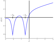
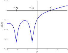
(a)	(b)

Figure 1. Plot of the secular function $\phi(\sigma)$ given in (13). (a) The case when $\phi(0)\geq 0$, which implies that the unconstrained minimizer of (4) is feasible. (b) When $\phi(0)<0$, there exists $\sigma^{*}>0$ such that $\phi(\sigma^{*})=0$, i.e., $v^{*}=-(\Lambda+\sigma^{*}I)^{-1}\tilde{g}$ is well-defined and is feasible.

The method to obtain $\sigma^{*}$ is significantly different that the one used in [20] in that we explicitly use the eigendecomposition within Newton’s method to compute the optimal $\sigma^{*}$. That is, we differentiate the reciprocal of $\|v(\sigma)\|$ in (14) to compute the derivative of $\phi(\sigma)$ in (13), obtaining a Newton update that is expressed only in terms of $g_{\parallel}$, $g_{\perp}$, and the eigenvalues of $B$. In contrast to [20], this approach eliminates the need for matrix solves for each Newton iteration (see Alg. 2 in [20]).

Given $\sigma^{*}$ and $v^{*}$, the optimal $p^{*}$ is obtained as follows. Letting $\tau^{*}=\gamma+\sigma^{*}$, the solution to the first optimality condition, $(B+\sigma^{*}I)p^{*}=-g,$ is given by

$$p^{*} = -(B+\sigma^{*}I)g$$ (15)

$$= -(\gamma I+\Psi M\Psi^{T}+\sigma^{*}I)^{-1}g$$

$$= -\frac{1}{\tau^{*}}\left[I-\Psi(\tau^{*}M^{-1}+\Psi^{T}\Psi)^{-1}\Psi^{T}\right]g,$$

using the Sherman-Morrison-Woodbury formula. Algorithm 1 details the proposed approach for solving the trust-region subproblem.

Algorithm 1: L-BFGS Trust-Region Subproblem Solver

Compute $R$ from the “thin” QR factorization of $\Psi$;

Compute the spectral decomposition

  $RMR^{T}=V\hat{\Lambda}V^{T}$ with $\hat{\lambda}_{1}\leq\hat{\lambda}_{2}\leq\cdots\leq\hat{\lambda}_{2(k+1)}$;

Let $\Lambda_{1}=\hat{\Lambda}+\gamma I$;

Define $P_{\parallel}=\Psi R^{-1}V$ and $g_{\parallel}=P_{\parallel}^{T}g$;

Compute $\|g_{\perp}\|_{2}=\sqrt{\|g\|_{2}^{2}-\|g_{\parallel}\|_{2}^{2}}$;

if $\phi(0)\geq 0$ then

 $\sigma^{*}=0$ and compute $p^{*}$ from (15) with $\tau^{*}=\gamma$;

else

 Use Newton’s method to find $\sigma^{*}$;

 Compute $p^{*}$ from (15) with $\tau^{*}=\gamma+\sigma^{*}$;

end

Algorithm 2 outlines our overall limited-memory L-BFGS trust-region approach.

Algorithm 2: TrustSpa: Limited-Memory BFGS Trust-Region Method for Sparse Relaxation

Define parameters: $m$, $0<\tau_{1}<0.5$, $0<\varepsilon$;

Initialize $x_{0}\in\mathbb{R}^{n}$ and compute $g_{0}=\nabla\Phi(z_{0})$;

Let $k=0$;

while not converged

 if $\|g_{k}\|_{2}\leq\varepsilon$ then done

 Use Algorithm 1 to find $p_{k}$ that solves (2);

 Compute $\rho_{k}=(f(z_{k}+p_{k})-f(z_{k}))/q_{k}(p_{k})$;

 Compute $g_{k+1}$ and update $B_{k+1}$;

 if $\rho_{k}\geq\tau_{1}$ then

  $z_{k+1}=z_{k}+p_{k}$;

 else

  $z_{k+1}=z_{k};$

 end if

 Compute trust-region radius $\delta_{k+1}$;

 $k\leftarrow k+1$;

end while

The method described here guarantees that the trust-region subpoblem is solved to high accuracy. Other quasi-Newton trust-region methods for L-BFGS matrices that solve to high accuracy include [21], which uses a shifted L-BFGS approach, and [22], which uses a “shape-changing” norm in (2).

5. NUMERICAL EXPERIMENTS

We call the proposed method, Trust-Region Method for Sparse Relaxation (TrustSpa Relaxation, or simply TrustSpa). We evaluate its effectiveness by reconstructing a sparse signal from Gaussian noise corrupted low-dimensional measurements. In this experiment, the true signal $f$ is of size 4,096 with 160 randomly assigned nonzeros with amplitude $\pm 1$ (see Fig. 2(a)). We obtain compressive measurements $y$ of size 1,024 (see Fig. 2(b)) by projecting the true signal using a randomly generated system matrix ($A$) from the standard normal distribution with orthonormalized rows. In particular, the measurements are corrupted by 5% of Gaussian noise.

(a) Truth $f$ ($\tilde{n}=4096$, number of nonzeros = 160)

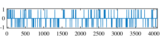
(b) Measurements $y$ ($\tilde{m}=1024$, noise level = 5% )

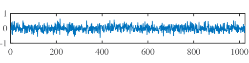
Figure 2. Experimental setup: (a) True signal $f$ of size 4,096 with 160 $\pm$ spikes, (b) compressive measurements $y$ ($\tilde{m}=1024$) with 5% Gaussian noise.

We implemented TrustSpa in MATLAB R2015a using a PC with Intel Core i7 2.8GHz processor with 16GB memory. We compared the performance of TrustSpa with the Gradient Projection for Sparse Reconstruction (GPSR) method [4] with the Barzilai and Borwein (BB) approach [23] and without the debiasing option. Both TrustSpa and GPSR-BB methods are initialized at the same starting point, i.e., zero and terminate if the relative objective values do not significantly change, i.e, $|\Phi(x^{k+1})-\Phi(x^{k})|/|\Phi(x^{k})|\leq 10^{-8}$. The regularization parameter $\tau$ in (1) is optimized independently for each algorithm to minimize the mean-squared error (MSE = $\tfrac{1}{n}\|\hat{f}-f\|_{2}^{2}$, where $\hat{f}$ is an estimate of $f$).

(a) GPSR-BB reconstruction $\hat{f}_{\text{GPSR}}$ (MSE = 1.624e-04)

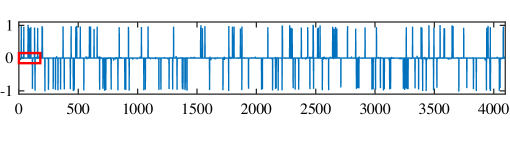
(b) TrustSpa reconstruction $\hat{f}_{\text{TS}}$ (MSE = 9.347e-05)

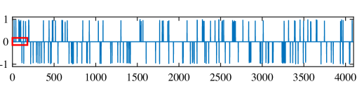
Figure 3. (a) GPSR-BB reconstruction, $\hat{f}_{\text{GPSR}}$, (b) TrustSpa reconstruction, $\hat{f}_{\text{TS}}$. MSE = $(1/n)\|\hat{f}-f\|_{2}^{2}$. Note the lower MSE for the proposed method.

Analysis. We ran the experiment 10 times with 10 different Gaussian noise realizations. The average MSE for GPSR-BB for the 10 trials is $1.758\times 10^{-4}$ and the average computational time is 4.45 seconds. In comparison, the average MSE for TrustSpa is $9.827\times 10^{-5}$, and the average computational time is 3.52 seconds. For one particular trial, the GPSR-BB reconstruction, $\hat{f}_{\text{GPSR}}$ (see Fig. 3(a)), has MSE $1.624\times 10^{-4}$ while the TrustSpa reconstruction, $\hat{f}_{\text{TS}}$ (see Fig. 3(b)), has MSE $9.347\times 10^{-5}$. Note that the $\hat{f}_{\text{TS}}$ has fewer reconstruction artifacts (see Fig. 4). Quantitatively, $\hat{f}_{\text{GPSR}}$ has 786 nonzeros, where the spurious solutions are between the order of $10^{-2}$ and $10^{-3}$. In contrast, because of the variable transformations used by TrustSpa, the algorithm terminates with no zero components in its solution; however, only 579 components are greater than $10^{-6}$ in absolute value. This has the effect of rendering most spurious solutions less visible.

(a) Zoomed region of $\hat{f}_{\text{GPSR}}$

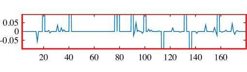
(b) Zoomed region of $\hat{f}_{\text{TS}}$

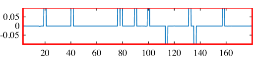
Figure 4. Zoomed red-boxed regions in the reconstructions: (a) A zoomed region of $\hat{f}_{\text{GPSR}}$, (b) a zoomed region of $\hat{f}_{\text{TS}}$. Note the presence of artifacts in the GPSR-BB reconstruction that are absent in the proposed method’s reconstruction.

6. CONCLUSION

In this paper, we proposed an approach for solving the $\ell_{2}$-$\ell_{1}$ minimization problem that arises in compressed sensing and sparse recovery problems. Unlike gradient projection-type methods like GPSR, which uses only the current gradient, our approach uses gradients from previous iterations to obtain a more accurate Hessian approximation. Numerical experiments show that our proposed approach mitigates spurious solutions more effectively with a lower average MSE in a smaller amount of time.

References

- [1] R. Tibshirani, “Regression shrinkage and selection via the lasso,” J. Roy. Statist. Soc. Ser. B, vol. 58, no. 1, pp. 267–288, 1996.
- [2] E. J. Candès and T. Tao, “Decoding by linear programming,” IEEE Trans. Inform. Theory, vol. 15, no. 12, pp. 4203–4215, 2005.
- [3] D. L. Donoho, “Compressed sensing,” IEEE Trans. Inform. Theory, vol. 52, no. 4, pp. 1289–1306, 2006.
- [4] M.A.T. Figueiredo, R.D. Nowak, and S.J. Wright, “Gradient projection for sparse reconstruction: Application to compressed sensing and other inverse problems,” IEEE Journal of Selected Topics in Signal Processing, vol. 1, no. 4, pp. 586–597, 2007.
- [5] A. Banerjee, S. Merugu, I. S. Dhillon, and J. Ghosh, “Clustering with Bregman divergences,” The Journal of Machine Learning Research, vol. 6, pp. 1705–1749, 2005.
- [6] A. Oh and R. Willett, “Regularized non-Gaussian image denoising,” ArXiv Preprint 1508.02971, 2015.
- [7] J. Yu, S.V.N. Vishwanathan, S. Günter, and N. N. Schraudolph, “A quasi-Newton approach to nonsmooth convex optimization problems in machine learning,” The Journal of Machine Learning Research, vol. 11, pp. 1145–1200, 2010.
- [8] J. Lee, Y. Sun, and M. Saunders, “Proximal Newton-type methods for convex optimization,” in Advances in Neural Information Processing Systems, 2012, pp. 836–844.
- [9] G. Zhou, X. Zhao, and W. Dai, “Low rank matrix completion: A smoothed l0-search,” in 2012 50th Annual Allerton Conference on Communication, Control, and Computing (Allerton). IEEE, 2012, pp. 1010–1017.
- [10] S. Becker and J. Fadili, “A quasi-newton proximal splitting method,” in Advances in Neural Information Processing Systems, 2012, pp. 2618–2626.
- [11] Y. Wang, J. Cao, and C. Yang, “Recovery of seismic wavefields based on compressive sensing by an l1-norm constrained trust region method and the piecewise random subsampling,” Geophysical Journal International, vol. 187, no. 1, pp. 199–213, 2011.
- [12] M. Hintermüller and T. Wu, “Nonconvex TVq-models in image restoration: Analysis and a trust-region regularization–based superlinearly convergent solver,” SIAM Journal on Imaging Sciences, vol. 6, no. 3, pp. 1385–1415, 2013.
- [13] D. M. Gay, “Computing optimal locally constrained steps,” SIAM J. Sci. Statist. Comput., vol. 2, no. 2, pp. 186–197, 1981.
- [14] J. J. Moré and D. C. Sorensen, “Computing a trust region step,” SIAM J. Sci. and Statist. Comput., vol. 4, pp. 553–572, 1983.
- [15] A. R. Conn, N. I. M. Gould, and P. L. Toint, Trust-Region Methods, Society for Industrial and Applied Mathematics (SIAM), Philadelphia, PA, 2000.
- [16] D. C. Liu and J. Nocedal, “On the limited memory BFGS method for large scale optimization,” Math. Program., vol. 45, pp. 503–528, 1989.
- [17] J. Nocedal and S. Wright, Numerical optimization, Springer Science & Business Media, 2006.
- [18] I. Griva, S. G. Nash, and A. Sofer, Linear and nonlinear programming, Society for Industrial and Applied Mathematics, Philadelphia, 2009.
- [19] R. H. Byrd, J. Nocedal, and R. B. Schnabel, “Representations of quasi-Newton matrices and their use in limited-memory methods,” Math. Program., vol. 63, pp. 129–156, 1994.
- [20] J. V. Burke, A. Wiegmann, and L. Xu, “Limited memory BFGS updating in a trust-region framework,” Technical report, University of Washington, 1996.
- [21] J. B. Erway and R. F. Marcia, “Algorithm 943: MSS: MATLAB software for L-BFGS trust-region subproblems for large-scale optimization,” ACM Transactions on Mathematical Software, vol. 40, no. 4, pp. 28:1–28:12, June 2014.
- [22] O. Burdakov, L. Gong, Y.-X. Yuan, and S. Zikrin, “On efficiently combining limited memory and trust-region techniques,” Tech. Rep. 2013:13, Link ping University, Optimization, 2015.
- [23] J. Barzilai and J. M. Borwein, “Two-point step size gradient methods,” IMA Journal of Numerical Analysis, vol. 8, no. 1, pp. 141–148, 1988.