Operators for Space and Time in BeSpaceD

Abstract

In this report, we present some spatio-temporal operators for our BeSpaceD framework. We port operators known from functional programming languages such as filtering, folding and normalization on abstract data structures to the BeSpaceD specification language. We present the general ideas behind the operators, highlight implementation details and present some simple examples.

1 Introduction

This report continues our work on BeSpaceD by introducing new operators for filtering, folding and normalization of BeSpaceD descriptions. The new operators are inspired by operations from functional programming languages and are applied to spatio-temporal models.

BeSpaceD is our framework for spatio-temporal reasoning [4, 5]. BeSpaceD is characterised by

• A description language that is based on abstract datatypes.

• Means to reason about descriptions formulated in the description language.

Related work comprises process algebra based formalisms [9, 10] and [12]. Similar to this work, we have created a formal specification language as part of our BeSpaceD framework. In our case, specifications are instances of abstract datatypes and follow a more functional programming style. Further related is work on type systems in connection with this process algebra work that has been introduced in [8]. Analog to the work presented in [8], BeSpaceD can also be used to define spatio-temporal types. A verification tool to check properties based on the process algebra inspired formalism is described in [11]. Applications include concurrency and ressource control. Further related are approaches for the specification of hybrid systems. A framework for specifying hybrid programs with stochastic features is presented in [20]. Other logic approaches to spatial reasoning can be found, e.g., in [16, 1, 21]. Specialised solutions for reasoning about geometric constraints have been developed for robot path planning. This area has already been studied for decades, see e.g., [18, 17].

This report provides an overview on BeSpaceD in Section 2. Filtering is covered in Section 3. Folding of time and space is covered in Section 4 while normalization is described in Section 5. Section 6 concludes the report.

2 BeSpaceD

BeSpaceD is a spatio-temporal modeling and reasoning framework. Here, we describe the modeling language, BeSpaceD-based reasoning, and provide some implementation background information.

2.1 BeSpaceD-based Modeling

BeSpaceD is implemented in Scala. Its core functionality runs in a Java environment. In the past, we have successfully applied BeSpaceD in different contexts such as decision support for factory automation [6, 7], coverage analysis for mobile devices [14] and for verification of spatio-temporal properties for industrial robots [15, 13, 3].

BeSpaceD models are created using Scala case classes. Thus, we provide a functional abstract datatype-like feeling. Major language constructs which are currently available (see also [2]) are provided below. An Invariant is the basic logical entity, something that is supposed to hold for a system throughout space and time. Invariants can and typically do, however, contain conditional parts, something that requires a precondition to hold, e.g., a certain time implies a certain state of a system. Constructors for basic logical operations connect invariants to form a new invariant. Some of these basic constructors are provided below:

abstract class Invariant;

abstract class ATOM extends Invariant;

case class OR (t1 : Invariant, t2 : Invariant) extends Invariant;
case class AND (t1 : Invariant, t2 : Invariant)  extends Invariant;
case class NOT (t : Invariant) extends Invariant;
case class IMPLIES (t1 : Invariant, t2 : Invariant)  extends Invariant;

case class BIGOR (t : List[Invariant]) extends Invariant;
case class BIGAND (t : List[Invariant]) extends Invariant;

case class TRUE() extends ATOM;
case class FALSE() extends ATOM;

Additional predicates are used to indicate timepoints, timeintervals, events, ownership, and related information.

...
case class TimePoint [T] (timepoint : T) extends ATOM;
case class TimeInterval [T](timepoint1 : T, timepoint2 : T) extends ATOM;
...
case class Event[E] (event : E) extends ATOM;
case class Owner[O] (owner : O) extends ATOM;
case class Prob (probability : Double) extends ATOM;
case class ComponentState[S] (state : S) extends ATOM;

Some geometric constructs are provided below:

case class OccupyBox (x1 : Int,y1 : Int,x2 : Int,y2 : Int) extends ATOM;
case class OccupyBoxSI (x1 : SI,y1 : SI,x2 : SI,y2 : SI) extends ATOM;
case class EROccupyBox
   (x1 : (ERTP => Int),y1 : (ERTP => Int),
    x2 : (ERTP => Int),y2 : (ERTP => Int)) extends ATOM;
case class OwnBox[C] (owningcomponent : C,x1 : Int,y1 : Int,x2 : Int,y2 : Int)
            extends ATOM;
...
case class Occupy3DBox (x1 : Int, y1: Int, z1 : Int,
             x2 : Int, y2 : Int, z2 : Int) extends ATOM;
...
case class OccupyPoint (x:Int, y:Int) extends ATOM
case class OwnPoint[C] (owningcomponent : C,x:Int, y:Int) extends ATOM

case class Occupy3DPoint (x:Int, y:Int, z: Int) extends ATOM
...
case class OccupyCircle (x1 : Int, y1 : Int, radius : Int) extends ATOM;
case class OwnCircle[C] (owningcomponent : C,
             x1 : Int, y1 : Int, radius : Int) extends ATOM;
...

In addition, we have topological constructs which are shown below:

case class OccupyNode[N] (node : N) extends ATOM
...
case class Edge[N] (source : N, target : N) extends ATOM
case class Transition[N,E] (source : N, event : E, target : N) extends ATOM

In summary, the language constructs comprise basic logical operators (e.g., AND, OR) and constructs for space, time, and topology. For instance, OccupyBox refers to a rectangular two-dimensional geometric space. It is parameterized by its left lower and its right upper corner points. An example is provided below: if we want to express that the rectangular space with the corner points $(42,3056)$ and $(1531,2605)$ is subject to a semantic condition “A” between integer-defined time points $100$ and $150$, we may use the following BeSpaceD formula:

...
  IMPLIES(AND(TimeInterval(100,150),
               Owner("A")),
      OccupyBox(42,3056,1531,2605))
...

2.2 BeSpaceD-based Reasoning

BeSpaceD comes with a variety of library-like functionality that involves the handling of specifications. BeSpaceD formulas can be efficiently analyzed, i.e., verifying spatio-temporal and other properties. A simple example involves the specification of a point in time and a predicate. BeSpaceD can derive the spatial implications from these definitions. We have implemented algorithms and connected tools such as an external SMT solvers (e.g., we have a connection to z3 [19]). These can help to resolve geometric constraints such as overlapping of different areas in time and space. Different operators (for instance, breaking geometric constraints on areas down to geometric constraints on points) exist. In this report, we are looking at filtering in datatypes, normalization and spatio-temporal fold operations. Filtering and normalization were already supported in previous versions but have seen some updates in the implementation. The folding functionality is new to this report.

2.3 Implementation

In the implementation of the presented operations we are using the Scala programming language. In particular Scala’s case classes are used to define the language and we make heavy use of pattern matching on types to implement algorithms. For unit testing we use ScalaTest  which allows us to easily code tests with assertions and rapidly re-run them as needed. The team used a combination of the Eclipse “Scala IDE” (mostly for runtime execution) and IntelliJ IDEA  (mostly for for editing and refactoring).

3 Filtering

Filtering allows the selection of relevant information out of larger BeSpaceD invariants thereby returning a sub-invariant.

Filter functions have the following signiture scheme:

filter(inv : Invariant,filtercondition) : Invariant

An invariant is filtered following a filtercondition. The filter condition may be a spatial area or a timeinterval. All relevant information for the filtercondition is encapsulated in the returned invariant.

A variety of different filter functions are possible, each one evaluating the invariant with respect to different levels of semantic depth.

Implementation

As part of the implementation of a fold, a filter function is required. To illustrate one interesting example of this we will discuss the filterTime function. Presented below is one of our versions of filtering time which is of particular interest because it uses an elegant ”rewrite then simplify” algorithm that greatly reduces the code complexity compared to other versions of filterTime. However, we did not perform an analysis of algorithmic complexity so far.

The key line of source code is:

case tp: TimePoint[IntegerTime] =>
           if (withinTimeWindow(tp, startTime, stopTime)) tp
           else successReturn.not

This line rewrites the time point predicate as either a true or false value. ”tp” effects no change to the invariant and ”successReturn.not” will rewrite it as either a TRUE or FALSE value. This depends on the parent context of the re-write: FALSE for conjunctions and TRUE for disjunctions. Later in the simplification process:

  simplifyInvariant(filteredInvariant)

will cause whole branches of the abstract datatype tree to be truncated where the time point is rewritten as false because one of the standard simplification rules is:

  case IMPLIES(FALSE(),t2) => TRUE()

In effect this filters out all the sub expressions that do not match the desired time point. Other aspects of the source code can be found below:

  def filterTime2(startTime: IntegerTime,
                  stopTime: IntegerTime,
                  successReturn: BOOL)
                     (invariant: Invariant): Invariant =
  {
    val filter = filterTime2(startTime, stopTime, successReturn) _

    def withinTimeWindow(timePoint: TimePoint[IntegerTime],
                         startTimeInclusive: IntegerTime,
                         stopTimeExclusive: IntegerTime): Boolean =
    {
      val time = timePoint.timepoint

      time >= startTimeInclusive && time < stopTimeExclusive
    }

    val filteredInvariant: Invariant = invariant match
    {
      case tp: TimePoint[IntegerTime] =>
                 if (withinTimeWindow(tp, startTime, stopTime)) tp
                 else successReturn.not

      case IMPLIES(premise, conclusion) =>
              IMPLIES(filter(premise), filter(conclusion))

      case AND(t1, t2) => AND(filter(t1), filter(t2))
      case BIGAND(sublist) => BIGAND(sublist map filter)

      case OR(t1, t2) => OR( filter(t1), filter(t2) )
      case BIGOR(sublist) => BIGOR(sublist map filter)

      case other => other
    }

    simplifyInvariant(filteredInvariant)
  }

4 Folding

Figure 1 shows an illustration of our fold operation for time and space. The general principle of folding, the iteration through time and space while accumulating processed information is shown.

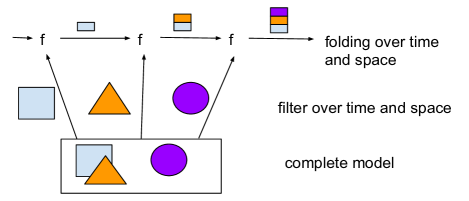
Figure 1: Fold operator for space and time

In this section, we discuss the folding of time and space in separate subsections and follow our implementation.

4.1 Time

A generalized signature for a folding time function is provided below. No assumptions are made on the implementation of time, other than that time has to be partially ordered.

foldTime[A,T] (invariant : Invariant, a: A,starttime : T,
                       stoptime : T,step: T, f [A -> Invariant -> A])

Implementation

We are exemplifying the folding of time by using an example with weather data. We are regarding a geometric space (a matrix-like structure) that contains values indicating cloud coverage of an area. To validate folding time we devised a complex test case that aggregates clouded areas over multiple time points. This test case uses a naive approach as it requires a strict format for the knowledge invariants. The knowledge about the space and whether its cloudy or not is encoded as follows:

// Time
val t1 = new IntegerTime(1)
val t2 = new IntegerTime(2)
val t3 = new IntegerTime(3)

// Overlapping Boxes
val b1 = OccupyBox(1, 1, 10, 10) // Area 100
val b2 = OccupyBox(5, 5, 15, 15) // Area 121
val b3 = OccupyBox(10, 10, 20, 20) // Area 121

// Time occupied
val to1 = IMPLIES(TimePoint(t1), b1)
val to2 = IMPLIES(TimePoint(t2), b2)
val to3 = IMPLIES(TimePoint(t3), b3)

val timeSeries = List(to1, to2, to3)
val conjunction = BIGAND(timeSeries)

In order to calculate the area occupied for one time step we implemented a function called addAreaOccupied. This function takes two parameters:

1. total: This is called the accumulator as it will store the running total (an Integer) as the fold is being called recursively.

2. item: This is BeSpaceD data (an invariant) that represents the knowledge of the spatial cloud system.

def calculateArea(box: OccupyBox): Int =
   Math.abs((box.x2 - box.x1 + 1) * (box.y2 - box.y1 + 1))

def addAreaOccupied(total: Int, item: Invariant): Int = {
  val area = item match {
    case IMPLIES(imp, box: OccupyBox) => calculateArea(box)
    case _ => 0
  }

  total + area
}

It is interesting to note that the result of this function is a calculation derived from the two parameters (as seen in the last line above). In this case the accumulator (total) is added to the area which is calculated from the second parameter (item). This is the essence of an ”aggregation function” that is commonly used by all fold operations: The accumulated value and a function applied to the next iteration item are combined to give the next accumulated value.

The signature for an implemented function that folds time is as follows:

  def foldTime[A](
                   invariant: Invariant,
                   accumulator: A,
                   startTime: IntegerTime,
                   stopTime: IntegerTime,
                   step: IntegerTime.Step,
                   f: (A, Invariant) => A
                   ): A

Additionally, for our example, we need to setup a few more parameters. The accumulator used in the fold needs an initial value:

val initialValue = 0

And finally we need to define a series of “steps” in time for the fold operation to “fold”. In this test case we specified the following:

t1, t3, 1

This series of values simply represents start with time point 1, stop at time point 3 and step through time incrementing by 1.

Here is what the call to the foldTime function with the parameters described above looks like:

val foldedTime = foldTime[Int](
  conjunction,
  initialValue,
  t1, t3, 1,
  addAreaOccupied
)

To validate the test runs correctly we assert the expected result:

assertResult(expected = 342)(actual = foldedTime)

The expected result of 342 is explained as follows: There are three time points: 1, 2 and 3 each with their own boxes: b1, b2, b3. The area of each are 100, 121, 121. The fold of these three areas will be the sum which is 342.

The actual fold over time example is also depicted in Figure 2. The regarded spatial area stays the same, but the cloud moves over time (depicted in different colors).

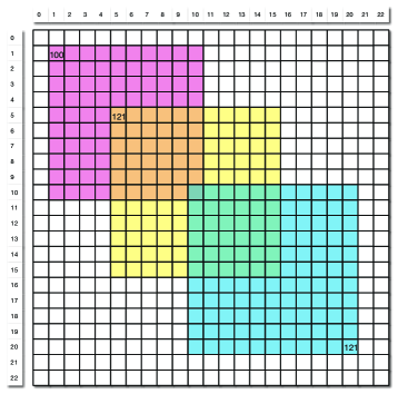
Figure 2: Fold over time illustrated

4.2 Space

Folding space in general is done by using a function with the following signature. Note, that it works using generic area descriptions.

foldSpace[A] (
    invariant: Invariant,
    z: A, startarea: Invariant,
    stoparea: Invariant,
    stepareaOrBox: Invariant,
    f: (A -> Invariant -> A))

Implementation

A concrete signature for an implemented function that folds space is as follows and assumes that areas are boxes:

foldSpace[A](
                  invariant: Invariant,
                  accumulator: A,
                  startArea: OccupyBox,
                  stopArea: OccupyBox,
                  translation: Translation,
                  f: (A, Invariant) => A
                  ): A

To validate folding space we devised a simple test case that aggregates clouded areas over multiple spatial iteration steps. This test case uses a naive approach as it requires a strict format for the knowledge invariants. The knowledge about the space and whether its cloudy or not is encoded as follows:

    // Boxes
    val b1 = OccupyBox(1, 1, 10, 10)
    val b2 = OccupyBox(5, 5, 15, 15)
    val b3 = OccupyBox(10,10, 20,20)
    val b4 = OccupyBox(21,21, 30,30)

    // Space owner-occupied
    val s1 = IMPLIES(mountain, b1)
    val s2 = IMPLIES(cloud, b2)
    val s3 = IMPLIES(cloud, b3)
    val s4 = IMPLIES(mountain, b4)

    val spaceSeries = List(s1, s2 , s3, s4)
    val conjunction = BIGAND(spaceSeries)

In order to apply the foldSpace function we need to pass in the calculateArea function from the above example as the parameter f and a spatial model as the invariant.

Additionally we need to setup a few more parameters. The accumulator using in the fold needs an initial value:

val initialValue = 0

And finally we need to define a series of steps in space for the fold operation to “fold”. In this test case we defined the following:

    val startBox = OccupyBox(1, 1, 5, 5)
    val stopBox  = OccupyBox(26,26,30,30)
    val step: Translation = (5, 5)

This means we want the first box cover coordinates: (1,1) … (1,5), (2,1) … (2,5) … (5,5). In this example there are six iteration steps none of which overlap. In addition, as future work we would like to regard overlapping steps and explore semantic implications for this.

The code piece below shows a call to the foldSpace function with the parameters described above:

    val foldedSpace = foldSpace[Int](
      normalisedData,
      initialValue,
      startBox, stopBox, step,
      addCloudyArea
    )

To validate the test runs we assert the expected result using the following code line:

    assertResult(expected = 76)(actual = foldedSpace)

The expected result on 76 is explained as follows:

The first iteration box (1,1 … 5,5) is indicated to contain a mountain (see above). However, one point also contains a cloud. This point is counted for cloud coverage. We further iterate through the boxes. The second iteration box (6,6 … 10,10) is indicated to contain a cloud. We continue iterating through the iteration path thereby examining all 6 boxes in the path. The total cloud covered area in the iteration path adds up to 1 + 25 + 25 + 25 + 0 + 0= 76.

In order to calculate a “degree of cloudiness” for one spatial step we implemented a function called addCloudyArea. This function takes two parameters:

1. total: This is called the accumulator as it will store the running total (an Integer) as the fold is being called recursively.

2. invariant: This is BeSpaceD data that represents the model containing clouds and other spatio-temporal information.

def addCloudyArea(total: Int, invariant: Invariant): Int =
{
  def isCloudyArea(owner: Owner[Any]): Boolean = owner == cloud

  def calculateArea(list: List[Invariant]): Int = {
    val areas: List[Int] = list map {
      inv: Invariant =>
        inv match {
          case IMPLIES(owner: Owner[Any], point: OccupyPoint) =>
             if (isCloudyArea(owner)) 1 else 0
          case IMPLIES(owner: Owner[Any],
                       AND(p1: OccupyPoint, p2: OccupyPoint)) =>
             if (isCloudyArea(owner)) 2 else 0
          case IMPLIES(owner: Owner[Any],
                       BIGAND(points: List[OccupyPoint])) =>
             if (isCloudyArea(owner)) points.length else 0
          case _ => 0
        }
    }
    areas.sum
  }

  val area = invariant match {
    case AND(t1, t2) => calculateArea(t1 :: t2 :: Nil)
    case BIGAND(sublist: List[Invariant]) => calculateArea(sublist)
    case _ => 0
  }

  total + area
}

It is interesting to note that the result of this function is a calculation derived from the two parameters (as seen in the last line above). In this case the accumulator (total) is added to the area which is calculated from the second parameter (invariant).

The folding of space example is also illustrated in Figure 3. Different boxes are shown for the different steps in our example.

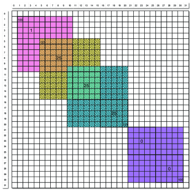
Figure 3: Folding space example illustrated

5 Normalization

In order to make invariants comparable, we need to normalize them. Normalization ensures, that the same invariants are represented in the same way. However, there are different levels of normalization. Normalization can take a higher or lower degree of semantics into account. At the lower end, we may just reorder arguments for logical operators such as “and” and “or”. On the other end, we may look into the semantic meaning of geometric shapes and, e.g., replace areas with sets of points in order to make them comparable. Different normalization strategies may require different resources and work on different subsets of our language. Choosing an appropriate form of normalization depends on the actual use-case. This is why we have not implemented a single normalization function, but rather have a family of functions.

In general normalization involves term rewriting steps until a fix point is reached. The invariant is then in a normal form. Several properties of the term rewriting should be fulfilled such as confluence. Comparison is then carried out by checking the resulting terms for equality.

Implementation

To implement normalization in BeSpaceD we used functional composition in chains. The type of each element in the chain is a function from Invariant to Invariant:

type Processor[I, O] = I => O
type InvariantProcessor = Processor[Invariant, Invariant]

We have created various invariant processors each of which perform one step in the normalisation process. The following is a general normalization function, showing the composition of four processors:

val normalize: InvariantProcessor =
     flatten
     compose
     order
     compose
     deduplicate
     compose
     simplify

A more specific example of a normalization function designed for data of the form

Owner >  OccupyPoints

is described in the following. It composes the standard normalization with a further processor specific to the data structure.

val normalizeOwnerOccupied: InvariantProcessor = mergeOwners compose
normalize

Below is a brief description of the step each processor does in the normalization process:

• flatten – rewrites nested conjunctions and disjunctions into single level conjunctions and disjunctions where possible.

• order – orders the terms of all conjunctions and disjunctions according to a standard ordering.

• deduplicate – removes duplicate terms of conjunctions and disjunctions.

• simplify – uses term rewriting to rewrite expressions in a simpler form. e.g. IMPLIES(TRUE, t2) is rewritten as t2

• mergeOwners - expects a BIGAND of IMPLIES and conjuncts all the conclusions of implications that have identical premises. e.g.

  BIGAND(IMPLIES(A, X), IMPLIES(B, Y), IMPLIES(A, Z))
  

  is rewritten as

  BIGAND(IMPLIES(A, AND(X, Z)), IMPLIES(B, Y))
  

6 Conclusion

We presented new operators for BeSpaceD in this paper. These operators comprise filtering, folding and normalization for spatio-temporal formulas. The operations are inspired by functional programming languages and are ported to the spatio-temporal context. In addition to theoretical considerations we presented an implementation and a testing infrastructure for the BeSpaceD framework.

Acknowledgement

The implementation work presented in this paper is open source and freely available. It has been done as part of the research and development activities in the Australia-India Centre for Automation Software Engineering at RMIT University in Melbourne.

References

- [1] B. Bennett, A. G. Cohn, F. Wolter, M. Zakharyaschev. Multi-Dimensional Modal Logic as a Framework for Spatio-Temporal Reasoning. Applied Intelligence, Volume 17, Issue 3, Kluwer Academic Publishers, November 2002.
- [2] J. O. Blech. An Example for BeSpaceD and its Use for Decision Support in Industrial Automation. ArXiv e-prints, 1512.04656, Dec. 2015.
- [3] J. O. Blech and Peter Herrmann. Behavioral Types for Space-aware Systems. Model-based Architecting of Cyber-Physical and Embedded Systems. CEUR proceedings, vol. 1508, 2015.
- [4] J. O. Blech and H. Schmidt. BeSpaceD: Towards a Tool Framework and Methodology for the Specification and Verification of Spatial Behavior of Distributed Software Component Systems. In arXiv.org, http://arxiv.org/abs/1404.3537, 2014.
- [5] J. O. Blech and H. Schmidt. Towards Modeling and Checking the Spatial and Interaction Behavior of Widely Distributed Systems. In Improving Systems and Software Engineering Conference, 2013.
- [6] J. O. Blech, I. Peake, H. Schmidt, M. Kande, S. Ramaswamy, Sudarsan SD., and V. Narayanan. Collaborative Engineering through Integration of Architectural, Social and Spatial Models. Emerging Technologies and Factory Automation (ETFA), IEEE, 2014.
- [7] J. O. Blech, I. Peake, H. Schmidt, M. Kande, A. Rahman, S. Ramaswamy, Sudarsan SD., and V. Narayanan. Efficient Incident Handling in Industrial Automation through Collaborative Engineering. Emerging Technologies and Factory Automation (ETFA), IEEE, 2015.
- [8] L. Caires. Spatial-behavioral types for concurrency and resource control in distributed systems. Theoretical Computer Science, Elsevier, 2008.
- [9] L. Caires and L. Cardelli.A Spatial Logic for Concurrency (Part I). Information and Computation, Vol 186/2 November 2003.
- [10] L. Caires and L. Cardelli. A Spatial Logic for Concurrency (Part II). Theoretical Computer Science, 322(3) pp. 517-565, September 2004.
- [11] L. Caires and H. Torres Vieira. SLMC: a tool for model checking concurrent systems against dynamical spatial logic specifications. Tools and Algorithms for the Construction and Analysis of Systems. Springer, 2012.
- [12] S. Haar, S. Perchy, C. Rueda, F. Valencia. An Algebraic View of Space/Belief and Extrusion/Utterance for Concurrency/Epistemic Logic. Principles and Practice of Declarative Programming, 2015.
- [13] F. Han, J. O. Blech, P. Herrmann, H. Schmidt. Towards Verifying Safety Properties of Real-Time Probabilistic Systems. Formal Engineering approaches to Software Components and Architectures, 2014.
- [14] F. Han, J. O. Blech, P. Herrmann, H. Schmidt. Model-based Engineering and Analysis of Space-aware Systems Communicating via IEEE 802.11. COMPSAC, IEEE, 2015.
- [15] P. Herrmann, J. O. Blech, F. Han, and H. Schmidt. A Model-based Toolchain to Verify Spatial Behavior of Cyber-Physical Systems. Asia-Pacific Services Computing Conference (APSCC), 2014.
- [16] D. Hirschkoff, É. Lozes, D. Sangiorgi. Minimality Results for the Spatial Logics. Foundations of Software Technology and Theoretical Computer Science, vol 2914 of LNCS, Springer, 2003.
- [17] J-C. Latombe. Robot Motion Planning. Kluwer Academic Publishers, 1991.
- [18] S. Kambhampati and L.S. Davis. Multiresolution path planning for mobile robots. Volume 2 , Issue: 3, Journal of Robotics and Automation, IEEE 1986.
- [19] L. De Moura, N. Bjørner. Z3: An efficient SMT solver. In Tools and Algorithms for the Construction and Analysis of Systems (pp. 337-340). Springer, 2008.
- [20] A. Platzer. Stochastic differential dynamic logic for stochastic hybrid programs. In Automated Deduction, CADE-23 (pp. 446-460). Springer, Berlin Heidelberg 2011.
- [21] S. Dal Zilio, D. Lugiez, C. Meyssonnier. A logic you can count on. Symposium on Principles of programming languages, ACM, 2004.