Cache Size Allocation in Backhaul Limited Wireless Networks

Abstract

Caching popular content at base stations is a powerful supplement to existing limited backhaul links for accommodating the exponentially increasing mobile data traffic. Given the limited cache budget, we investigate the cache size allocation problem in cellular networks to maximize the user success probability (USP), taking wireless channel statistics, backhaul capacities and file popularity distributions into consideration. The USP is defined as the probability that one user can successfully download its requested file either from the local cache or via the backhaul link. We first consider a single-cell scenario and derive a closed-form expression for the USP, which helps reveal the impacts of various parameters, such as the file popularity distribution. More specifically, for a highly concentrated file popularity distribution, the required cache size is independent of the total number of files, while for a less concentrated file popularity distribution, the required cache size is in linear relation to the total number of files. Furthermore, we study the multi-cell scenario, and provide a bisection search algorithm to find the optimal cache size allocation. The optimal cache size allocation is verified by simulations, and it is shown to play a more significant role when the file popularity distribution is less concentrated.

I Introduction

The demand for mobile data is continuously increasing, which results from the prevalence of smart devices, as well as subscribers’ desire for high-quality and low-latency services, such as high definition (HD) video on demand. It is predicted that global cellular data traffic will increase nearly tenfold in the next five years, and around 75 percent of the world’s mobile data traffic will be video by 2019 [1]. Such rapid growth has been driving operators to provide more and more network capacity, which is achieved by enhancing spectral efficiency and expanding the spectrum. But it is still far from enough to catch up with the data traffic demand.

One approach to help meet the demand is cell densification. By deploying a large number of small cells, the network capacity can be tremendously increased [2]. However, with cell densification, a new challenge for backhaul is raised–supporting the aggregate data rate of all users with a reliable connectivity from the core network to the small cell base stations (BSs) [3, 4]. As a status quo, backhaul has become a bottleneck for cellular systems, since most of the existing backhaul links are of low capacity and often cannot satisfy the rate requirements. For example, the current average DSL download data rate in the USA is around 5 Mbps, while a user needs a speed of at least 2 Mbps to watch HD videos smoothly. Hence with a large number of users, the network is easy to congest ad break down. Since it is labor-intensive and expensive to establish new backhaul infrastructures and unrealistic to lay high-capacity fibers for every small cell BS, new solutions are needed to overcome the backhaul limitations.

With the benefits of alleviating the backhaul burden and avoiding potential congestion, caching popular content at local BSs for backhaul limited networks has emerged as a cost-effective solution [5, 6]. Local caching can be very effective if a small subset of requested files have high popularity. Recently, lots of efforts have been focused on cooperative transmission strategies with caching [7, 8], caching placement strategy design [6, 9], and coding design for caching [10, 11]. However, the caching deployment, more specifically, the cache size allocation, has received less attention. Although the cost of general-purpose storage devices keeps decreasing, given the actual budget, the caching capacity deployed at each BS will not be arbitrarily large. The cost efficiency of caching should be carefully investigated, and the cache size allocation for BSs within the network should be optimized. Moreover, the interplay between the cache storage capacity and backhaul capacity should be studied.

The issue of cache size allocation has been well discussed in wired networks. Such allocation is conducted among network nodes or routers with regard to various performance metrics, such as the probability of successful recovery [12] and the remaining traffic flow in the network [13]. It has been observed that the network topology and content popularity are two important factors affecting the cache capacity allocation, but for wireless caching networks, more complicated factors need to be considered. Gu et al. [14] discussed the storage allocation problem with a given backhaul transmission cost. But this work assumed error-free transmission and neglected the physical layer features. In practical cellular systems, BSs will see different wireless channel conditions and have different types of backhaul links. Therefore, effective cache size allocation considering these factors is necessary and crucial for caching deployment.

In this paper, we study the cache size allocation problem in backhaul limited wireless networks. In particular, we adopt the user success probability (USP) as the performance metric, on which we demonstrate the impacts of the wireless channel statistics, backhaul conditions and file popularity distributions. We first derive the closed-form expression of the USP in the single-cell scenario and show the backhaul-cache tradeoff. Also, we reveal the influence of the file popularity distribution on the required cache size. Then we optimize the cache size allocation in the multi-cell scenario. Simulation results show that the proposed allocation algorithm outperforms the uniform allocation, and the performance gain is significant, especially for less concentrated file popularity distributions.

II System model

In this paper, we consider a downlink cellular network model consisting of $N_{b}$ cells, each of which has a base station (BS) and multiple mobile users, as shown in Fig. 1. The radius of cell $j,\forall j\in\left\{1,\dots,N_{b}\right\}$ is denoted as $R_{j}$, and there is a local BS $j$ located at its center and $U_{j}$ mobile users uniformly distributed within it. Through separate backhaul links, BSs are connected to the central controller, which stores the whole file library. The backhaul capacity of BS $j$ is denoted as $c_{B,j}$ (bps), and the cache size allocated to BS $j$ is denoted as $c_{S,j}$ (bits).

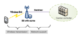
(a) A single-cell scenario.

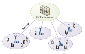
(b) A multi-cell scenario.

Fig. 1: The architecture of a backhaul-limited caching network. BSs are connected to the central controller through separate low-capacity backhaul links. Caches can be allocated to BSs as a supplement to the backhaul.

II-A File Request and Caching Model

The file library has $F$ files, which are assumed to be of the same length $L$ (bits). Note that the same analysis can be applied to the case of unequal file sizes, since files can be divided into chunks of equal length. We do not consider coded caching, and every file is stored as an entire piece. The popularity of file $f,\forall f\in\left\{1,\dots,F\right\}$, can be characterized by a probability mass function $p\left(f\right)$, which can be predicted based on collected data [15, 16], and thus can be regarded as known a priori. Without loss of generality, the files are sorted in the descending order of popularity, i.e., $p\left(1\right)\geq p\left(2\right)\geq\cdots\geq p\left(F\right)$. Mobile users are assumed to make independent requests according to $p\left(f\right)$. Since cooperative caching is beyond the scope of our discussion here, the optimal caching strategy for each BS is to cache the most popular files, and hence the cache hit ratio of cell $j$ can be calculated as

$$h_{j}=\sum_{f=1}^{s_{j}}p\left(f\right),$$ (1)

where $s_{j}\triangleq\left\lfloor\left.c_{S,j}\right/L\right\rfloor$ is defined as the normalized cache size of BS $j$.

II-B File Delivery Model

The delivery of a file depends on two parts: the wireless transmission and the network support (consisting of backhaul transport and cache storage), which will be discussed in detail in this subsection.

We assume no interference among users; e.g., they can be served by different subcarriers with orthogonal frequency-division multiple access (OFDMA). The wireless downlink rate of a user depends on its signal-to-noise ratio (SNR). For simplicity, channel gains are assumed to have the same distribution, and hence it is sufficient to concentrate on one user to study the performance of interest. In cell $j$, with available bandwidth $B_{0}$, the wireless downlink rate of a user is

$$r_{j}=\frac{B_{0}}{U_{j}}\log_{2}\left(1+\frac{P_{t}g_{j}x_{j}^{-\alpha}}{\frac{B_{0}}{U_{j}}\sigma^{2}}\right),$$ (2)

where $P_{t}$ is the BS transmit power, $\sigma^{2}$ denotes the constant additive noise power, $g_{j}$ is the exponentially distributed channel power with unit mean, $\alpha$ is the path-loss exponent, and $x_{j}$ denotes the distance between the target user and the local BS $j$. To avoid interruptions during the playback of the file and guarantee the quality of experience (QoE) of users, the downlink rate $r_{j}$ cannot be lower than the playback rate $r_{0}$. If $r_{j}\geq r_{0}$, the actual rate dedicated to the user will be $r_{0}$ (here we assume fixed rate transmission).

A successful file delivery occurs when both the wireless transmission and the network support meet the requirements. Define the USP of a user in cell $j$ as $P_{j}^{U}$, which is the probability of the user successfully obtaining its requested file. Then, we can compute the success probability by

$$P_{j}^{U}=P_{j}^{W}\cdot P_{j}^{N},$$ (3)

where $P_{j}^{W}$ and $P_{j}^{N}$ stand for the success probability of wireless transmission and network support, respectively. When the downlink rate reaches the required rate $r_{0}$ (bits/sec/Hz), user $k$ will enjoy a successful wireless transmission, and thus we have

$$P_{j}^{W}=\mathbb{P}\left[r_{\left(j\right)_{k}}\geq r_{0}\right].$$ (4)

As for the network support, if the user’s requested file is already stored in the local cache, the user is considered to be successfully supported by the network. Otherwise, the requested file needs to be delivered via the backhaul first. However, the backhaul capacity is limited and usually not all the users demanding backhaul delivery can be supported simultaneously. To be specific, in cell $j$, the largest number of users that can be supported at the same time by the backhaul is given by $\left\lfloor\left.c_{B,j}\right/r_{0}\right\rfloor$. After a successful backhaul delivery, the requested file can be transmitted to the user from BS $j$. Therefore, the network support success probability is given by

$$P_{j}^{N}=h_{j}+\left(1-h_{j}\right)\cdot P_{j}^{B},$$ (5)

where $P_{j}^{B}$ is the probability that the backhaul is available to a user in cell $j$. We define $B_{j}\triangleq\left\lfloor\left.c_{B,j}\right/r_{0}\right\rfloor$ as the normalized backhaul capacity of BS $j$.

III Optimal Cache Size Allocation

In this section, we will first introduce some auxiliary results, then give analysis based on a single-cell scenario, and finally investigate the cache size allocation problem in the multi-cell scenario, for which the optimal solution will be proposed. In addition, we will analyze how the optimal allocation scheme is affected by various system factors, and provide insights for the cache deployment.

III-A Auxiliary Results

In our model, the system performance mainly depends on three factors, namely, wireless transmission, backhaul delivery and cache hits, which will critically affect the cache size allocation. We begin with some auxiliary results for these factors, which will be frequently used in the remainder of the paper.

III-A1 Success Probability of Wireless Transmission

We assume users are uniformly distributed in the cell, and therefore the average success probability is given by the following lemma.

Lemma 1.

In the downlink cellular network model, the success probability of wireless transmission for a user in cell $j$ is

$$P_{j}^{W}=\frac{2}{R_{j}^{2}}\int_{0}^{R_{j}}\exp\left(-\frac{B_{0}\sigma^{2}x^{\alpha}\left(2^{\frac{r_{0}U_{j}}{B_{0}}}-1\right)}{P_{t}U_{j}}\right)x\mathrm{d}x.$$ (6)

Proof:

According to the assumption, the probability density function $f_{X_{j}}(x)$ of the distance $x_{j}$ between a typical user and its serving BS $j$ is $f_{X_{j}}(x)=\frac{2x}{R_{j}^{2}}.$ From (2), the outage probability of a user in cell $j$ can be given as

$$\mathbb{P}\left[r_{j}<r_{0}\right]=\int_{0}^{R_{j}}\mathbb{P}\left[\left.r_{j}<r_{0}\right|x_{j}=x\right]f_{X_{j}}\left(x\right)\textrm{d}x$$

$$=-\frac{2}{R_{j}^{2}}\int_{0}^{R_{j}}\exp\left(-\frac{B_{0}\sigma^{2}x^{\alpha}\left(2^{\frac{r_{0}U_{j}}{B_{0}}}-1\right)}{P_{t}U_{j}}\right)x\textrm{d}x+1.$$ (7)

Since $P_{j}^{W}=1-\mathbb{P}\left[r_{j}<r_{0}\right]$, we can obtain (6). ∎

III-A2 Success Probability of Backhaul Delivery

Denote the number of users who are requiring backhaul delivery in cell $j$ as $U_{j}$. For backhaul delivery, it is assumed that if $U_{j}\leq B_{j}$, all the users can be successfully supported, while if $U_{j}>B_{j}$, $B_{j}$ users will be randomly picked and get successful delivery. So the overall success probability of backhaul delivery is given by the following lemma.

Lemma 2.

If all the users within a cell have an equal chance to be served by the backhaul, the support probability of backhaul delivery for a user in cell $j$ is

$$P_{j}^{B}=\sum_{m=0}^{U_{j}-1}\binom{U_{j}-1}{m}h_{j}^{U_{j}-1-m}\left(1-h_{j}\right)^{m}\cdot\min\left\{1,\frac{B_{j}}{m+1}\right\}.$$ (8)

Proof:

Assume that in addition to the target user, there are another $m$ users requiring backhaul service, $m\in\left\{0,1,\dots,U_{j}-1\right\}$. When $m\leq B_{j}-1$, the target user can always be scheduled to use the backhaul. When $m\geq B_{j}$, the user will get the chance to use backhaul at a probability of $\frac{B_{j}}{m+1}$. Therefore, the support probability of backhaul delivery for a user in cell $j$ can be written as

$$\hskip 15.00002ptP_{j}^{B}=\sum_{m=0}^{B_{j}-1}\binom{U_{j}-1}{m}h_{j}^{U_{j}-1-m}\left(1-h_{j}\right)^{m}$$

$$\hskip 15.00002pt\hskip 25.00003pt+\sum_{m=B_{j}}^{U_{j}-1}\binom{U_{j}-1}{m}h_{j}^{U_{j}-1-m}\left(1-h_{j}\right)^{m}\cdot\frac{B_{j}}{m+1}.$$ (9)

As a result, (8) can be obtained. ∎

III-A3 Cache Hit Ratio

In this paper, we adopt Zipf distribution, an empirical model widely used in related works [5, 6], to model the content popularity. The Zipf distribution states that the popularity $p\left(f\right)$ of file $f$ is inversely proportional to its rank, which is written as

$$p\left(f\right)=\frac{\frac{1}{f^{\gamma_{p}}}}{\sum_{g=1}^{F}\frac{1}{g^{\gamma_{p}}}},$$ (10)

where $\gamma_{p}$ is the Zipf exponent characterizing the distribution. Then the cache hit ratio of cell $j$ is given by

$$h_{j}=\frac{\sum_{f=1}^{s_{j}}\frac{1}{f^{\gamma_{p}}}}{\sum_{g=1}^{F}\frac{1}{g^{\gamma_{p}}}}.$$ (11)

III-A4 User Success Probability

Substituting (5), (6), (8) and (11) into (3), we can obtain the expression of USP as

$$P_{j}^{U}=P_{j}^{W}\cdot\left(\frac{\sum_{f=1}^{s_{j}}\frac{1}{f^{\gamma_{p}}}}{\sum_{f=1}^{F}\frac{1}{g^{\gamma_{p}}}}+\left(1-\frac{\sum_{f=1}^{s_{j}}\frac{1}{f^{\gamma_{p}}}}{\sum_{f=1}^{F}\frac{1}{g^{\gamma_{p}}}}\right)\cdot P_{j}^{B}\right).$$ (12)

III-B The Single-Cell Scenario

We first focus on a single-cell scenario to simplify the analysis. The subscript $j$ which is used to distinguish cells in the aforementioned formulas can be ignored in this case. When the backhaul is fixed, we are interested in the cache size that is required to be allocated to the local BS in order to reach a USP threshold $\theta_{th}$. Thus the problem is formulated as minimizing the cache size allocated to the local BS:

$$\mathcal{Q}\left(\theta_{th}\right):\textrm{minimize} \hskip 10.00002pts$$

subject to $$\hskip 10.00002ptP^{U}\geq\theta_{th},\forall k\in\left\{1,\dots,U\right\}$$

$$\hskip 10.00002pts\in\mathbb{N}.$$

It can be easily checked that $P^{U}$ is monotonically increasing w.r.t. $s$, so we can adopt a bisection search algorithm to solve problem $\mathcal{Q}$ with a computational complexity of $\mathcal{O}\left(\log_{2}\left(F\right)\right)$. In order to gain some insights into the influence of different parameters on the required cache size, we will further provide a closed-form expression for $P^{U}$ and an approximation solution for problem $\mathcal{Q}$.

To begin with, we use the integral form to approximate the popularity of file $f$ as

$$p\left(f\right)\approx\left.\frac{1}{f^{\gamma_{p}}}\right/\int_{0}^{F}\frac{1}{g^{\gamma_{p}}}\textrm{d}g.$$ (13)

Then the cache hit ratio is also rewritten in the form of an integral:

$$h=\int_{0}^{s}p\left(f\right)\textrm{d}f.$$ (14)

For $\gamma_{p}\neq 1$, we can get

$$h\approx\frac{s^{1-\gamma_{p}}-1}{F^{1-\gamma_{p}}-1}.$$ (15)

The result of (8) is relaxed as

$$P^{N} \leq h+\left(1-h\right)\sum_{m=0}^{U-1}\binom{U-1}{m}h^{U-1-m}\left(1-h\right)^{m}\frac{B}{m+1}$$

$$=h+\frac{B}{U}\left(1-h^{U}\right).$$ (16)

Since a probability cannot be greater than 1, we have

$$P^{N}\leq\min\left(h+\frac{B}{U}\left(1-h^{U}\right),1\right).$$ (17)

Note that when $h+\frac{B}{U}\left(1-h^{U}\right)\geq 1$, $P^{N}$ may become close to 1, which means that the network (including caching and backhaul) is always competent to support users, and the USP only depends on the probability of wireless transmission success, i.e., $P^{U}=P^{W}$. However, actually both caching capacity and backhaul capacity are far from enough for user requirements, i.e., $h+\frac{B}{U}\left(1-h^{U}\right)<1$. In fact, we usually have $0\leq h<1$ and $h^{U}\ll 1$, and thus, an approximation for $P^{U}$ can be obtained as

$$P^{U} =P_{k}^{W}\cdot P^{N}\leq P^{W}\left(h+\frac{B}{U}\left(1-h^{U}\right)\right)\leq P^{W}\left(h+\frac{B}{U}\right),$$

$$\approx P^{W}\left(\frac{s^{1-\gamma_{p}}-1}{F^{1-\gamma_{p}}-1}+\frac{B}{U}\right),\textrm{ for }\mbox{$\gamma_{p}\neq$1}$$ (18)

which is a closed-form expression for $P^{U}$. From formula (15) and (18), a tradeoff between the cache size $s$ and backhaul capacity $B$ can be observed in order to achieve the required value of $P^{U}$. Given the USP threshold $\theta_{th}$, we can get the approximated minimum required cache size as

$$s_{\min}\approx\left[\left(\frac{\theta_{th}}{P^{W}}-\frac{B}{U}\right)\left(F^{1-\gamma_{p}}-1\right)+1\right]^{\frac{1}{1-\gamma_{p}}},\textrm{ for }\mbox{$\gamma_{p}\neq$1},$$ (19)

from which some key insights can be gained as follows:

1) When $\gamma_{p}>1$ and $F\gg 1$, we have $s_{\min}\approx\left(1-\frac{\theta_{th}}{P^{W}}+\frac{B}{U}\right)^{\frac{1}{1-\gamma_{p}}}$. In this case, $s_{\min}$ increases exponentially with $\theta_{th}$ and $U$, and decreases exponentially with $B$ and $P^{W}$. Note that $P^{W}$ increases when the cellular wireless channel becomes favorable and $U$ gets smaller. So a larger $U$ will always result in a larger $s_{\textrm{min}}$. Additionally, in this scenario, $s_{\min}$ has nothing to do with $F$, which is due to the highly concentrated popularity distribution, and caching a small subset of files will be sufficient.

2) When $\gamma_{p}<1$ and $F\gg 1$, $s_{\min}\approx\left(\frac{\theta_{th}}{P^{W}}-\frac{B}{U}\right)^{\frac{1}{1-\gamma_{p}}}F$. In this case, $s_{\min}$ also increases exponentially with $\theta_{th}$ and $U$, and decreases exponentially with $B$ and $P^{W}$. Furthermore, $s_{\min}$ increases linearly with $F$. This is because the caches are assumed to store the most popular files, which is the optimal caching strategy when each user is allowed to access only one BS. Consequently, when files are of a relatively uniform popularity, in order to maintain the cache hit ratio, the cache size has to grow linearly with the file library size.

III-C The Multi-cell Scenario

In the multi-cell scenario, the main objective is to find the optimal allocation under a given cache budget. For simplicity, each cell is assumed to operate on an independent bandwidth, and thus the inter-cell inference is ignored. To achieve fairness among different cells, the problem is formulated as maximizing the minimum USP with a normalized cache budget $C_{0}$, and we can obtain the equivalent epigraph form of the optimization problem as

$$\mathcal{P}^{\prime}:\underset{\left\{s_{j}\right\}}{\textrm{maximize}} \hskip 10.00002pt\rho$$

subject to $$\hskip 10.00002ptP_{j}^{U}\geq\rho,\forall j\in\left\{1,\dots,N_{b}\right\}$$

$$\hskip 10.00002pt\sum_{j=1}^{N_{b}}s_{j}\leq C_{0}$$

$$\hskip 10.00002pt0\leq\rho\leq 1$$

$$\hskip 10.00002pts_{j}\in\mathbb{N},\forall j\in\left\{1,\dots,N_{b}\right\}.$$

For a fixed $\rho$, we first decouple problem $\mathcal{P}^{\prime}$ into subproblems w.r.t. each BS, i.e., a series of problems $\left\{\mathcal{Q}\left(\rho\right)\right\}$ to find the minimum cache size for each BS, which follows the solution for the single-cell case. Then we decide whether the total cache size needed is within our cache budget. Based on this idea, the problem can be solved by a bisection search procedure, as presented in Algorithm 1.

Algorithm 1 Bisection Search Algorithm for Cache Size Allocation in the Multi-cell Scenario

Step 0: Initialize $\rho_{\textrm{low}}=0$, $\rho_{\textrm{up}}=1$, $\rho_{\textrm{mid}}=0$;

Step 1: Repeat

1. Set $\rho_{\textrm{mid}}\leftarrow\frac{\rho_{\textrm{low}}+\rho_{\textrm{up}}}{2}$;

2. Solve $N_{b}$ subproblems $\left\{\mathcal{Q}\left(\rho\right)\right\}$ and obtain the minimum cache size $\left\{s_{j}\right\}$ for each subproblem. If $\sum_{j=1}^{N_{b}}s_{j}\leq C_{0}$, set $\rho_{\textrm{low}}=\rho_{\textrm{mid}}$; otherwise, set $\rho_{\textrm{up}}=\rho_{\textrm{mid}}$;

Step 2: Until $\rho_{\textrm{low}}-\rho_{\textrm{up}}<\epsilon$, obtain $\rho^{*}=\rho_{\textrm{mid}}$ and obtain the optimal cache size allocation scheme $\left\{s_{j}^{*}\right\}_{j=1}^{Nb}$;

End

Our formulation aims at achieving a max-min fairness by the cache size allocation. There are a lot of factors influencing the allocation. Since the cellular model considered in this work is backhaul-limited, we can set all the parameters except the backhaul capacities to be identical for every cell. From Algorithm 1, as well as the analysis of the single-cell scenario, some insights for cache deployment have been determined and are given as follows:

1) When the cache budget is small, the BSs with a lower-capacity backhaul will obtain a larger quota of the cache size in oder to enhance their USP to catch up with the other BSs, and some BSs with high-capacity backhaul links may not be able to get caches.

2) When the cache budget exceeds a certain level, the system performance will be saturated. This is because the cache hit ratio for every cell becomes 1 and so does the network support probability, which means that the cellular network is no longer backhaul-limited.

3) Given a USP threshold, with a smaller $\gamma_{p}$, the cache budget will be higher, and the influence of the total number of files will be more significant, and vice versa.

These observations will be verified via simulations in the next section.

IV Simulation Results

In this section, we will present simulation results to verify the effect of cache size allocation and illustrate the impact of various system parameters. In simulations, we use the cellular network parameters as shown in Table I.

TABLE I: Simulation Parameters

Parameter	Value
Cell radius $R_{j}$	20 m
Path-loss exponent $\alpha$	4
Noise power $\sigma^{2}$	-102 dBm
Transmit bandwidth $B_{0}$	10 MHz
BS transmit power $P_{t}$	1 w
Data rate requirement $r_{0}$	2 Mbps

IV-A Backhaul-Cache Tradeoff

Consider a single cellular network where 15 users make random requests within a file library of 1000 files following the Zipf distribution with $\gamma_{p}=0.56$ (suggested by Gill et al. [15]). Fig. 2 explicitly demonstrates the tradeoff between backhaul capacity and cache size for given success probability requirements. It can be observed that our approximation is close to the optimal result, which shows the accuracy of our approximation in the evaluation. We observe that a higher success probability can be achieved by increasing either the backhaul capacity or the cache size. Also, it is shown that when the backhaul capacity is lower, a backhaul augmentation can reduce the cache size more effectively.

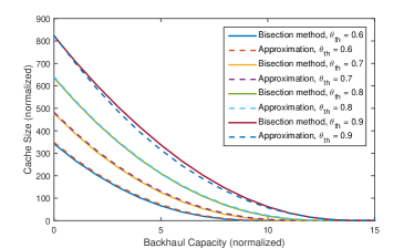
Fig. 2: Cache size versus backhaul capacity.

IV-B Impact of File Popularity Distribution

The file popularity distribution plays a critical role in our system model. We adopt the Zipf distribution, which depends on two parameters, the number of files $F$ (i.e., file library size) and the popularity shape parameter $\gamma_{p}$ (i.e., the Zipf exponent). The effect of these two parameters on the required cache size is plotted in Fig. 3. In Fig. 3(a), we set $\theta_{th}=0.8$, and it can be observed that the cache size increases linearly w.r.t. $F$ when $\gamma_{p}<1$, while the cache size is close to a constant when $\gamma_{p}>1$. The findings are in agreement with the insights indicated in Subsection III-B.

As for the Zipf exponent $\gamma_{p}$, it was estimated as about 0.56 by Gill et al. [15] in a campus setting over three months, and was suggested to be of a higher value of around 1.0 by Cha et al. [16] based on a six-day global trace of a certain category on YouTube. We investigate the effect of $\gamma_{p}$ from 0 to $1.5$. A larger $\gamma_{p}$ stands for a more concentrated popularity distribution. We observe that the required cache size drops dramatically when $\gamma_{p}$ increases, which is because a small cache size is enough to support the system, since a small number of files are responsible for a large number of user requests.

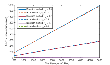
(a) Cache size versus the number of files.

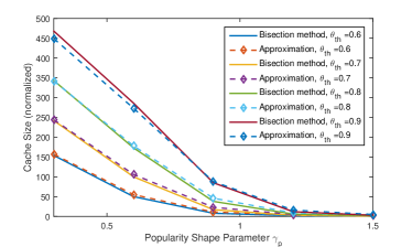
(b) Cache size versus popularity shape parameter.

Fig. 3: The influence of file popularity distribution on cache size.

IV-C Cache Size Allocation for Different Cache Budget

In this subsection, we will demonstrate the cache size allocation scheme under a specific multi-cell scenario consisting of six cells with backhaul capacities of 0, 2, 6, 10, 20 and 28 Mbps, respectively. Except the backhaul conditions, the parameters for each cell are set to be the same as the single-cell case.

In Fig. 4, we plot the performance of the optimal solution and compare it with the uniform allocation of the cache budget. We evaluate the performance for two different kinds of popularity distribution: $\gamma_{p}=1.2$, reflecting a more concentrated popularity distribution, and $\gamma_{p}=0.6$, reflecting a less concentrated one. It is illustrated that with optimization of the cache budget allocation, the performance can be significantly improved, which highlights the importance of cache size allocation. Also, it is noted that the optimal allocation brings more benefits for a smaller $\gamma_{p}.$ To understand this phenomenon, we can image an extreme popularity distribution where all users request the same file. In that case, the uniform allocation will coincide with the optimal allocation. In addition, it is shown that with a larger $\gamma_{p}$, a lower cache budget is needed to reach a given USP, and the change in the file library size will be much more insignificant.

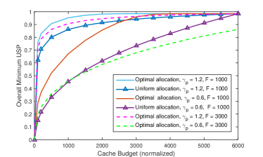
Fig. 4: Overall minimum user success probability versus cache budget.

Fig. 5 shows the details of cache size allocation under different cache budgets with $\gamma_{p}=0.6$ and $F=1000$. When the cache budget is small, the BSs with lower backhaul capacities will have higher priorities to be allocated caches. When the cache budget is large enough, the performance is saturated, and the allocation scheme remains the same since a greater cache budget is no longer useful to improve the system. These behaviors shown in the figure confirm our initial intuition.

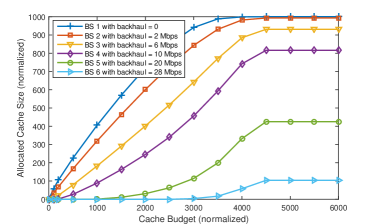
Fig. 5: Cache size allocation scheme under different cache budgets.

V Conclusions

In this paper, we investigated the cache size allocation problem in backhaul limited cellular network, while considering the wireless transmissions and file popularities. In the single-cell scenario, a closed-form expression of the required cache size to achieve a USP threshold was derived to illustrate the impacts of different system parameters. Moreover, the optimum cache size allocation to maximize the overall system performance was studied for the multi-cell scenario. It was shown that the optimal allocation can fully exploit the benefits of caching, and some insights about caching deployment were also discussed.

References

- [1] Cisco Systems Inc., “Cisco visual networking index: Global mobile data traffic forecast update, 2014-2019,” White Paper, Feb. 2015.
- [2] C. Li, J. Zhang, and K. B. Letaief, “Throughput and energy efficiency analysis of small cell networks with multi-antenna base stations,” IEEE Trans. Wireless Commun, vol. 13, no. 5, pp. 2505–2517, May 2014.
- [3] O. Tipmongkolsilp, S. Zaghloul, and A. Jukan, “The evolution of cellular backhaul technologies: Current issues and future trends,” IEEE Commun. Surveys Tuts, vol. 13, no. 1, pp. 97–113, First Quarter 2011.
- [4] X. Ge, H. Cheng, M. Guizani, and T. Han, “5G wireless backhaul networks: challenges and research advances,” IEEE Network, vol. 28, no. 6, pp. 6–11, Nov. 2014.
- [5] E. Bastug, M. Bennis, M. Kountouris, and M. Debbah, “Cache-enabled small cell networks: modeling and tradeoffs,” EURASIP Journal on Wireless Communications and Networking, vol. 2015, no. 1, Feb. 2015.
- [6] K. Shanmugam, N. Golrezaei, A. Dimakis, A. Molisch, and G. Caire, “Femtocaching: Wireless content delivery through distributed caching helpers,” IEEE Trans. Inf. Theory, vol. 59, no. 12, pp. 8402–8413, Dec. 2013.
- [7] X. Peng, J.-C. Shen, J. Zhang, and K. B. Letaief, “Joint data assignment and beamforming for backhaul limited caching networks,” in Proc. IEEE Int. Symp. on Personal Indoor and Mobile Radio Comm. (PIMRC), Washington, DC, Sept. 2014.
- [8] A. Liu and V. Lau, “Exploiting base station caching in MIMO cellular networks: Opportunistic cooperation for video streaming,” IEEE Trans. Signal Process., vol. 63, no. 1, pp. 57–69, Jan. 2015.
- [9] X. Peng, J.-C. Shen, J. Zhang, and K. B. Letaief, “Backhaul-aware caching placement for wireless networks,” in Proc. IEEE Global Telecom. Conf. (GLOBECOM), San Diego, CA, Dec. 2015.
- [10] M. Maddah-Ali and U. Niesen, “Fundamental limits of caching,” IEEE Trans. Inf. Theory, vol. 60, no. 5, pp. 2856–2867, May 2014.
- [11] ——, “Decentralized coded caching attains order-optimal memory-rate tradeoff,” IEEE/ACM Trans. Netw., vol. 23, no. 4, pp. 1029–1040, Aug. 2015.
- [12] D. Leong, A. Dimakis, and T. Ho, “Distributed storage allocation for high reliability,” in Proc. IEEE Int. Conf. Commun. (ICC), Cape Town, South Africa, May 2010.
- [13] Y. Wang, Z. Li, G. Tyson, S. Uhlig, and G. Xie, “Design and evaluation of the optimal cache allocation for content-centric networking,” IEEE Trans. Comput., doi: 10.1109/TC.2015.2409848.
- [14] J. Gu, W. Wang, A. Huang, and H. Shan, “Proactive storage at caching-enable base stations in cellular networks,” in Proc. IEEE Int. Symp. on Personal Indoor and Mobile Radio Commun. (PIMRC), London, UK, Sept. 2013.
- [15] P. Gill, M. Arlitt, Z. Li, and A. Mahanti, “YouTube traffic characterization: A view from the edge,” in Proc. ACM IMC, San Diego, CA, Oct. 2007.
- [16] M. Cha, H. Kwak, P. Rodriguez, Y.-Y. Ahn, and S. Moon, “I tube, you tube, everybody tubes: Analyzing the world’s largest user generated content video system,” in Proc. ACM IMC, San Diego, CA, Oct. 2007.