Flexible Caching in Trie Joins

Abstract

Traditional algorithms for multiway join computation are based on rewriting the order of joins and combining results of intermediate subqueries. Recently, several approaches have been proposed for algorithms that are “worst-case optimal” wherein all relations are scanned simultaneously. An example is Veldhuizen’s Leapfrog Trie Join (LFTJ). An important advantage of LFTJ is its small memory footprint, due to the fact that intermediate results are full tuples that can be dumped immediately. However, since the algorithm does not store intermediate results, recurring joins must be reconstructed from the source relations, resulting in excessive memory traffic. In this paper, we address this problem by incorporating caches into LFTJ. We do so by adopting recent developments on join optimization, tying variable ordering to tree decomposition. While the traditional usage of tree decomposition computes the result for each bag in advance, our proposed approach incorporates caching directly into LFTJ and can dynamically adjust the size of the cache. Consequently, our solution balances memory usage and repeated computation, as confirmed by our experiments over SNAP datasets.

1 Introduction

LeapFrog Trie Join (LFTJ) [24] is a multiway join algorithm introduced by LogicBlox [3] and implemented within. It operates in a manner of variable elimination where there is a linear order over the variables, and query results are generated one by one by incrementally assigning values to each variable in order. Trie indices over the relations guarantee that, throughout execution, one efficiently determines whether the current prefix of assignments cannot be matched against the database (we give a detailed description of LFTJ in Section 2). Veldhuizen [24] has shown that LFTJ is worst-case optimal. This yardstick of efficiency for join algorithms has been introduced by Ngo et al. [17], and it states that for every join query, no algorithm can be asymptotically faster on the space of all instances; in that work they presented the first algorithm that is likewise optimal, later termed NPRR.

More traditional join optimization has been based on decomposing the multiway join into smaller join queries and combining the intermediate results. This approach has roots in Selinger’s pairwise-join enumeration [22], and it includes the application of Yannakakis’s algorithm [25] over a tree decomposition of the query [9, 8]. The advantage of LFTJ over the traditional approach is twofold. First, LFTJ avoids the potential generation of intermediate results that may be substantially larger than the final output size (which is a key property in guaranteeing worst-case optimality). Second, LFTJ is very well suited for in-memory join evaluation, since besides the trie indices it has a close to zero memory consumption. Of course, memory is required for buffering the tuples in the final result, but these are never read and can be safely dumped to higher storage upon need. In the case of an aggregate query (e.g., count the number of tuples in the result), no such requirement arises.

But intermediate results have the advantage that their tuples can be reused, and this is especially substantial in the presence of a significant skew. In our experiments, we have found that LFTJ often loses its advantage to the built-in caching of intermediate results of the traditional approaches, and in particular, LFTJ is often required to apply many repetition of computations. The repeated traverals back and fourth on the trie index generate excessive memory traffic, which has detrimental impact on the performance of database systems [2]. For example, our analysis of the memory load induced by LFTJ found that running a single count 5-cycle query on the SNAP ca-GrQc data set generates over $45\cdot 10^{9}$ memory accesses, whereas running the same query using tree decomposition and Yannakakis’s join generates less than $16\cdot 10^{9}$ accesses. (The implementation of both algorithms is discussed in Section 5.)

Nevertheless, it is not clear how LFTJ can cache results, since every iteration involves a different partial assignment, and variables are interdependent by the query atoms. Our goal in this work is to accelerate LFTJ by incorporating caching in a way that (a) allows for computation reuse, and (b) does not compromise its key advantages. In particular, our goal is to incorporate caching in LFTJ so that it can utilize whatever memory it has as its disposal towards memoization.

To incorporate caching in LFTJ, we build on a recent development in the theory of join optimization, relating worst-case optimality, variable ordering and tree decomposition [11, 10, 23]. Specifically, given a multijoin query, we build a tree decomposition (TD), find an order on the variables such that the order is compatibile with the TD. But unlike existing work, we do not apply the join algorithm on each bag independently, but rather execute LFTJ as originally designed. Yet, throughout the LFTJ execution we may choose to cache partial assignments (based on some decisions that we discuss later) or reuse cached results. The manner by which caching is carried out, as explained in Section 5, is based on the fact that the variable ordering correlates with the TD. In this way, our caching is flexible (i.e., every cached item is optional), and it does not violate the inherent benefits of LFTJ, while dramatically reducing the memory load. Concretely, running the 5-cycle count query described above on the integrated algorithm generates only $1.4\cdot 10^{9}$ memory accesses, which is over 30$\times$ fewer accesses than the original LFTJ algorithm (and over 10$\times$ fewer accesses then tree decomposition with Yannakakis’s join).

But where does one get a TD from? The literature contains a plethora of algorithms with different quality guarantees. The classical graph-theoretic measure refers to the maximal size of a bag, and a generalization to hypergraphs is based on the notion of a hypertree width. The optimal values of those (i.e., realizing the tree width and the hypertree width, respectively) are both NP-hard problems [4, 8], and efficient algorithms exist for special cases and different approximation guarantees [6]. Other notions include decompositions that approximate the minimal fractional hypertree width [14]. Joglekar et al. [10] determine first the variable ordering (in order to guarantee correctness of computing an expression comprising multiple operators), and then find a tree decomposition that complies with this ordering, and has an approximation guarantee against the minimum fractional hypertree width.

In our case, a TD defines a caching scheme, and various factors are likely to determine the effectiveness of this scheme. Importantly, our caches correspond to the adhesions (parent-child intersections), and the adhesion cardinalities are the dimensions of keys of our caches; hence, small adhesions are likely to have higher hit rates. Moreover, caches are more reusable in the presence of skewed data. Hence, we prefer not to use any algorithm that generates a single tree decomposition, but rather to explore a space of such decompositions. We complement existing decomposition approaches with a heuristic algorithm for enumerating TDs, tailored primarily towards small adhesions. Once such a collection of TDs are generated, we generate compatible orders. (In fact, our approach requires a property stronger than compatibility, and we call it strong compatibility.) Given a TD and a compatible order, we can use various techniques for benefit estimation, such as the cost model of Chu et al. [7]. A particular component of our heuristic is an algorithm for enumerating graph separating sets with polynomial delay, without repetitions, and by increasing size.

We experiment on three types of queries: paths, cycles and random graphs, in various sizes. In par with recent studies on join algorithms, we base our experiments on data sets from the SNAP [13] and IMDB workloads. Our experiments compare the performance of LFTJ with and without caching, and Yannakakis’s algorithm over the TD (with each subquery computed separately, as in [23, 21]), as well as other various systems. The results show consistent improvement compared to LFTJ (in orders of magnitude on large queries), as well as general improvement compared to the examined algorithms and systems. As part of our experiments we research several attributes of cached LFTJ, such as running on different TDs and using a different cache sizes.

1.1 Contributions

Our contributions can be summarized as follows.

• We extend LFTJ with caching, without compromising the key benefits. Our caching is executed alongsize LFTJ, and its size can be determined dynamically according to memory availability.

• We devise a heuristic approach to enumerating tree decompositions of a CQ; this approach favors small adhesions, and is based on enumerating graph separating sets by increasing size.

• We present a thorough experimental study that evaluates the effect of caching on LFTJ and compares the results to state-of-the-art join algorithms.

2 Preliminaries

In this section we give preliminary definitions and notation that we use throughout the paper.

2.1 Graphs

We use both directed graphs and undirected graphs in this paper. Let $g$ be a graph. For a subset $U$ of the nodes of $g$, we denote by $g[U]$ the subgraph of $g$ induced by $U$; that is, the subgraph of $g$ that consists of all the nodes of $U$ and all the edges between nodes of $U$. If $V$ is the node set of $g$ and $S$ is a subset of $V$, then $g-S$ denotes the subgraph of $g$ induced by $V\setminus S$. A separating set of $g$ is a set $S$ of nodes such that $g-S$ is disconnected.

2.2 Conjunctive Queries

In this paper we study the evaluation of a Conjunctive Query, or CQ for short, and the problem of counting the number of tuples resulting from this evaluation. As in recent work on worst-case optimal joins [24, 19, 17], we focus here on full CQs, which are CQs without projection. Formally, a full CQ is a sequence $\varphi_{1},\dots,\varphi_{m}$ where each $\varphi_{i}$ is a subgoal of the form $R(t_{1},\dots,t_{k})$ with $R$ being a $k$-ary relation name and each $t_{j}$ being either a constant or a variable. We denote by $\mathsf{vars}(\varphi_{j})$ the set of variables that occur in $\varphi_{j}$, and we denote by $\mathsf{vars}(q)$ the union of the $\mathsf{vars}(\varphi_{j})$ over all atoms $\varphi_{j}$ in $q$ (i.e., the set of all variables appearing in $q$).

Let $q$ be a full CQ. A partial assignment for $q$ is function $\mu$ that maps every variable in $\mathsf{vars}(q)$ to either a constant value or null (denoted $\bot$). If $\mu$ is a partial assignment for $q$, then we denote by $q_{[\mu]}$ the full CQ that is obtained from $q$ by replacing every variable $x$ is with $\mu(x)$, if $\mu(x)\neq\bot$, and leaving $x$ intact if $\mu(x)=\bot$.

The Gaifman graph of a full CQ $q$ is the undirected graph that has $\mathsf{vars}(q)$ as its node set and an edge between every two variables that co-occur in a subgoal of $q$.

2.3 Ordered Tree Decompositions

Let $q=\varphi_{1},\dots,\varphi_{m}$ be a full CQ. A tree decomposition (TD) of $q$ is a pair $\langle t,\chi\rangle$ where $t$ is a tree and $\chi$ is a function that maps every node of $t$ to a subset of $\mathsf{vars}(q)$, called a bag, such that both of the following hold.

• For every subgoal $\varphi_{j}$ there is a node $v$ of $t$ such that $\mathsf{vars}(\varphi_{j})\subseteq\chi(v)$.

• For every variable $x$ in $\mathsf{vars}(q)$, the nodes $v$ of $t$ with $x\in\chi(v)$ induce a connected subtree of $t$.

An ordered TD of a full CQ $q$ is pair $\langle t,\chi\rangle$ defined similarly to a TD, except that $t$ is a rooted and ordered tree. We denote the root of $t$ by $\mathrm{root}(t)$. Let $v$ be a node of $t$. We denote by $t_{|v}$ the subtree of $t$ that is rooted at $v$ and contains all of the descendants of $v$. An adhesion of $t$ is a set of the form $\chi(v)\cap\chi(p)$, where $v$ is a node of $t$ with a parent $p$. The parent adhesion of a non-root node $v$ (or simply the adhesion of $v$) is the set $\chi(p)\cap\chi(v)$ where $p$ is the parent of $v$, and is denoted by $\mathrm{adhesion}(v)$.

Let $q$ be a full CQ, and let $\langle t,\chi\rangle$ be an ordered TD of $q$. The preorder of $t$ is the order $\prec$ over the nodes of $t$ such that for every node $v$ with a child $c$ preceding another child $c^{\prime}$, and nodes $u$ and $u^{\prime}$ in $t_{|c}$ and $t_{|c^{\prime}}$, respectively, we have $v\prec u\prec u^{\prime}$. We denote the preorder of $t$ by $\prec_{\mathsf{pre}}$. For a variable $x$ in $\mathsf{vars}(q)$, the owner bag of $x$, denoted $\mathrm{owner}(x)$, is the minimal node $v$ of $t$, under $\prec_{\mathsf{pre}}$, such that $x\in\chi(v)$. We say that $\langle t,\chi\rangle$ is compatible with an ordering $\langle x_{1},\dots,x_{n}\rangle$ of $\mathsf{vars}(q)$ if for every $x_{i}$ and $x_{j}$, if $\mathrm{owner}(x_{i})$ is a parent of $\mathrm{owner}(x_{j})$ then $i<j$ [10]. We say that $\langle t,\chi\rangle$ is strongly compatible with $\langle x_{1},\dots,x_{n}\rangle$ if for every $x_{i}$ and $x_{j}$, if $\mathrm{owner}(x_{i})\prec_{\mathsf{pre}}\mathrm{owner}(x_{j})$ then $i<j$. Observe that strong compatibility indeed implies compatibility (but not necessarily vice versa).

2.4 Trie Join

Algorithm ${\sf TJCount}(\mbox{$q,\langle x_{1},\dots,x_{n}\rangle,\mathcal{T}$})$

1:  $\mathit{total}:=0$ 2:  for $d=1,\dots,n$ do 3:     $\mu(x_{d}):=\bot$ 4:  ${\sf RJoin}(1)$ 5:  return $\mathit{total}$

Subroutine ${\sf RJoin}(\mbox{$d$})$

1:  if $d=n+1$ then 2:     $\mathit{total}:=\mathit{total}+1$ 3:     return 4:  for all matching values $a$ for $x_{d}$ in $q_{[\mu]}$ and $\mathcal{T}$ do 5:     $\mu(x_{d}):=a$ 6:     ${\sf RJoin}(d+1)$ 7:  $\mu(x_{d}):=\bot$

Figure 1: Count over trie join

We now describe Veldhuizen’s Leapfrog Trie Join (LFTJ) algorithm [24]. Our description is abstract enough to apply to the tributary join of Chu et al. [7]. Let $q=\varphi_{1},\dots,\varphi_{m}$ be a full CQ. The execution of LFTJ is based on a predefined ordering $\langle x_{1},\dots,x_{n}\rangle$ of the $\mathsf{vars}(q)$. The correctness and theoretical efficiency of LFTJ are guaranteed on every order of choice, but in practice the order may have a substantial impact on the execution cost [7]. Moreover, in our instantiation of LFTJ we will use orderings with specific properties.

For each subgoal $\varphi_{k}$, LFTJ maintains a trie structure on the corresponding relation $r$, where each level $i$ in the trie corresponds to a variable $x_{j}$ in $\mathsf{vars}(\varphi_{k})$ and holds values that can be matched against $x_{j}$ so that whenever $x_{j}$ is in a level above $x_{j^{\prime}}$ it holds that $j<j^{\prime}$. Moreover, every path from root to leaf corresponds to a unique tuple of $r$ and vice versa. Sibling values in the trie are stored in a sorted manner, and so, LFTJ applies a sequence of sort-merge-joins as follows. Each trie holds an iterator, which is initialized by pointing the root. First, all the subgoals that contain $x_{1}$ advance their iterators in the first level until a matching value $a$ is found (i.e., all iterators point to $a$). The algorithm then proceeds recursively with the full CQ $Q_{x_{1}/a}$, then proceeds to the next matching value, and so on, until no matching values are found. A balanced-tree storage of the sibling collections in the tries guarantees that alignment of the iterators on matching attributes is done efficiently (in an amortized sense), which in turn guarantees that LFTJ is worst-case optimal [17]. See [24] for more details.

In this paper, it suffices to regard LFTJ abstractly as depicted in the algorithm of Figure 1, and refer to it as trie join. The pseudocode does not compute the join, but in fact counts the tuples in the join; the translation into evaluation is straightforward, but we find the presentation more elegant for count. Moreover, we will later experiment with both evaluation and counting of joins. In the algorithm, the assignments $x_{i}/a$ are represented using a global partial assignment $\mu$ that is updated by the subroutine ${\sf RJoin}$ (Recursive Join). Note that in addition to $\mu$, also global is the variable $\mathit{total}$ (which, in the end, stores the resulting count).

3 Caching in Trie Join

We now describe our proposed incorporation of caching in LFTJ. For simplicity, we will focus on the counting query and show how we extend the algorithm ${\sf TJCount}$ of Figure 1.

3.1 Intuition

The general idea is the following. Given the full CQ $q$, we first construct an ordered TD $\langle t,\chi\rangle$ of $q$. Let $v$ be a node of $t$, let $\alpha$ be $\mathrm{adhesion}(v)$, and let $X$ be the set of all the variables $x$ such that $\mathrm{owner}(x)$ is in the subtree $t_{|v|}$. Then in the result of evaluating $q$ we have the multivalued dependency $\alpha\rightarrow\!\!\!\!\rightarrow X$. Therefore, for every assignment $\mu$ to $\alpha$ we can cache the assignments to $X$ (or their number in the case of counting) and reuse them on the next time $\mu$ is encountered.

One way of obtaining the above caching is by computing the join for every bag using the trie join, and then join the intermediate results using an algorithm for acyclic joins such as that of Yannakakis [25], as done in DunceCap [21, 23]. However, we wish to control the memory consumption of our algorithm and avoid computing full intermediate queries. So, the idea is to run the trie join ordinarily, but then cache results as the algorithm runs, conditioned on a choice of whether or not to cache using some utilization function that estimates the value of caching. For this to work, the ordered TD $\langle t,\chi\rangle$ needs to be strongly compatible with $\langle x_{1},\dots,x_{n}\rangle$, as defined in Section 2.3.

3.2 Algorithm

Our algorithm is depicted in Figure 2. Again, the algorithm is described for the counting problem. The algorithm is an extension of the algorithm of Figure 1 in the sense that when no caching takes place, the two algorithms coincide.

The algorithm, named ${\sf CachedTJCount}$, takes as input a full CQ $q$, an ordered TD $\langle t,\chi\rangle$ for $q$, a variable ordering $\langle x_{1},\dots,x_{n}\rangle$ for $q$, and a database $D$. The algorithm returns the count $|q(D)|$.

The algorithm uses several global variables that are shared across procedure calls.

• As in ${\sf TJCount}$, the global variable $\mathit{total}$ counts the joined tuples and $\mu$ stores the current partial assignment.

• The counter $\mathit{intrmd}(v)$, where $v$ is a node of $t$, stores an intermediate count of the assignments to the variables owned by the nodes in $t_{|v}$, given the assignment to $\mathrm{adhesion}(v)$ in the current iteration. More precisely, let $i$ be the maximal number such that $x_{i}$ is in the adhesion of $x_{i}$, and consider a partial assignment $\mu$ that is nonnull on precisely $x_{1},\dots,x_{i}$. Then in an iteration where $\mu$ is constructed, $\mathit{intrmd}(v)$ will eventually hold the number of assignments $\mu^{\prime}$ for the variables owned by the nodes in $t_{|v}$, such that some full assignment $\hat{\mu}$ for $q$ is consistent with $\mu$. Observe that this number is the same for assignments $\mu$ that agree on the adhesion of $v$. The counter $\mathit{intrmd}(v)$ has the correct value once we are done with the variables owned by $v$.

• $\mathit{cache}$ stores cached values $\mathit{cache}[\alpha,\mu^{\prime}]$ for adhesions $\alpha$ and assignments $\mu^{\prime}$ for $\alpha$. This value is obtained from $\mathit{intrmd}(v)$ once the computation of $\mathit{intrmd}(v)$ is done.

The algorithm ${\sf CachedTJCount}$ simply initializes the global variables and call the subrouting ${\sf RCachedJoin}$, which is the caching version of ${\sf RJoin}$. Next, we explain this subrouting. The input takes not only the variable number $d$, but also a factor $f$ that aggregates cached intermediate counts.

The first part of the algorithm, lines 1–3, tests whether we are done with the variable scan, and if so, adds $f$ to the total count. Now assume that $d\leq n$, and the currently iterated variable is $x_{d}$. Let $v$ be $\mathrm{owner}(x_{d})$ and $\alpha$ be $\mathrm{adhesion}(v)$. In lines 6–12 we handle the case where we have just entered $v$ from a different node of $t$. This is determined by testing whether $d>1$ and the previous variables, $x_{d-1}$, has a different owner (in which case $\mathrm{owner}(x_{d-1})\prec_{\mathsf{pre}}v$ must hold). In that case, the adhesion of $v$ is already assigned values in $\mu$ (since our TD is strongly compatible with the variable ordering), and we check whether we already have a cached result for this assignment. If so, then this cached result is stored in $\mathit{cache}[\alpha,\mu_{|\alpha}]$, where $\mu_{|\alpha}$ is the restriction of $\mu$ to $\alpha$. Hence, if $\mathit{cache}[\alpha,\mu_{|\alpha}]$ is defined, we skip to the next variable outside the subtree $t_{|v}$ with the factor multiplied by $\mathit{cache}[\alpha,\mu_{|\alpha}]$. This skipping is where strong compatibility is required, since it ensures that the nodes owned by $t_{|v}$ constitute a consecutive interval in ${1,\dots,n}$. We then set $\mathit{intrmd}(v)$ to the cached number and return.

Lines 13–18 are executed in the case where we have not entered a new node of $t$ or we so did but did not get a cache hit. In this case, we continue as in ${\sf RJoin}$. In the case where $x_{d}$ is the last variable owned by $v$ (i.e., $d=n$ or $v$ is not the owner of the next variables $x_{d+1}$), we update the intermediate count by adding the product of the intermediate results of the children of $v$. (Note that this product is $1$ when $v$ is a leaf.)

Finally, lines 20–22 consider again the case where we have entered a new node of $v$ from a previous node. At this point, we are about to go back to the previous node, and so, we check whether we should cache for $\alpha$ and $\mu_{\alpha}$. We will consider this choice later, and for now treat it as a decision obtained from a black box. If we indeed choose to cache, then the cached result $\mathit{cache}[\alpha,\mu_{|\alpha}]$ is set to $\mathit{intrmd}(v)$. (This explains why we need to maintain $\mathit{intrmd}(v)$ to begin with.) Next, we give an example of the execution.

Algorithm ${\sf CachedTJCount}(\mbox{$q,\langle t,\chi\rangle,\langle x_{1},\dots,x_{n}\rangle,D$})$

1:  $\mathit{total}:=0$ 2:  for $d=1,\dots,n$ do 3:     $\mu(x_{d}):=\bot$ 4:  for all nodes $v$ of $t$ do 5:     $\mathit{intrmd}(v):=0$ 6:  $\mathit{cache}=\emptyset$ 7:  ${\sf RCachedJoin}(1,1)$ 8:  return $\mathit{total}$

Subroutine ${\sf RCachedJoin}(\mbox{$d,f$})$

1:  if $d=n+1$ then 2:     $\mathit{total}:=\mathit{total}+f$ 3:     return 4:  $v:=\mathrm{owner}(x_{d})$ 5:  $\alpha:=\mathrm{adhesion}(v)$ 6:  if $v\neq\mathrm{owner}(x_{d-1})$ then 7:     $\mathit{intrmd}(v):=0$ 8:     if $\mathit{cache}[\alpha,\mu_{|\alpha}]$ is defined then 9:        let $l$ be the maximum such that $\mathrm{owner}{x_{l}}$ is in $t_{|v}$ 10:        ${\sf RCachedJoin}(l+1,f\cdot\mathit{cache}[\alpha,\mu_{|\alpha}])$ 11:        $\mathit{intrmd}(v):=\mathit{cache}[\alpha,\mu_{|\alpha}]$ 12:        return 13:  for all matching values $a$ for $x_{d}$ in $q_{[\mu]}$ over $D$ do 14:     $\mu(x_{d}):=a$ 15:     ${\sf RCachedJoin}(d+1,f)$ 16:     if $d=n$ or $v\neq\mathrm{owner}(x_{d+1})$ then 17:        let $c_{1},\dots,c_{k}$ be the children of $v$ in $t$ 18:        $\mathit{intrmd}(v):=\mathit{intrmd}(v)+\prod_{i=1}^{k}\mathit{intrmd}(c_{i})$ 19:  $\mu(x_{d}):=\bot$ 20:  if $d>1$ and $v\neq\mathrm{owner}(x_{d-1})$ then 21:     if $(\alpha,\mu_{|\alpha})$ should be cached then 22:        $\mathit{cache}[\alpha,\mu_{|\alpha}]:=\mathit{intrmd}(v)$

Figure 2: Cached count over trie join

Figure 3: Example of a CQ (left) and its tree decomposition (right)

Example 3.1.

The graph on the left side of Figure 3 denotes a query $q$ where every edge corresponds to an atom over a binary relation $R$ with the adjacent variables (that is, $R(x_{1},x_{2})$, $R(x_{2},x_{3})$, $R(x_{2},x_{4})$ and so on). The right side depicts a tree decomposition $\langle t,\chi\rangle$ of $q$. The bags are denoted by the ellipses and adhesions are written in the grey boxes. The tree is directed top down and ordered left to right. Observe that $\langle t,\chi\rangle$ is strongly compatible with $\langle x_{1},\dots,x_{n}\rangle$, which is our order of choice in this example. Finally, our example database $D$ consists of four facts:

$$R(1,1)\quad R(1,2)\quad R(2,1)\quad R(2,2)$$

We now describe a step in ${\sf RCachedJoin}$. As said earlier, this procedure generalizes ${\sf RJoin}$ of Figure 1. We will illustrate the difference between the two.

The first time the procedure reaches an index that changes the owner is for $d=3$, when it moves from the top bag to its child. Denote this child node by $v$. In an iteration with $d=3$, we have $\mathrm{owner}(x_{3})$ is $v$, and the adhesion $\alpha$ is $\{x_{2}\}$. Suppose that $\mu_{|\alpha}(x_{2})=1$. The algorithm then reaches line 8 and tests whether $\mathit{cache}[\{x_{2}\},\mu_{|\alpha}]$ is defined (line 6). On the first variable scan, this test is false, and so, the algorithm will go to line 13. As in ${\sf RJoin}$, the algorithm finds assignments to $x_{3}$ and makes recursive calls. Since $x_{3}$ is not the last node owned by $v$, the test of line 16 is false. Next, the algorithm reaches line 20. If it chooses to cache (for $\alpha$ and $\mu_{|\alpha})$, then $\mathit{intrmd}(v)$ is cached as $\mathit{cache}[\{x_{2}\},\mu_{|\alpha}]$. The value $\mathit{intrmd}(v)$ should be $16$ at this point, since there are $16$ assignments to $x_{3},\dots,x_{6}$ (which are the variables owned by the nodes in the subtree rooted at $v$) that are consistent with $x_{3}$. The value $\mathit{intrmd}(v)$ is determined in the recursive calls of line 15.

The call with the above $\mu$ and $d=3$ later occurs again, and suppose that then $\mathit{cache}[\{x_{2}\},\mu_{|\alpha}]$ is defined. Then the test of line 8 is true, and the algorithm skips to the next index after the last in its subtree, namely $d=7$, with the factor $f$ multiplied by $16$ (which is the value in the cache). In this case, $d=7$, and so, $f$ is added to the total count.

To understand how the intermediate results are calculated, we now consider a call with $d=4$. In this case, $x_{4}$ is the last variable with the owner $v=\mathrm{owner}(x_{4})$. Therefore, the test of line 16 is true. Let $u_{l}$ and $u_{r}$ be the left and right leaves of $t$, respectively. For each match for $x_{4}$, the algorithm adds to $\mathit{intrmd}(v)$ the product $\mathit{intrmd}(u_{l})\cdot\mathit{intrmd}(u_{r})$. The reader can verify that in our example, this produce is always $2\cdot 2=4$. This addition will take place on four assignments for $x_{3}$ and $x_{4}$, and so, $\mathit{intrmd}(v)$ will eventually take the value $4\cdot 4=16$.

3.3 Correctness

The following theorem states the correctness of our algorithm. The proof has two steps. In the first step we prove, by induction on time, that whenever we complete with a node $v$, the number $\mathit{intrmd}(v)$ is correct, that is, it stores the number of intermediate results for the subtree $t_{|v|}$ given the assignment for $\mathrm{adhesion}(v)$. In the second step we prove that every unit added to $\mathit{total}$ accounts for a unique tuple in $q(D)$ and vice versa.

Theorem 3.1.

Let $q$ be a full CQ, $\langle t,\chi\rangle$ a tree decomposition for $q$, and $\langle x_{1},\dots,x_{n}\rangle$ an ordering of $\mathsf{vars}(Q)$ such that $\langle t,\chi\rangle$ is strongly compatible with $\prec_{\mathsf{pre}}$. The algorithm ${\sf CachedTJCount}(q,\langle t,\chi\rangle,\langle x_{1},\dots,x_{n}\rangle,D)$ returns $|q(D)|$.

3.4 Discussion

We now discuss some additional aspects of the algorithm. The decision of line 21 of whether or not to cache may entail arbitrary arguments. In our implementation we adopt a fairly naive approach: we cache only if each assignment has a support (i.e., number of occurrences) larger than a threshold. As we show in Section 5, this already gives us a great benefit; in future work we plan to investigate caching policies in depth. Also, note that the algorithm allows for arbitrary replacements or deletions from the cache.

${\sf CachedTJCount}$ has been described for the task of counting, which is simpler than actually evaluating $q(D)$. Nevertheless, the counting variant of the algorithm entails all of the important aspects, and evaluation would mainly differ in additional details. We discuss those now. First, in evaluation $\mathit{intrmd}(v)$ will contain (representations of) tuple sets. We maintain $\mathit{intrmd}(v)$ only it is actually needed, which means that we decide to cache for either $v$ or an ancestor of $v$. Second, instead of forwardning $f$ in the recursive calls of lines 10 and 15, we forward a sequence of pointers to the intermediate results. Effectively, this means that in the result (which is currently $\mathit{total}$) will constitute a factorized representation [5, 20] that may be decomposed upon need (as we do in the comparisons of our experimental evaluations). Similarly, the product of line 18 is replaced with a factorized representation.

4 Enumerating Decompositions

An important factor in the effectiveness of the caches in the algorithm ${\sf CachedTJCount}$ is their dimensionality, which is determined by the size of the adhesions. Small adhesions imply that are caches have a low dimension, and hence, the chance of a cache hit (i.e., the assignment for the variables in the adhesion has occurred in the past) is higher. There are, however, additional criteria one may wish to apply in the choice of a TD towards beneficial caching. For example, we would like to use adhesions such that their corresponding subqueries have high skews in the data, and then caching a small number of intermediate results can save a lot of repeated computation. Moreover, we would like to have a TD that is strongly compatible with an order that is estimated as good to begin with. Finally, we would like to get decompositions with a large number of bags, so that we can manipulate many caches. Therefore, instead of applying an algorithm that selects a single TD (aiming at optimizing some specific cost function), we take the approach of generating multiple TDs, estimating a cost on each, and selecting the one with the best estimate. In this section, we describe a heuristic algorithm that we use for enumerating a set of “good” TDs where goodness is tailored towards small adhesions. We are not aware of any nontrivial algorithm for enumerating TDs, except for special cases (e.g., chordal graphs [15]) that do not apply here.

4.1 Generic Decomposition

We adopt a simple method for generating tree decompositions. The importance of this method is in the ability to plug to it an algorithm for enumerating graph separating sets, as we explain in the next section. More particularly, the algorithm calls a method for solving the side-constrained graph separation problem, or just the constrained separation problem for short, which is defined as follows. The input consists of an undirected graph $g$ and a set $C$ of nodes of $g$. The goal is to find a separating set $S$ of $g$ (that is, a set $S$ of nodes such that $g-S$ is disconnected). In addition, $S$ is required to have the property that at least one connected component in $g-S$ is disjoint from $C$. Hence, $S$ is required to separate $C$ from some nonempty set of nodes. We call $S$ a $C$-constrained separating set. We denote a call for a solver of this problem by ${\sf ConstrainedSep}(g,C)$. In the next section we will discuss an actual solver. For convenience of presentation, we assume that a solver returns the pair $\langle S,U\rangle$, where $S$ is a $C$-constrained separating set and $U$ is the set of the nodes in the connected components $g^{\prime}$ of $g-C$, such that $g^{\prime}$ intersects (i.e., has a nonempty intersection with) $C$. That is, $U$ is obtained from $g-C$ by taking the union of the connected components $g^{\prime}$ that contain at least one element from $C$. If no such $g^{\prime}$ exists, then we define $U$ to be an arbitrary connected component of $g-C$. Observe that $C\subseteq S\cup U$ holds.

Algorithm ${\sf GenericDecompose}(\mbox{$q$})$

1:  $g:=$ the Gaifman graph of $q$ 2:  return RecursiveTD$(g,\emptyset)$

Subroutine ${\sf RecursiveTD}(\mbox{$g,C$})$

1:  $\langle S,U\rangle\leftarrow{\sf ConstrainedSep}(g,C)$ 2:  if $S=\bot$ then 3:     return the singleton decomposition of $g$ 4:  $\langle t_{0},\chi_{0}\rangle:={\sf RecursiveTD}(g[S\cup U],C\cup S)$ 5:  let $V_{1},\dots,V_{k}$ be the connected comps. of $g-(S\cup U)$ 6:  for $i=1,\dots,k$ do 7:     $\langle t_{i},\chi_{i}\rangle:={\sf RecursiveTD}(g[S\cup V_{i}],S)$ 8:  let $t$ be obtained from $t_{0},t_{1},\dots,t_{k}$ by connecting the root of $t_{0}$ to the root of $t_{i}$ for all $i>1$ 9:  $\chi:=\cup_{i=0}^{k}\chi_{i}$ 10:  return $(t,\chi)$

Figure 4: Tree decomposition via adhesion selection

The algorithm, called ${\sf GenericDecompose}(q)$, is depicted in Figure 4. It takes as input a full CQ $q$ and returns an ordered TD of $q$. It first constructs the Gaifman graph $g$ of $q$, and then calls the subroutine ${\sf RecursiveTD}(g,C)$ with $C$ being the empty set of nodes. The subroutine ${\sf RecursiveTD}(g,C)$ takes as input a graph $g$ and a set $C$ of nodes of $g$, and returns an ordered TD of $g$ with the property that the root bag contains all the nodes in $C$. So, the algorithm first calls ${\sf ConstrainedSep}(g,C)$. Let $\langle S,U\rangle$ be the result. It may be the case that the subroutine decides that no (good) $C$-constrained separating set exists, and then the returned $S$ is null (denoted $\bot$). In this case, the algorithm returns the singleton TD that has only the nodes of $g$ as the single bag. This case is handled in lines 1–3.

So now, suppose that the returned $\langle S,U\rangle$ is such that $S$ is a $C$-constrained separating set. Denote by $V_{1},\dots,V_{k}$ the connected components of $g-(S\cup U)$. The algorithm is then applied recursively to construct several ordered TDs:

• An ordered tree decomposition $\langle t_{U},\chi_{U}\rangle$ of $g[S\cup U]$ (i.e., the induced subgraph of $S\cup U$), such that the root contains $C\cup S$ (line 4);

• For $i=1,\dots,k$, an ordered tree decomposition $\langle t_{i},\chi_{i}\rangle$ of $g[S\cup V_{i}]$, such that the root bag contains $S$ (lines 5–7).

Finally, in lines 8–10 the algorithm combines all of the tree decompositions into a single tree decomposition (returned as the result), by connecting the root of each $\langle t_{i},\chi_{i}\rangle$ to $\langle t_{U},\chi_{U}\rangle$ as a child of the root.

The following proposition states the correctness of the algorithm.

Proposition 4.1.

Let $q$ be a full CQ. ${\sf GenericDecompose}(q)$ returns an ordered TD of $q$.

Example 4.2.

We now describe the algorithm on the CQ $q$ depicted in Figure 3 and described in Example 4.2. The Gaifman graph $g$ of $q$ is the same as $q$, so we refer to $q$ as $g$. We first call RecursiveTD$(g,\emptyset)$. So, suppose that the pair constructed in line 1 is $\langle S,U\rangle$ where $S=\{x_{2}\}$ and $U=\{x_{1}\}$. In line 4 we call the algorithm recursively with $g[\{x_{1},x_{2}\}],\{x_{2}\}$. Note that $g[\{x_{1},x_{2}\}]$ is simply an edge, and so it returns as the singletone decomposition. Moreover, here $k=1$ and $V_{1}=\{x_{3},\dots,x_{6}\}$. In line 7 we call the algorithm with $g[S\cup V_{1}]$ and $S=\{x_{2}\}$. Note that $g[S\cup V_{1}]$ is the graph $g$ with $x_{1}$ removed. Let $\mathcal{T}$ be the TD on the right of Figure 3. If the TD returned from the recursive call is $\mathcal{T}$ with the root removed, then $\mathcal{T}$ is the returned TD. In the execution with the input $g[S\cup V_{1}]$ and $S=\{x_{2}\}$, returned values of ${\sf ConstrainedSep}$ can be $(\{x_{2},x_{3},x_{4}\},\{x_{5}\})$, $(\{x_{3},x_{4}\},\{x_{2}\})$, and so on.

We note that, as defined, ${\sf RecursiveTD}$ may return a TD that contains redundancy in the form of a bag that is contained in another. In this case we can eliminate redundancy by eliminating the smaller bag and connecting its children to the larger set.

4.2 Enumerating Constrained Cuts

The algorithm ${\sf GenericDecompose}(q)$ of Figure 4 generates a single ordered TD. We transform it into an enumeration algorithm by replacing line 1 with a procedure that efficiently enumerates $C$-constrained separating sets, and then executing the algorithm on every such a set. A key feature of the enumeration is that it is done by increasing size of the separating sets, and hence, if we stop the enumeration of separating sets after $k$ sets have been generated (to bound the number the generated TDs), it is guaranteed that we have seen the $k$ smallest $C$-constrained separating sets. So, we are left with the task of enumerating the $C$-constrained separating sets by increasing size. For that, we are using a well known technique for ranked enumeration with polynomial delay.

Lawler-Murty’s procedure [16, 12] reduces a general ranked (or sorted) enumeration problem to an optimization problem with simple constraints. Roughly speaking, to apply the procedure to a specific setting, one needs just to design an efficient solution to the constrained optimization problem. Lawler-Murty’s procedure is a generalization of Yen’s algorithm [26] for finding the $k$ shortest simple paths of a graph. Applying the algorithm gives us the reduction described by the following lemma. In this lemma, a “membership constraint” means a constraint of the form “the result contains a node $v$” or “the result excludes a node $v$.”

Lemma 4.3.

Suppose that, given $g$ and $S$, a minimal $S$-constrained separating set under membership constraints can be found in polynomial time. Then the $S$-constrained separating sets can be enumerated by increasing size with polynomial delay.

So, to get our enumeration it suffices to devise an algorithm for finding a minimal $S$-constrained separating set under membership constraints. This can be done by a reduction to an ordinary minimum-edge-cut problem. The proof is omitted, and will be given in the full version of the paper. Consequently, we get the following theorem.

Theorem 4.3.

Given $g$ and $S$, the $S$-constrained separating sets can be enumerated by increasing size with polynomial delay.

4.3 Discussion

In our implementation (described in the next section), we enumerate TDs by bounding the maximal size of the adhesions (separating sets) in the enumeration that replaces line 1 of ${\sf GenericDecompose}$. To select the actual TD, we employ heuristic cost functions that involve the size of the adhesion, the number bags (higher is better), and the tree’s depth (lower is better). Moreover, we produce a variable ordering from each ordered TD (so that the TD is strongly compatible with the ordering) and apply the cost function of Chu et al. [7]. We leave for future work the investigation of optimizing the TD selection.

5 Experimental Study

Our experimental study examines the performance benefits of our caching in LFTJ, which we call here CLFTJ for short. The counting version of CLFTJ is depicted in Figure 2. To demonstrate that its performance is comparable (and often superior) to common high-performance join algorithms, we also compare it to YTD (Yannakakis and Tree Decomposition). The study explores both count aggregation (denoted as count) and query evaluation. The former computes $|q(D)|$ and the latter computes $q(D)$. Finally, we explore the effect of a number of key parameters of CLFTJ.

5.1 Implementations

Our experiments are based on a vanilla implementation of LFTJ [24]. The implementation of CLFTJ extends the vanilla LFTJ by integrating caches, as described in Section 3 and depicted in Figure 2. STL’s unordered_map is used for the caches, which support indices that consist of up to two dimensions (attributes). The selection of a TD is done as described in Section 4. We first consider caches that store every intermediate result, and later study the impact of bounding the cache.

YTD is implemented by combining Yannakakis’s acyclic join algorithm [25] with TD, as described by Gottlob et al. [9]. Each bag uses ${\sf GenericJoin(abbrev.~{}GJ)}$, a worst-case optimal algorithm [18]. Furthermore, the complexity requirement for the indices seekLowerBound is provided by a binary search, which is enabled through the use of cascading vectors for the Trie. We order the attributes in a manner where the Yannnakakis’s join attributes will be higher in the Trie, similarly to DunceCap [21]. We use the query compiler of EmptyHeaded [1] (which applies an algorithm similar to YTD) to generate the TD. For queries with only two bags we use a regular join since, in this case, the Yannakakis reduction stage generates an unnecessary overhead. Moreover, for count queries whose tree decompositions yields more than two bags, we save the relevant result for the matching join attributes (rather than storing full intermediate results). Notably, we have experimented with alternative YTD implementations, but they all proved inferior to the one described above.

5.2 Methodology

5.2.1 Workloads

In par with other join algorithms, our evaluation is based, for the most part, on datasets from the SNAP collection [13]. The datasets consist of wiki-Vote, p2p-Gnutella04, ca-GrQc, ego-Facebook and ego-Twitter. Since the distribution of values in SNAP dataset is highly skewed, we also use IMDB to explore the effect of datasets that are less skewed and whose data skew is not uniform across attributes. To this end, we partition IMDB’s cast_info table into a male_cast and a female_cast tables, each with attributes (person_id and movie_id).

5.2.2 Queries

We experiment using 3 types of queries:

• {3–7}-path: find paths of lengths 3 to 7 for all possible nodes $a$ and $b$. For example, a valid 4-path can comprise $E(a,b),E(b,c),E(c,d)$.

• {3–6}-cycle: find cycles of length 3 to 6 (e.g., a 4-cycle is $E(a,b),E(b,c),E(c,d),E(a,d)$).

• Random graphs: we generate random graphs using the Erdös-Reyni generator. The generator sets the number of nodes to $N$ and uses a probability $P$ to generate an edge between two nodes. The graph is undirected, contains no self edges, and has at most one edge between two nodes. We use only connected graphs with $N=\{5,6\}$ and $P=\{0.4,0.6\}$. Random graph queries are denoted as $N\textsf{-rand}(P)$. For example, $5\textsf{-rand}(0.4)$ is a random graph where $N=5$ and $P=0.4$. For each set of parameters we generate six different graphs.

Note that we do not examine clique queries since they cannot be decomposed and, therefore, CLFTJ will not offer any advantage over LFTJ on this type of a query.

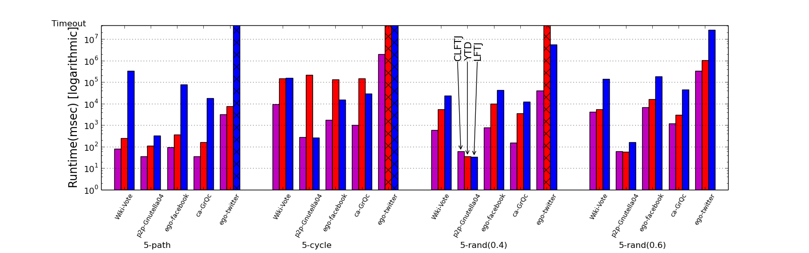
Figure 5: The runtimes observed when executing count queries using the different algorithms. YTD failed to execute 7-rand queries because its requirements exceeded the machines’ memory capacity, and its results are omitted. Bars that represent executions that times out are marked with a crisscross pattern.

5.2.3 Algorithms

The main algorithms we compare against are LFTJ and YTD. In addition to pure algorithms, we also experiment with full systems:

• System 1(SYS1): A DBMS using a worst case-optimal join algorithm as its join engine.

• System 2(SYS2): Another DBMS using a worst case-optimal join algorithm which uses aggressive vector parallelism as its join engine.

• PostgreSQL 9.3.4 (PGSQL): An open source relational DBMS. For optimal results, the optimizer is configured to avoid merge joins and materialization.

Of course, a system has a necessarily overhead that pure algorithms do not have. We make this comparison simply to provide a context for the recorded running times. We further emphasize that our experiments are restricted to a single core, which means that we needed to restrict the above system from utilizing our cores.

We omit other DBMSs and graph engines from our experimental study, as they were already compared to these systems in a previous study [19].

5.2.4 Hardware and System setup

We use Supermicro 2028R-E1CR24N servers as our experimental platform. Each server is configured with two Intel Xeon E5-2630 v3 processors running at 2.4 GHz, 64GB of DDR3 DRAM, and is running a stock Ubuntu 14.0.4 Linux.

5.2.5 Testing Protocol

Each experiment was run three times, and the average runtime is reported. We set an execution timeout of 10 hours. Executions that timed out are highlighted, and their related speedup/slowdown is conservatively computed as if they completed the run at the timeout mark.

5.3 Experimental Results

We experimented with both counting and evaluation for full CQs. We present the results for each type separately.

5.3.1 Count queries

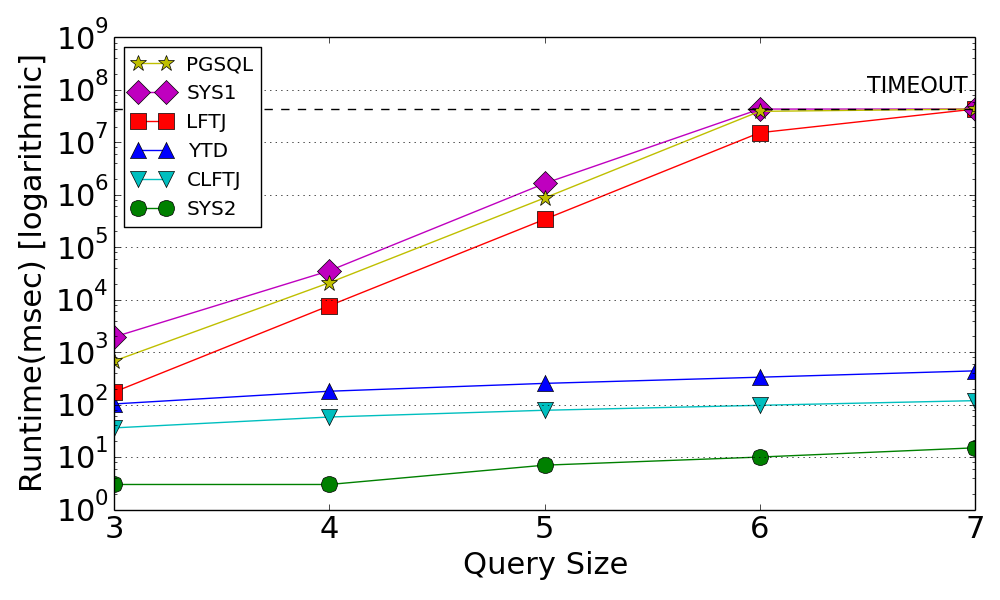
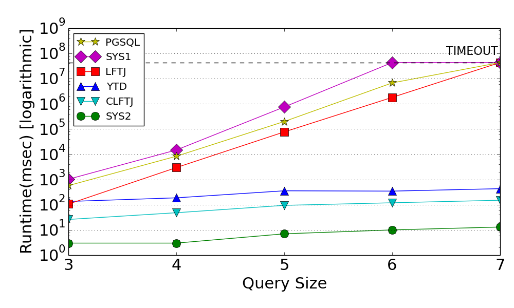
Figure 6: The runtimes observed when executing {3–7}-path count queries on both the clean algorithms and DBMSs. Results shown for wiki-Vote (left) and the ego-Facebook (right) datasets.

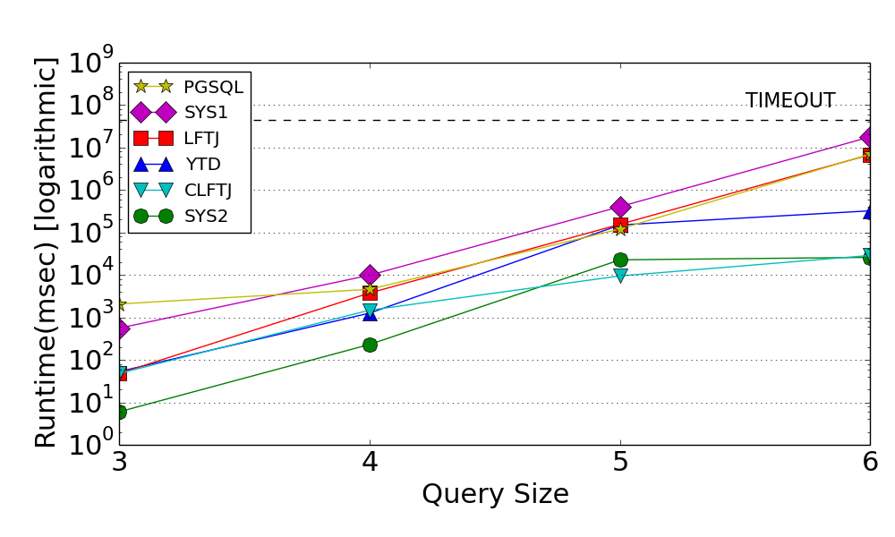
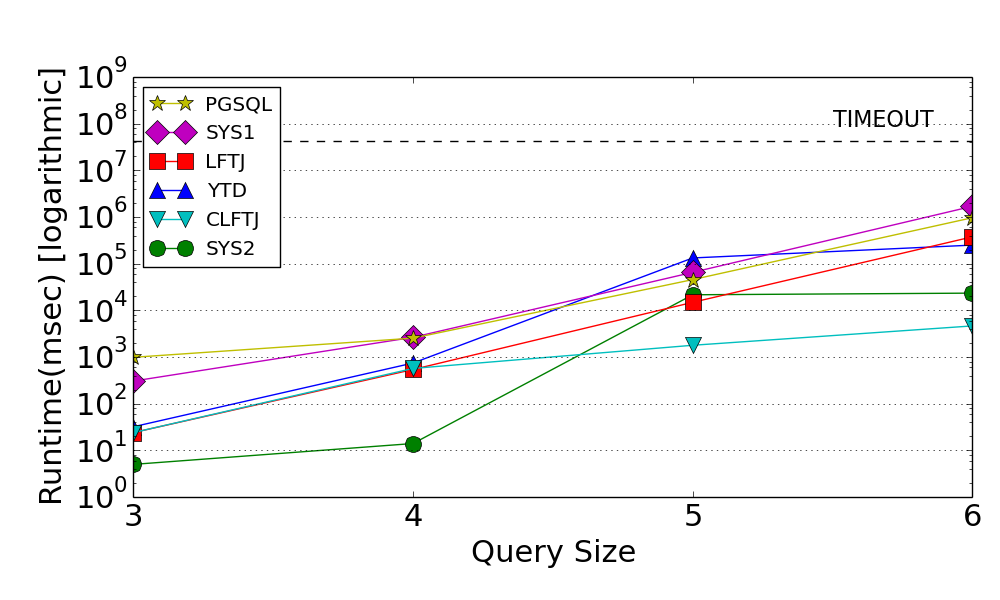
Figure 7: The runtimes observed when executing {3–6}-cycle count queries on both the clean algorithms and DBMSs. Results shown for wiki-Vote (left) and the ego-Facebook (right) datasets.

We first examine the performance of count queries. Figure 5 presents the runtime of 5-path, 5-cycle, and 5-rand queries on different datasets. The figure shows that CLFTJ is faster than the alternatives on 5-path and 5-cycle.

The results demonstrate the effectiveness of CLFTJ when running on datasets that are large and whose value distribution is skewed—two properties that make them highly amenable to caching. For example, the ego-Twitter dataset exhibits these properties and is therefore amenable to caching. When comparing the performance of the different algorithms, we see that CLFTJ is consistently 2–5$\times$ faster than YTD and orders of magnitude faster than LFTJ. On the other extreme, we have the p2p-Gnutella04 dataset that is relatively small and whose value distribution is fairly balanced. For this dataset, the performance benefits of CLFTJ are moderate (for 5-rand queries, both YTD and LFTJ even marginally outperform CLFTJ).

Notably, the results are consistent across different query sizes. Figure 6 presents the runtimes observed when running {3–7}-path queries. (The figure also examines the performance of full systems, which is discussed later in Section 5.3.5 below.) For brevity, we show the results for only two of the datasets. The figure shows that the speedups delivered by CLFTJ over LFTJ even grows with the size of the query. Furthermore, it shows that CLFTJ is even faster than YTD by more than 3$\times$.

Figure 7 examines the performance of CLFTJ for {3–7}-cycle queries (again with systems discussed in Section 5.3.5). Again, the figure shows that CLFTJ outperforms LFTJ and YTD, especially on larger cycle queries. Interestingly, we see little difference in the algorithms’ running times for small, 3-cycle queries. The reason for that is there is no tree decomposition for triangles, and CLFTJ is effectively LFTJ. Similarly, the performance of CLFTJ and YTD is comparable, as YTD uses GJ for {3–4}-cycle queries.

When comparing the benefits of CLFTJ over large cycle queries (Figure 7) and path queries (Figure 6), we see that CLFTJ delivers better speedups for paths. This is attributed to the cache dimension property (the size of adhesions). Therefore, the cache dimension for paths is set to one, and for cycles it is set to two. Notably, a cache whose dimension is one shows as much more effective. Another interesting result in the case of 5-cycle is that YTD performs worse than LFTJ (and underperforms CLFTJ). This is because YTD and GJ favor the opposite attributes order, which dramatically affects its performance.

Finally, Figure 5 presents the running times for random graph queries. The figure presents the results of two representative 5-rand queries. Over all of the $5\textsf{-rand}(0.4)$ and $5\textsf{-rand}(0.6)$ queries, CLFTJ is consistently faster by orders of magnitude than LFTJ on average across datasets. The only exception is the p2p-Gnutella04, which CLFTJ is slightly slower by 1.7$\times$ on two queries and faster by 200$\times$ for the others. Compared to YTD there is a consistent speedup of an $\sim$8$\times$, with exception of one query where YTD is faster by 2$\times$. The results for 6-rand are consistent with 5-rand, with one exception of similar runtime on 6-clique query.

5.3.2 Query Evaluation

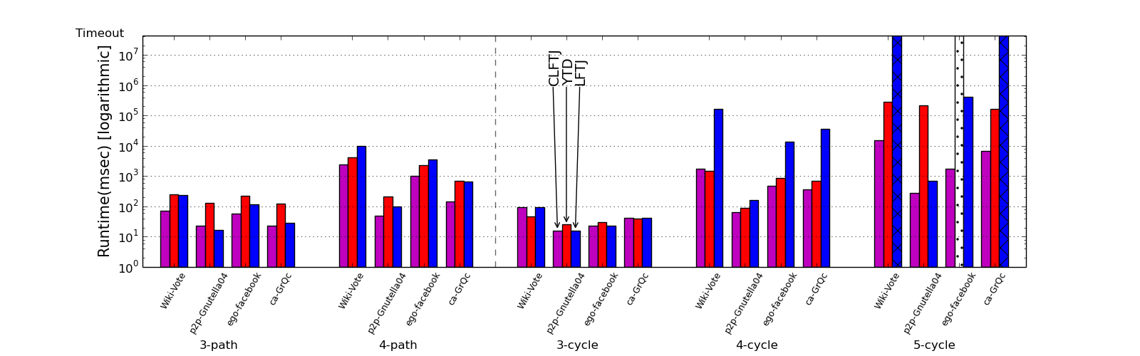
Figure 8: The runtimes of the join algorithms for full query evaluation of path and cycles queries. Queries that failed due to lack of memory are shown as white dotted bars.

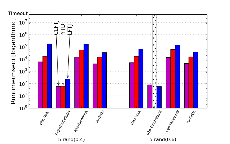
Figure 9: The runtimes of full query evaluation of random graphs. Queries that failed due to lack of memory are shown as white dotted bars.

Query evaluation produces all the tuples in the result of the query (as opposed to counting thereof). Since our experiments measure the total query execution runtime, including the time required to generate the materialized result, the performance benefits of CLFTJ are expected to be less pronounced than for count queries. In contradistinction, the generation of intermediate results during query evaluations may affect the runtime of YTD. Specifically, YTD generates the intermediate results for all bags, even if they will not be used in the final materialized result. In contrast, a key property of LFTJ (and CLFTJ) is that the algorithm generates only intermediate assignment that can be matched along with the entire prefix assignment (according to the variable order). The performance of YTD may thus be affected by the generation of excessive intermediate results.

Importantly, we focus our exploration of query evaluation on computing the materialized result rather then storing it, and ignore queries for which the materialized result does not fit in our machines’ 64GB RAM. For this reason, we only show results for {3–4}-path and {3–5}-cycle queries, and do not discuss the ego-Twitter data set.

The results for running {3–4}-path query evaluations are depicted in Figure 8. The figure shows that, while gains over LFTJ are marginal for the smaller 3-path queries, CLFTJ outperforms LFTJ on the larger 4-path queries by up to 4.6$\times$ (3.5$\times$ on average). The performance gap is attributed to CLFTJ’s caching, which captures frequently used intermediate results. In turn, this eliminates many redundant memory operations executed by LFTJ. The CLFTJ also outperforms YTD by up to 4.6$\times$ (3.2$\times$ on average), since the computation of YTD, which uses Yannakakis joins, becomes memory bound in the final join stages.

Figure 8 also presents the execution time of {3–5}-cycle query evaluations. The figure shows that CLFTJ is faster than LFTJ by 2000$\times$ on average for the larger 5-cycle queries. Interestingly, CLFTJ also proves faster than YTD by up to 800$\times$ (280$\times$ on average) for 5-cycle queries. Similar to path queries, this performance gap is attributed to the excessive number of memory operations issued by the Yannakakis join algorithm in the final stages of the join.

Finally, CLFTJ also delivers performance benefits for random graphs queries. Figure 9 shows the results for representative graphs (which are consistent with the results for the other graphs). Specifically, for $5\textsf{-rand}(0.4)$ queries, CLFTJ outperforms LFTJ by 4–30$\times$. CLFTJ is also consistently 3–4$\times$ faster than YTD, with the exception of p2p-Gnutella04 for which the results are comparable. These trends are also consistent for denser $5\textsf{-rand}(0.6)$ random graphs. Here too, the results demonstrate the effectiveness of CLFTJ, whose runtime is, on average, $\sim$10$\times$ faster than LFTJ and $\sim$4$\times$ than YTD (CLFTJ and LFTJ runtimes are comparable for p2p-Gnutella04).

5.3.3 Dynamic Cache Size

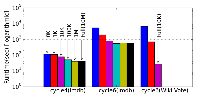
Figure 10: Different cache sizes on {4,6}-cycles count aggregation query over the IMDB dataset and 6-cycle over wiki-Vote dataset

A key benefit of LFTJ is that its memory footprint is proportional to the original dataset and does not depend on any intermediate results. This key property is preserved in CLFTJ through the ability to dynamically bound its cache sizes. Consequently, CLFTJ offers substantial speedups when executing large queries or, alternatively, when running in environments with limited memory resources. Moreover, dynamic cache bounds allow CLFTJ to support multi-tenancy of queries while preserving quality of service.

Figure 10 presents the runtime required to execute a 4-cycle and 6-cycle count aggregation queries (shown in Figure 14) over the IMDB dataset using different overall cache sizes. The figure shows that the speedup provided by CLFTJ is proportional to the overall cache sizes. Moreover, it shows that even small caches provide substantial speedups. For example, caching only 100K intermediate results delivers a 2.5$\times$ speedup on 4-cycle and 7$\times$ speedup on 6-cycle, while caching 1M intermediate results provides a 3$\times$ speedup on 4-cycle and 10$\times$ on 6-cycle. Ultimately, caching all intermediate results using a capacity of 10M results even incurs a small slowdown, due to the sparse use of memory.

Figure 10 presents the same experiment on 6-cycle for the Wiki-Vote dataset. The Wiki-Vote dataset is much smaller and more skewed that can be fully cached with only 10K cache entries. In this case, the optimal 246$\times$ speedup is achieved using a full cache.

We conclude that bounded caches enables CLFTJ to benefit from both worlds. One one hand, it delivers substantial speedups over LFTJ while preserving the bounded memory footprint property. On the other hand, it can execute in settings where traditional join algorithms, which store all intermediate results, either cannot execute or suffer substantial slowdowns due to disk I/O.

5.3.4 Tree Decomposition

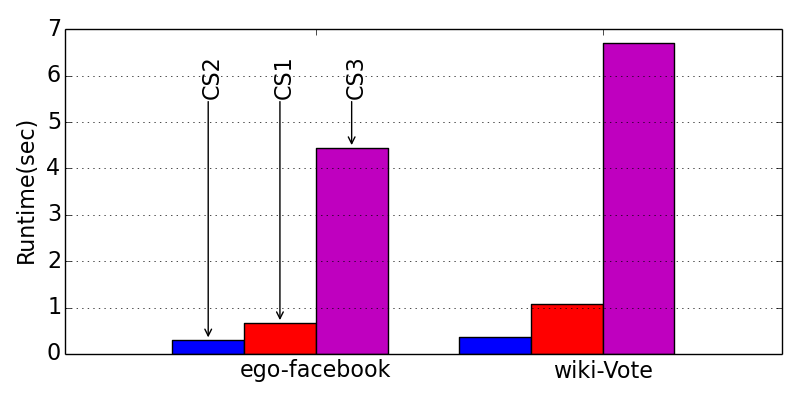
Figure 11: Runtime for the {3,2}-lollipop query (Figure 12) with different cache structures.

Figure 12: $\{3,2\}$-lollipop query and TDs: CS1(left), CS2(middle) and CS3(right)

The next experiment considers the impact of orderings and strongly-compatible TDs on the running time. The results are in Figure 11. The figure presents the runtime of CLFTJ on a {3,2}-lollipop query with different cache structure. Importantly, due to the triangle in the lollipop graph, the treewidth is 2. We compare the CLFTJ runtime on three cache structures that provide the same treewidth: a single 1-dimension cache (CS1), two 1-dimension caches (CS2), and a cache structure with a single 1-dimension and a single 2-dimension caches (CS3). The figure shows that CS1 provides a speedup of 70–80$\times$ over LFTJ, CS2 provides a speedup of 180–190$\times$, and CS3 only provides a speedup of 10$\times$. These results demonstrate that the CLFTJ decomposition should not target (only) small treewidth, but rather its adhesions.

The data skew in cached attributes is another important factor that impacts CLFTJ’s performance, yet common tree decomposition algorithms do not take data properties into account. We demonstrate the effect of data skew on CLFTJ performance using the IMDB dataset, whose different attributes manifest different degrees of data skew.

Figure 14 depicts two TDs, TD1 and TD2, of two queries, 4-cycle and 6-cycle, and Figure 13 presents their respective runtimes. TD1 favors person_id for caching and TD2 favors movie_id for caching. While the decompositions are isomorphic (similar from a graph perspective), we see that their performance vary greatly. The reason for the performance variation is that the person_id attribute exhibits greater data skew than the movie_id. It is therefore more effective to apply caches to the person_id attribute.

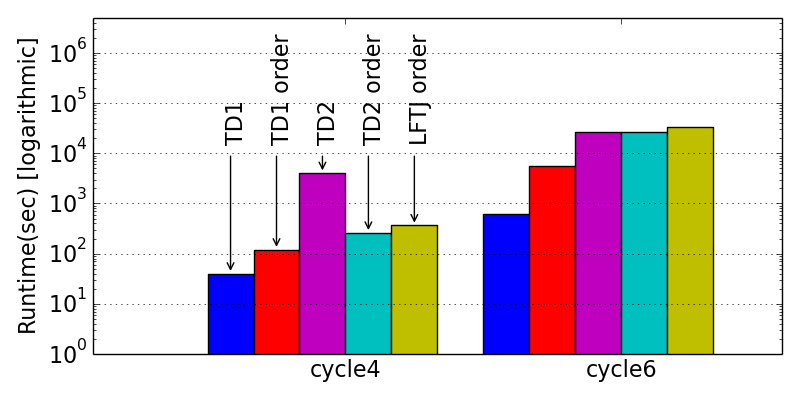
Figure 13: Comparison of CLFTJ with different TDs on 4-cycle and 6-cycle and LFTJ with the imposed decompositions’ attributes order experimented on count aggregation on IMDB dataset

Another interesting result is the performance impact of the order of attributes. For each TD, we selected an ordering such that the TD is strongly compatible with the ordering. Simply using LFTJ with the imposed attribute order offers a 10$\times$ speedup over the original LFTJ order. Notably, a recent study by Chu et al. [7] proposed a method to estimate the cost of attributes order in LFTJ. The method estimates the cost of TD2_order to be $\sim$2$\times$ higher than TD1_order. The runtimes of the different attributes orders is shown in Figure 13. Hence, in these queries the cost function of Chu et al. [7] turns out to be very beneficial as parameter of choosing the TD for caching.

Figure 14: 4-cycle (top) and 6-cycle (bottom) queries on IMDB and TDs: TD1 (left), TD2 (right).

5.3.5 Comparison to Systems

To explore the scaling trends of the pure algorithms, compared to those of the DBMSs, we ran the queries on PGSQL (using pair-wise join), SYS1 and SYS2 (which are based on worst-case optimal join algorithms). For brevity, we show the results for only two datasets: Wiki-Vote and ego-Facebook. Notably, these are consistent with the results obtained for the other SNAP datasets.

Figure 6 shows the results for {3–7}-path count queries. The first thing to note in the figure is that the scaling of vanilla LFTJ and SYS1 are correlated. We attribute the 10$\times$ performance difference between the two to the overheads associated with running a full DBMS vs. a pure algorithm. Importantly, the figure demonstrates that the performance benefit of CLFTJ and YTD over LFTJ increases with the query size at an exponential rate. Moreover, it also shows that even though CLFTJ and YTD have similar scaling trends for path queries, CLFTJ runs almost an order of magnitude faster.

Figure 7 depicts a similar comparison for the queries {3–6}-cycle. Again, the figure shows consistent scaling trends for the vanilla algorithms and the DBMSs that utilize them. A comparison between SYS2 and YTD shows that SYS2 is much faster than YTD. In this case, the DBMS is faster than a pure algorithm since its implementation is massively parallelized using the processor’s wide vector unit. Due to the parallel implementation, SYS2 is much faster than LFTJ on path queries. Nevertheless, the sequential CLFTJ implementation is still comparable to SYS2 for {5–6}-cycles queries (and is even faster on some datasets).

6 Concluding Remarks

We have studied the incorporation of caching in LFTJ by tying an ordered tree decomposition to the variable ordering. The resulting scheme retains the inherent advantages of LFTJ (worst case optimality, low memory footprint), but allows it to accelerate performance based on whatever memory it decides to (dynamically) allocate. Our experimental study shows that the result is consistently faster than LFTJ, by orders of magnitude on large queries, and usually faster than other state of the art join algorithms.

This work gives rise to several directions for future work. These include the exploration of caching strategies, finding decompositions with beneficial caching, extension to general aggregate operators (e.g., based on the work of Joglekar et al. [10] and Khamis et al. [11]), utilizing factorized representations [5, 20], and generalizing beyond joins [24].

References

- [1] C. R. Aberger, A. Nötzli, K. Olukotun, and C. Ré. EmptyHeaded: Boolean algebra based graph processing. CoRR, abs/1503.02368, 2015.
- [2] A. Ailamaki, D. J. DeWitt, M. D. Hill, and D. A. Wood. DBMSs on a modern processor: Where does time go? In Intl. Conf. on Very Large Data Bases (VLDB), pages 266–277, 1999.
- [3] M. Aref, B. ten Cate, T. J. Green, B. Kimelfeld, D. Olteanu, E. Pasalic, T. L. Veldhuizen, and G. Washburn. Design and implementation of the logicblox system. In SIGMOD Conf., pages 1371–1382, 2015.
- [4] S. Arnborg, D. Corneil, and A. Proskurowski. Complexity of finding embeddings in a k-tree. SIAM J. Alg. Disc. Meth., 8(2):277–284, 1987.
- [5] N. Bakibayev, T. Kociský, D. Olteanu, and J. Zavodny. Aggregation and ordering in factorised databases. Proc. of the VLDB Endowment (PVLDB), 6(14):1990–2001, 2013.
- [6] V. Bouchitté, D. Kratsch, H. Müller, and I. Todinca. On treewidth approximations. Discrete Applied Mathematics, 136(2-3):183–196, 2004.
- [7] S. Chu, M. Balazinska, and D. Suciu. From theory to practice: Efficient join query evaluation in a parallel database system. In SIGMOD Conf., pages 63–78, 2015.
- [8] G. Gottlob, M. Grohe, N. Musliu, M. Samer, and F. Scarcello. Hypertree decompositions: Structure, algorithms, and applications. In Intl. Workshop on Graph-Theoretic Concepts in Computer Science (WG), pages 1–15, 2005.
- [9] G. Gottlob, N. Leone, and F. Scarcello. Hypertree decompositions and tractable queries. In Symp. on Principles of Database Systems (PODS), pages 21–32, 1999.
- [10] M. Joglekar, R. Puttagunta, and C. Ré. Aggregations over generalized hypertree decompositions. CoRR, abs/1508.07532, 2015.
- [11] M. A. Khamis, H. Q. Ngo, C. Ré, and A. Rudra. FAQ: questions asked frequently. CoRR, abs/1504.04044, 2015.
- [12] E. L. Lawler. A procedure for computing the best solutions to discrete optimization problems and its application to the shortest path problem. Management Science, 18(7):401–405, 1972.
- [13] J. Leskovec and A. Krevl. SNAP Datasets: Stanford large network dataset collection, 2014.
- [14] D. Marx. Approximating fractional hypertree width. ACM Trans. on Algorithms, 6(2), 2010.
- [15] Y. Matsui, R. Uehara, and T. UNO. Enumeration of perfect sequences of chordal graph. In Intl. Symp. on Algorithms and Computation (ISAAC), 2008.
- [16] K. G. Murty. An algorithm for ranking all the assignments in order of increasing cost. Operations Research, 16(3):682–687, 1968.
- [17] H. Q. Ngo, E. Porat, C. Ré, and A. Rudra. Worst-case optimal join algorithms: [extended abstract]. In Symp. on Principles of Database Systems (PODS), pages 37–48, 2012.
- [18] H. Q. Ngo, C. Re, and A. Rudra. Skew strikes back: New developments in the theory of join algorithms. CoRR, abs/1310.3314, 2013.
- [19] D. T. Nguyen, M. Aref, M. Bravenboer, G. Kollias, H. Q. Ngo, C. Ré, and A. Rudra. Join processing for graph patterns: An old dog with new tricks. In Graph Data-management Experiences & Systems Workshop (GRADES), pages 2:1–2:8, 2015.
- [20] D. Olteanu and J. Závodný. Size bounds for factorised representations of query results. ACM Trans. on Database Systems (TODS), 40(1):2, 2015.
- [21] A. Perelman and C. Ré. DunceCap: Compiling worst-case optimal query plans. In SIGMOD Conf., pages 2075–2076, 2015.
- [22] P. G. Selinger, M. M. Astrahan, D. D. Chamberlin, R. A. Lorie, and T. G. Price. Access path selection in a relational database management system. In SIGMOD Conf., pages 23–34, 1979.
- [23] S. Tu and C. Ré. DunceCap: Query plans using generalized hypertree decompositions. In SIGMOD Conf., pages 2077–2078, 2015.
- [24] T. L. Veldhuizen. Triejoin: A simple, worst-case optimal join algorithm. In Intl. Conf. on Database Theory (ICDT), pages 96–106, 2014.
- [25] M. Yannakakis. Algorithms for acyclic database schemes. In Intl. Conf. on Very Large Data Bases (VLDB), pages 82–94, 1981.
- [26] J. Y. Yen. Finding the shortest loopless paths in a network. Management Science, 17:712–716, 1971.