Problems for the WELS classification of planetary nebulae central stars: Self-consistent nebular modelling of four candidates.

Abstract

We present integral field unit (IFU) spectroscopy and self-consistent photoionisation modelling for a sample of four southern Galactic planetary nebulae (PNe) with supposed weak emission-line (WEL) central stars. The Wide Field Spectrograph (WiFeS) on the ANU 2.3 m telescope has been used to provide IFU spectroscopy for NGC 3211, NGC 5979, My 60, and M 4-2 covering the spectral range of 3400-7000 Å. All objects are high excitation non-Type I PNe, with strong He II emission, strong [Ne V] emission, and weak low-excitation lines. They all appear to be predominantly optically-thin nebulae excited by central stars with $T_{\rm eff}>10^{5}$ K. Three PNe of the sample have central stars which have been previously classified as weak emission-line stars (WELS), and the fourth also shows the characteristic recombination lines of a WELS. However, the spatially-resolved spectroscopy shows that rather than arising in the central star, the C IV and N III recombination line emission is distributed in the nebula, and in some cases concentrated in discrete nebular knots. This may suggest that the WELS classification is spurious, and that, rather, these lines arise from (possibly chemically enriched) pockets of nebular gas. Indeed, from careful background subtraction we were able to identify three of the sample as being hydrogen rich O(H)-Type. We have constructed fully self-consistent photoionization models for each object. This allows us to independently determine the chemical abundances in the nebulae, to provide new model-dependent distance estimates, and to place the central stars on the H-R diagram. All four PNe have similar initial mass ($1.5<M/M_{\odot}<2.0$) and are at a similar evolutionary stage.

1 Introduction

Planetary nebulae represent an advanced stage in the evolution of low and intermediate mass stars as they make the transition between the asymptotic giant branch (AGB) and the white dwarf (WD) stages. The gaseous nebula which appears now as a planetary nebula (PN) is the remnant of the deep convective envelope that surrounded the central core of AGB. This core is now revealed as the central star (CS) of the PN. Thus the PNe provide fundamental data on the mass-loss processes during the AGB stage, the chemical enrichment of the envelope by dredge-up processes, as well as information about the mass, and effective temperature of the remaining stellar core.

Up to now, most studies of the emission line spectra of PNe have been derived from long-slit spectroscopic work. However, an accurate derivation of the physical conditions and chemical abundances in the nebular shell relies upon a knowledge of the integrated spectra. For Galactic PNe, this can only be determined using integral field spectroscopic instruments. This field was pioneered by Monreal-Ibero et al. (2005) and Tsamis et al. (2007), although it is only recently that detailed physical studies using optical integral field data have been undertaken, amongst which we can cite Monteiro et al. (2013) (NGC 3242), Danehkar et al. (2013) (SuWt 2), Danehkar et al. (2014) (Abell 48), Danehkar & Parker (2015) (Hen 3-1333 and Hen 2-113) and Ali et al. (2015b) (PN G342.0-01.7). In this paper, we will analyse integral field data obtained with the WiFeS integral field spectrograph (Dopita et al., 2007; Dopita et al., 2010) to derive plasma diagnostics, chemical composition, and kinematical parameters of the four highly excited nebulae NGC 3211, NGC 5979, My 60, and M 4-2 and to study the properties of the central stars (CSs) of these objects, which from the evidence of their spectra alone, appear to belong to the class of weak emission-line stars (WELS), Tylenda et al. (1993), whose properties are described below.

Reviewing the literature, none of our target objects have been subject to an individual detailed study. However, many of their nebular properties and central star characteristics have been derived and the results are distributed amongst a large number of articles, particularly in the cases of NGC 3211 and NGC 5979. From imaging data, the nebula NGC 3211 was classified as an elliptical PNe (Górny et al., 1999) with an extended halo of radius $\sim$ 3.2 times that of the main nebular shell (Baessgen & Grewing, 1989). The plasma diagnostics and elemental abundances of the object were studied in a few papers (Perinotto, 1991; Milingo et al., 2002). The central star of NGC 3211 has several temperature and luminosity estimates: 135 kK & 2500 L_⊙ (Shaw & Kaler, 1989); 155 kK & 345 L_⊙ (Gathier & Pottasch, 1989) and 150 kK & 1900 L_⊙ (Gruenwald & Viegas, 1995). Gurzadian (1988) provided upper and lower estimates of CS temperature of 89 kK and 197 kK, respectively.

The morphology of NGC 5979 was studied clearly from the narrow band [O III] image taken by Corradi et al. (2003). The object was classified as elliptical PN surrounded by a slightly asymmetrical halo. Another [O III] image from the HST was taken by Hajian et al. (2007) shows a similar structure, but at better resolution. Phillips (2000) suggested that such halos are likely arise through the retreat of ionization fronts within the nebular shell, as the CS temperature and luminosity decline at intermediate phases of PN evolution. The CS of NGC 5979 was classified as a WELS by Weidmann & Gamen (2011), but later Górny (2014) claimed that the key CS emission lines features of the WELS type; C IV at 5801-12 Å and N III, C III, and C IV complex feature at 4650 Å can be of nebular origin. Stanghellini et al. (1993) reported remarkably small values of both the temperature (58 kK) and luminosity (71 L_⊙) of NGC 5979 central star. However these estimates were based on the HI Zanstra temperature method, which can be considerably in error if the nebula is optically thin. More likely values for the CS temperature (100 kK) and luminosity (14000 L_⊙) were given by Corradi et al. (2003). The details of the chemical composition of NGC 5979 have been studied in the optical regime by Kingsburgh & Barlow (1994) and Górny (2014).

Ruffle et al. (2004) presented an $H\alpha$ contour map of My 60 that shows a circular or only mildly elliptical morphology of the object. From the velocity measurements of the nebular shells, Corradi et al. (2007) found that one side of the nebular shell has lower expansion velocity than the opposite side. Stanghellini et al. (1993) reported that My 60 is an elliptical PN with multiple shell and its central star has an effective temperature of 113 kK and luminosity of 4216 L_⊙. A detailed spectroscopic study of My 60 and its CS was recently made by Górny (2014), where they derived the nebular chemical composition and classified its CS as a WELS type.

Weidmann & Gamen (2011) presented a low resolution spectrum for the CS of the M 4-2 nebula which revealed the characteristic emission lines of WELS type. For this object, Zhang & Kwok (1993) reported a stellar temperature of 101kk and a luminosity of 5600 L_⊙. The H$\alpha$ and [O III] images presented by Schwarz et al. (1992), reveal a roughly circular nebula with unresolved internal structure. Weak constraints on the nebular temperature, density, and chemical composition were given by Kaler et al. (1996).

Our interest in studying this particular group of PNe is that all four appear to be members of the (carbon rich) WELS class of central stars. The WELS denomination was proposed by spectral characteristics of this class was described in detail by Marcolino & de Araújo (2003), who argue that there seems to be a general evolutionary sequence connecting the H-deficient central stars and the PG 1159 stars which link the PNe stars to white dwarfs. The proposed evolutionary sequence originally developed by Parthasarathy et al. (1998) is [WCL] $\rightarrow$ [WCE] $\rightarrow$ WELS $\rightarrow$ PG 1159.

Fogel et al. (2003) were unsuccessful in finding an evolutionary sequence for WELS similar to what had been established for the [WR] CS. However, they found that WELS have intermediate stellar temperature (30-80 kK). They found no WELS associated with Type I PNe - all studied objects having N/O ratios lower than 0.8, indicating lower mass precursors. However, we should note here that the lower limit of the N/O ratio in Type I PNe is 0.5 as defined by Peimbert & Torres-Peimbert (1983) and Peimbert & Torres-Peimbert (1987). Adopting this criteria of Type I PNe to the analysis of Fogel et al. (2003), would imply that $\sim 20\%$ (5 objects) of the sample (26 objects) are of Type I (Figure 2, Fogel et al. (2003)). Girard et al. (2007) affirm, on average, WELS have slightly lower helium and nitrogen abundances compared to [WR] and non-WR PNe. They find somewhat enhanced helium and nitrogen abundances in [WR] PNe with an N/O ratio $\sim 4$ times solar value, while WELS have N/O ratios which are nearly solar value. From the IRAS two-colour diagram, they find that WELS are shifted to bluer colours than the other [WR] PNe. Frew & Parker (2012) show that WELS have larger scale height compared to other many CS classes and consequently they rise from low mass progenitor stars.

The emission lines which characterise the WELS spectral class are the recombination lines of C and N and consist of the following: N III $\lambda\lambda 4634,4641$, C III $\lambda 4650$, C IV $\lambda 4658$, and C IV $\lambda\lambda 5801,5812$. These lines are indistinguishable in width from the nebular lines, although on low dispersion spectra the group of lines around 4650Å and the C IV doublet around 5805Å may appear to be broad features. Frew & Parker (2012) noted that the characteristics WELS recombination lines such as C IIII, C IIV and N IIII were also observed in some massive O-type stars, as well as in low-mass X-ray binaries and cataclysmic variables. Corradi et al. (2011) observed these C IIII, C IIV and N IIII emission lines in the spectrum of the close binary CS of the high-excited PN IPHASX J194359.5+170901. Also, Miszalski et al. (2011) explained that many of the characteristic WELS emission lines have been observed in close binary central stars of PNe such as the high-latitude planetary nebula ETHOS 1. Further, they note that lines originate from the irradiated zone on the side of the companion facing the primary. On this basis Miszalski (2009) claim that many of WELS are likely to be misclassified close binaries.

It has been difficult to characterise the exact evolutionary state or nature of the WELS class. For example, from UV data, Marcolino et al. (2007) find lower terminal velocities than those characterising the [WC] - PG 1159 stars, arguing that the latter form a distinct class. Weidmann et al. (2015) used medium-resolution spectra taken with the Gemini Multi-Object Spectrograph (GMOS) to discover that 26% of of them are H-rich O stars, and at least 3% are H deficient. They argue against the denomination of WELS as a spectral type, since the low-resolution spectra generally used to provide this classification do not provide enough information about the photospheric H abundance. In addition, we have the disturbing conclusion by Górny (2014) that in NGC 5979 the strong recombination line emission arises not in the central star, but in the surrounding nebula.

The literature on the WELS class will be more extensively discussed below, but it is clear from the above discussion that high spectral resolution integral field data should cast light on the evolutionary status of the WELS. Such data are presented in this paper. The observations and the data reduction are described in Section 2, while the physical conditions, ionic and elemental abundances determinations are given in Section 3. Section 4 is dedicated to study the expansion and radial velocities of the sample. In Section 5, we discuss the evidences that prove the PNe central stars can not be classified as WELS type. A full discussion on the global photoionisation models is provided in Section 6.

2 The Integral Field Observations

2.1 Observations

The integral field spectra of the PNe were obtained over two nights of March 30-31, 2013 with the Wide Field Spectrograph; (Dopita et al., 2007; Dopita et al., 2010) mounted on the 2.3-m ANU telescope at Siding Spring Observatory (Mathewson et al., 2013). The WiFeS instrument delivers a field of view of 25″x 38″at a spatial resolution of either 1.0″x 0.5″or 1.0″x 1.0″, depending on the binning on the CCD. In these observations we used the 1.0″x 1.0″option. The blue spectral range of 3400-5700 Å was covered at a spectral resolution of $\sim 3000$ using the B3000 grating, that corresponds to a full width at half maximum (FWHM) of $\sim 100$ km/s. In the red, the R7000 grating was used, which covers the spectral range of 5700-7000 Å at a higher spectral resolution $R\sim 7000$ corresponding to a FWHM of $\sim 45$ km/s. The wavelength scale was calibrated using the Cu-Ar arc Lamp with 40s exposure at the beginning and throughout the night, while flux calibration was performed using the STIS spectrophotometric standard stars HD 111980 & HD 031128 . In addition a B-type telluric standard HIP 38858 was observed to correct for the OH and H₂O telluric absorption features in the red. The separation of these features by molecular species allowed for a more accurate telluric correction which accounted for night to night variations in the column density of these two species.

2.2 Data Reduction

All the data cubes were reduced using the PyWiFeS data reduction pipeline (Childress et al., 2014). A summary of the on-target spectroscopic observation log is shown in Table 1. In the long exposures, some strong nebular emission lines such as [O III] $\lambda$5007 and H$\alpha$ are saturated on the CCD chip. For these, the fluxes were measured from the additional short exposure time observations.

The resultant data cubes are summed from the original exposures, cleaned of cosmic ray events, wavelength calibrated to better than 0.4Å in the blue, and 0.07Å in the red, corrected for instrumental sensitivity in both the spectral and spatial directions, sky background subtracted, and telluric absorption features have been fully removed. On the basis of the intrinsic scatter in derived sensitivity amongst the various standard star observations we can estimate the error in absolute flux of these observations to be $\pm 0.015$ dex throughout the wavelength range covered by these observations.

Table 1: A Summary of the observing log

Nebula name	PNG number	no. of	Exposure	Date	Airmass	$v_{hel}$ corr.	Standard Stars Used
		frames	time (s)			km/s
NGC 3211	PN G286.3-04.8	6	100	31/3/2014	1.19	2.98	HD 111980 & HD 031128
		3	600	31/3/2014	1.2	2.98	HD 111980 & HD 031128
NGC 5979	PN G322.5-05.2	6	300	30/3/2014	1.25	20.0	HD 111980 & HD 160617 & HD 031128
		3	600	30/3/2014	1.18	20.0	HD 111980 & HD 160617 & HD 031128
My 60	PN G283.8+02.2	3	200	30/3/2014	1.12	1.5	HD 111980 & HD 160617 & HD 031128
		3	600	30/3/2014	1.1	1.5	HD 111980 & HD 160617 & HD 031128
M 4-2	PN G248.8-08.5	6	300	30/3/2014	1.0	-14.8	HD 111980 & HD 160617 & HD 031128

2.3 Images

We extracted continuum-subtracted emission line images from the data cubes using QFitsView v3.1 rev.741 . These are then used to construct three-colour images in any desired combination of emission lines.

To illustrate the overall morphology and excitation structure of these PNe, we present in Figure 1 images in HeII (blue channel), H$\beta$ (green channel) and [N II] (red channel). These three ions probe the excitation structure and the overall distribution of gas in these nebulae. It is clear from the incomplete shell morphology in the [N II] $\lambda 6563$ line that all of these PNe are optically-thin to the escape of EUV photons. In the cases of NGC 3211 and NGC 5979, the outer shell is clumpy and broken, while in the other two cases the low-excitation gas is distributed symmetrically on either side of the nebula. These cases are reminiscent of the fast, low-ionization emission regions in NGC 3242, NGC 7662, and IC 2149 and other PNe described in a series of papers (Balick et al., 1993, 1994; Hajian et al., 1997; Balick et al., 1998), and discussed on a theoretical basis by Dopita (1997). In the case of My 60, the existence of FLIERs may well be the cause of the asymmetric expansion reported by Corradi et al. (2007). The double shell structure of NGC 5979 is clearly evident.

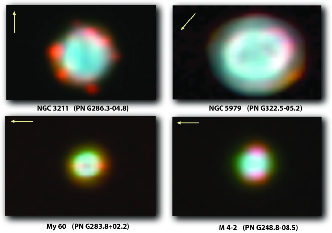
Figure 1: Narrow band continuum-subtracted image composites of our PNe derived from the WiFeS data cubes. The field size of each image is 25″x 38″. The yellow arrow denotes the direction of north in each image. The colour coding of these images is He II $\lambda 4686$ (blue), H$\beta$ (green) and [N II] $\lambda 6583$ (red), and they are presented on a square root stretch to bring out the fainter features. Each image has been boxcar smoothed by 1 spaxel or 1.0″. to remove sharp spaxel boundaries. Note that all objects have only fragmentary shells of [N II] emission, which indicates that all four objects are optically thin to the escape of ionising radiation.

2.4 Global Spectra

In order to build a detailed photoionisation model of the PN, a mean spectrum of the whole nebula is required. From the 3-D data cube, we extracted this spectrum using a circular aperture which matched the observed extent of the bright region of the PNe using QFitsView. The residuals of the night sky lines of [O I] $\lambda$5577.3, [O I] $\lambda$6300.3 and [O I]$\lambda$6363.8 were removed by hand. The scaling between the blue and red spectra caused by slight mis-match of the extraction apertures was improved by measuring the total fluxes in the common spectral range between blue and red channels (5500-5700 Å), and applying the scale factor to the red spectrum to match the two measured fluxes.

We measured emission-line fluxes from the final combined, flux-calibrated blue and red spectra of each PN. The line fluxes and their uncertainties were measured using the IRAF splot task and were integrated between two given limits, over a local continuum fitted by eye, using multiple Gaussian fitting for the line profile. We used the Nebular Empirical Abundance Tool (NEAT; Wesson et al. 2012) to derive the reddening coefficients and in the subsequent plasma diagnostics and ionic and elemental abundances calculations. The derived logarithmic reddening coefficients and the H$\beta$ fluxes are given in Table 2, and the complete list of line intensities is given in the appendix in Table 9.

Table 2: Reddening coefficients, observed $H\beta$ fluxes, excitation classes and inferred distances of our sample.

Object	${\bf c(H\beta)}$		Log F$(H\beta)$		EC		Distance (kpc)
	This Paper	Literature	This paper	Literature	(6)	(7)	(8)	(9)
NGC 3211	0.37	0.34(1), 0.32(2), 0.25(3)	-11.12	-11.06(2), -11.39(3)	10.1	9.1	2.61	2.59
NGC 5979	0.40	0.38(1), 0.25(4)	-11.34	-11.23(2), -11.9(5)	10.8	10.1	2.99	2.49
My 60	0.86	0.91(1), 0.95(2), 0.87(4)	-11.83	-11.78(2), -11.8(5)	10.4	8.8	3.76	3.33
M 4-2	0.57	0.37(1)	-11.85	-11.70(5)	9.5	9.0	5.91	5.72

References.: (1) Tylenda et al. (1992);(2) Shaw & Kaler (1989); (3) Milingo et al. (2002); (4) Górny (2014); (5) Acker et al. (1991); (6) Reid & Parker (2010); (7) Meatheringham & Dopita (1991); (8) Ali et al. (2015a); (9) Frew et al. (2016), assuming all objects are optically thin.

3 Determination of physical conditions

3.1 Temperatures and densities

The spectral lines in the sample given in Table 9 allow us to determine the electron densities from the low and medium ionization zones and the electron temperature from the low, medium and high ionization zones. The lines of low ionisation were used to determine the nebular densities from the [S II] $\lambda$6716/$\lambda$6731 and [O II] $\lambda$3727/$\lambda$3729 and the temperatures from [N II] ($\lambda 6548+\lambda 6584$)/$\lambda$5754 line ratios, while in the more highly ionised zones we determine the nebular densities from the [Cl III] $\lambda$5517/$\lambda$5537, [Ar IV] $\lambda$4711/$\lambda$4740 and [Ne IV] $\lambda$4715/$\lambda$4726 line ratios, while the temperature is estimated from the [O III] ($\lambda 4959+\lambda 5007$)/$\lambda$4363 line ratio. For NGC 5979, we also able to determine the nebular temperature from the high ionization line ratio [Ar V] ($\lambda 6435+\lambda 7005$)/$\lambda$4625. The Monte Carlo technique was used by NEAT to propagate the statistical uncertainties from the line flux measurements through to the derived abundances. In Table 3, we list the inferred nebular densities, temperatures and their uncertainties for each object. In addition, we provide comparisons of our results with those which have previously appeared in the literature. In general, we find good agreement with other results.

Table 3 also gives the values of the density and temperature derived from the global photoionisation models which are presented in detail and discussed in Section 6, below.

Table 3: Electron temperatures and densities measured for the PNe sample, and fitted using global photoionisation modelling.

Object	Temperature (K)				Density (cm-3)
	[O III]	[N II]	[S II]	[Ar V]	[S II]	[O II]	[Ar IV]	[Cl III]	[Ne IV]
NGC 3211
Measured:	13937$\pm$ 162	11892$\pm$587			1363$\pm$270	1601$\pm$134	1583.6$\pm$317	1048$\pm$848
Nebular Model:	14810	11910	10910	17040	1370	1684	1464	1538	1310
Ref (1)	13300	10300			1200
Ref (2)	14320
Ref (3)	14000	12500				970
NGC 5979
Measured:	13885$\pm$234	13578$\pm$1217		14375$\pm$902	1470$\pm$320	2034$\pm$261	1342$\pm$503	1342$\pm$503
Nebular Model:	13860	13640	13690	15180	1680	1695	1625	1667	1583
Ref (4)					1549	1585	1862	2570
Ref (5)		$14604^{+15206}_{-14049}$			$509^{+849}_{-240}$
Ref (6)	13100					1410
My 60
Measured:	13665$\pm$229	13411$\pm$688			2098$\pm$215	3009$\pm$706	1763$\pm$472	1637$\pm$945
Nebular Model:	13210	13270	13340	15250	2132	2150	2045	2113
Ref (5)		$13868^{+14412}_{-13324}$			$1510^{+2450}_{-1050}$
M 4-2
Measured:	15170$\pm$186	11084$\pm$380			1662$\pm$78	2178$\pm$235	1537$\pm$486	1164$\pm$864
Nebular Model:	14070	12080	11350	16870	1775	2088	1680	2027	1745

References: (1) Henry et al. (2004); (2) Kaler et al. (1996); (3) Liu & Danziger (1993); (4) Wang et al. (2004); (5) Górny (2014); (6) Kingsburgh & Barlow (1994)

3.2 Excitation classes and distances

The detected emission lines in all objects cover a wide range of ionization states from neutral species such as [O I], all the way up to [Ne V] which requires the presence of photons with greater energy than 97.1 eV. For medium and high excitation classes (EC), above EC=5, the line ratio of He II $\lambda 4686$Å$/H\beta$ provides the best indication of excitation class of the nebula. This line is only present when the central star has an effective temperature, $T_{\rm eff}>85000$K. Based on the analysis of 586 PNe in the Large Magellanic Cloud (LMC), Reid & Parker (2010) compared the three main classification schemes of Aller (1956), Meatheringham & Dopita (1991) and Stanghellini et al. (2002) to estimate the excitation classes of PNe. They noticed that at EC $\geq 5$, the line ratio [O III]$/H\beta$ is not fixed but it increases to some degree with nebular excitation. Therefore they introduced a new method to incorporate both the He II $\lambda 4686$Å$/H\beta$ and [O III]$/H\beta$ line ratios in classifying the EC of the nebula. Here we present (Table 2) the excitation class for the four objects using both methods of Reid & Parker (2010) and Meatheringham & Dopita (1991).

Determining a reliable distance for a planetary nebula is not an easy task. To determine the distance of PN, one should rely first on the individual methods, then on the statistical methods. A summary on the applications, assumptions, limitations, and uncertainties of individual methods was given in Ali et al. (2015a) and Frew et al. (2016). Considering the individual distances in the literature, we found that NGC 3211 and NGC 5979 have each two distance estimates, and My 60 has only one. NGC 3211 has distances of 1.91 kpc (Gathier et al. (1986) - extinction method) and 3.7 kpc (Zhang (1993) - gravity method). The latter technique should be the most reliable in this case. NGC 5979 has distances of 2.0 kpc (Frew et al. (2016) - expansion method) and 5.8 kpc (Zhang (1993) - gravity method). My 60 has a distance of 3.2 kpc (Zhang (1993) - gravity method). On average, Ali et al. (2015a) finds the gravity method overestimates the PN distance by $\sim 25\%$ compared to other methods. It is also obvious here that a large variation exists between the various distance estimates of NGC 3211 and NGC 5979. This discrepancy in distance estimates commonly appears, not only among different methods, but sometimes between different authors using the same method (Ali et al., 2015a). Lacking trusted individual distances, e.g. trigonometric or cluster membership distances, for any of the sample, we rely initially on the statistical methods. For each PN in our sample, we derived two statistical distances which are given in Table 2. The first value was deduced from the distance scale of Ali et al. (2015a), while the second value was taken from that of Frew et al. (2016). We find small distance variations between both distance scales ($\sim 1\%-17\%$), assuming that all objects are optically thin PNe (Table 2). In this paper we have adopted the nebular distances derived from the distance scale of Ali et al. (2015a). These distances may be compared with those derived in Section 6.2 (below).

On the basis of these distances, we derived absolute luminosities $L_{\rm H\beta}$: $1.44\times 10^{34}$ erg s^-1, $1.24\times 10^{34}$ erg s^-1, $1.79\times 10^{34}$ erg s^-1 and $2.20\times 10^{34}$ erg s^-1 for NGC 3211, NGC 5979, My 60, and M 4-2 respectively.

3.3 Ionic and elemental abundances

Applying the NEAT, ionic abundances of nitrogen, oxygen, neon, argon, chlorine and sulfur were calculated from collisional excitation lines (CEL), while helium and carbon were calculated from optical recombination lines (ORL) using the temperature and density appropriate to their ionization potential. When several lines from a given ion are present, the ionic abundance adopted is found by averaging the abundances from each ion and weighted according to the observed intensity of the line. The total abundances were calculated from ionic abundances using the ionization correction factors (ICF) given by Kingsburgh & Barlow (1994), to correct for unseen ions.

The total helium abundances for all objects were determined from He⁺/H and He²⁺/H ions. The total carbon abundances were determined from C²⁺/H and C³⁺/H ions for all objects, except My 60 which is determined from C²⁺/H ion only, using ICF (C) = 1.0.

None of the objects studied here has He/H $\geq 0.125$ and/or N/O $\geq 0.5$. Therefore, they can not be classified as a Type I according to the original classification scheme proposed by Peimbert (1978). This probably implies that their progenitor stars had lower initial masses ($M<4M_{\odot}$). According to the derived chemical compositions of the objects, they will most likely to be classified as Types II and III. These types of PNe have abundances which more nearly reflect the properties of the interstellar medium out of which their central stars have been formed, particularly with respect to those chemical elements that are not contaminated by the evolution of intermediate mass stars, such as oxygen, neon, sulphur and argon. The He/H, N/H and N/O abundances in NGC 3211 and NGC 5979 are consistent with Type IIa PNe (Quireza et al., 2007). The Galactic vertical height (z $\leqslant$ 1 kpc) and peculiar velocity ($\leqslant$ 60 km$s^{-1}$) of NGC 3211 confirm that it is probably a member of Galactic thin disk. The chemistry of My 60 and M 4-2 is consistent with Type IIb/III PNe, both nebulae have Galactic vertical heights less than 1 kpc, but peculiar velocities larger than 60 km s^-1. Therefore we suggest that both objects are of Type III PNe, which are usually located in the Galactic thick disk. These results are consistent with that of Fogel et al. (2003) and Girard et al. (2007) where none of WELS are associated with Type I PNe.

Tables 4 and 5, compare the abundance determinations of the four objects with those obtained by our detailed global photoionisation models and with those given by other authors.

Table 4: Abundances derived from the NEAT and MAPPINGS codes for NGC 3211 and NGC 5979. Model I refers to the total abundances in the photoioionsation model, while model II refers to gas phase abundances in the same model.

	NGC 3211							NGC 5979
Element	Neat	Model I	Model II	Ref 1	Ref 2	Ref 3		Neat	Model I	Model II	Ref 4
He/H	1.06E-1$\pm$2.7E-3	1.10E-1	1.10E-1	1.10E-1		1.17E-1		1.10E-1$\pm$3.9E-3	1.10E-1	1.10E-1	1.11E-1${}^{+1.17{\rm E}-1}_{-1.05{\rm E}-1}$
C/H	1.20E-3$\pm$6.7E-5	1.34E-3	8.64E-4					2.05E-3$\pm$1.3E-4	1.84E-3	1.19E-3
N/H	1.15E-4$\pm$9.9E-6	7.96E-5	6.62E-5	1.63E-4				1.38E-4$\pm$1.2E-5	2.81E-5	2.33E-5	6.70E-5${}^{+7.62{\rm E}-5}_{-5.62{\rm E}-5}$
O/H	4.43E-4$\pm$2.0E-5	4.60E-4	2.97E-4	8.38E-4	5.00E-4	8.77E-4		4.55E-4$\pm$3.0E-5	6.21E-4	3.74E-4	3.44E-4${}^{+4.06{\rm E}-4}_{-2.87{\rm E}-4}$
Ne/H	9.30E-5$\pm$3.9E-6	7.82E-5	7.82E-5	1.31E-4	1.38E-4			5.63E-5$\pm$7.8E-6	6.05E-5	6.05E-5	5.75E-5${}^{+6.59{\rm E}-5}_{-5.13{\rm E}-5}$
Ar/H	1.90E-6$\pm$9.6E-8	1.60E-6	1.60E-6	6.33E-6				2.17E-6$\pm$1.3E-7	2.17E-6	2.17E-6	2.27E-6${}^{+2.48{\rm E}-6}_{-2.03{\rm E}-6}$
K/H		8.07E-7	8.07E-7
S/H	6.18E-6$\pm$4.83E-7	5.41E-6	5.41E-6	4.40E-6	1.34E-5			8.48E-6$\pm$7.3E-7	3.92E-6	3.92E-6	5.32E-6${}^{+5.92{\rm E}-6}_{-4.62{\rm E}-6}$
Cl/H	1.46E-7$\pm$1.44E-8	5.40E-7	1.45E-7	4.52E-7				1.90E-7$\pm$1.6E-8	4.20E-7	1.13E-7	9.30E-6${}^{+1.13{\rm E-5}}_{-6.87{\rm E-6}}$
Fe/H			6.80E-8							2.97E-8
N/O	0.26	0.17	0.23					0.23	0.06	0.08

Note: The abundances of K and C elements in models I & II were calculated from [K IV] and C II $\lambda$4267 emission lines, respectively. References: (1) Henry et al. (2004); (2) Maciel & Quireza (1999); (3) Liu & Danziger (1993); (4) Górny (2014).

Table 5: Abundances derived from the NEAT and MAPPINGS codes for My 60 and M 4-2. Model I refers to the total abundances, while model II refers to gas phase abundances in the same model.

	My 60					M 4-2
Element	Neat	Model I	Model II	Ref 1		Neat	Model I	Model II	Ref 2
He/H	1.10E-1$\pm$3.9E-3	1.10E-1	1.10E-1	1.10E-1${}^{+1.16{\rm E}-1}_{-1.03{\rm E}-1}$		9.81E-2$\pm$2.7E-3	1.04E-1	1.04E-1	1.14E-1
C/H	6.31E-4$\pm$1.2E-4	1.16E-3	7.50E-4			2.58E-3$\pm$1.2E-4	1.71E-3	1.19E-3
N/H	6.85E-5$\pm$7.5E-6	4.98E-5	4.14E-5	5.11E-5${}^{+6.40{\rm E}-5}_{-4.17{\rm E}-5}$		5.73E-5$\pm$3.8E-6	5.74E-5	5.24E-5	1.97E-4
O/H	3.15E-4$\pm$2.0E-5	4.60E-4	2.97E-4	3.15E-4${}^{+3.80{\rm E}-5}_{-2.62{\rm E}-4}$		2.40E-4$\pm$1.1E-5	2.08E-4	1.62E-4	4.70E-4
Ne/H	6.20E-5$\pm$3.9E-6	6.81E-5	6.81E-5	6.02E-5${}^{+6.92{\rm E}-5}_{-5.24{\rm E}-5}$		4.85E-5$\pm$2.1E-6	4.26E-5	4.26E-5
Ar/H	1.59E-6$\pm$1.1E-7	2.20E-6	2.20E-6	1.68E-6${}^{+1.86{\rm E}-6}_{-1.48{\rm E}-6}$		9.27E-7$\pm$1.5E-8	8.30E-7	8.30E-7
K/H			1.01E-7				1.90E-7
S/H	4.92E-6$\pm$4.7E-7	4.50E-6	4.50E-6	4.33E-6${}^{+5.10{\rm E}-6}_{-3.66{\rm E}-6}$		2.35E-6$\pm$1.5E-7	3.80E-6
Cl/H	1.20E-7$\pm$1.4E-8	4.01E-7	1.10E-7	8.33E-6${}^{+1.04{\rm E}-5}_{-6.34{\rm E}-6}$		4.48E-8$\pm$4.1E-9	9.31E-8
Fe/H			9.62E-8					6.75E-8
N/O	0.22	0.11	0.14			0.24	0.22	0.26

Note: The abundances of K and C elements in models I & II were calculated from the [K IV] and C II $\lambda$4267 emission lines, respectively. References: (1) Górny (2014); (2) Kaler et al. (1996).

4 Expansion and radial velocities

The expansion velocity is an essential quantity to determine in order to understand nebular evolution. We used three emission lines ([S II], [N II], [Ar V]) that all lie in the red part of the WiFeS spectrum, and are consequently observed at higher spectral resolution (R=7000) than the blue spectra (R=3000). These lines were used to determine the nebular expansion velocity $V_{\rm exp}$ for each object. The full width at half maximum (FWHM) of each line was measured using the IRAF splot task. The full width was corrected for instrumental and thermal broadening to derive the expansion velocity using the following formula (Gieseking et al., 1986);

$$V_{\rm exp}=0.5\left[w^{2}_{\rm obs}-w^{2}_{\rm inst}-8(\ln 2)kT_{e}/m\right]^{1/2}$$ (1)

where $w_{\rm obs}$ is the observed FWHM of the measured line, $w_{\rm inst}$ is the instrumental FWHM, $k$ Boltzmann’s constant, $T_{e}$ is the nebular temperature, and $m$ the atomic mass of the species emitting the measured line. The results are given in Table 6. As expected from the ionisation stratification of these PNe, the measured expansion velocity decreases with increasing ionisation potential of the ion. Apparently, there are no previous attempts to measure the expansion velocity of M 4-2. NGC 3211 has measured velocities of 26.5 kms^-1, 31.0 kms^-1 and 21.1 kms^-1 using the [O III], [O II] and He II emission lines, respectively (Meatheringham et al., 1988). Our derived expansion velocities for NGC 3211 in the [N II] and [S II] are smaller than those of Meatheringham et al. (1988), except for He II line. This may be attributed to the derivation of the expansion velocity from an integrated spectrum over the whole object, while other authors usually derive the expansion velocity at a certain nebular position using long slit spectra. In the study of Meatheringham et al. (1988), they measured the maximum velocity for asymmetric objects by set the spectrograph slit along the nebular long axis. It is clear also from the NGC 3211 colour image in Figure 1 that the [N II] emission is strongly concentrated in blobs located in the outer regions of the nebula. Hajian et al. (2007) gave an equatorial expansion velocity of 18 kms^-1 for NGC 5979 derived from long slit spectra in the [O III] emission line. This value is consistent with our measurements and slightly smaller than that derived from [S II] and [N II] emission lines, due to the higher ionisation potential of the [O III] line. Schönberner et al. (2005) provided two expansion velocities for the rim of My 60. They derived $V_{\rm exp}$ = 23.1 kms^-1 and 23.7 kms^-1 from [O III] and [N II] emission lines, respectively. The latter one is in good agreement with our derived value.

The systemic velocities $RV_{\rm sys}$ of the sample were measured using the IRAF external package RVSAO. A weighted mean radial velocity was calculated for each object using $H\alpha$, [N II], and [S II] emission lines. The heliocenteric correction was taken from the image header, to derive the heliocentric radial velocity $RV_{\rm hel}$ for each object. The results were listed in Table 6. The value of NGC 3211 is in good agreement with Durand et al. (1998) and Schneider & Terzian (1983). The radial velocity of NGC 5979 is higher than that derived by Schneider & Terzian (1983), $RV_{\rm hel}=23\pm 3.0$, which was taken originally from the low dispersion spectra of Campbell & Moore (1918). Therefore our larger value of $RV_{\rm hel}$ for NGC 5979, compared to that of Schneider & Terzian (1983), may be attributed to the different spectral resolution as well as to the fact that we derived the radial velocity from the integrated spectrum over the whole object, while other value was derived from a particular nebular position.

Table 6: Radial and expansion velocities of the sample.

Object	$RV_{\rm hel}$ (km/s)		Vexp (km/s)
	This paper	Literature	[S II]	[N II]	[Ar V]
NGC 3211	-21.8$\pm$3.5	-22.3$\pm$1.6(1), -22.5$\pm$2.8(2)	23.6	22.0	10.3
NGC 5979	30.4$\pm$3.5	23.0$\pm$3.0(1)	20.7	22.4	11.8
My 60	42.2$\pm$3.0		24.2	24.1	$<$ 10
M 4-2	119.1$\pm$4.7		25.9	25.5	9.3

References. : (1) Durand et al. (1998); (2) Schneider & Terzian (1983)

5 What are the central stars?

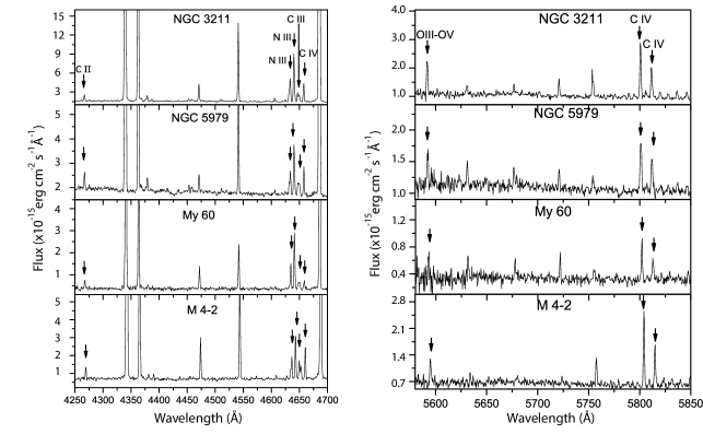
Figure 2: Characteristic emission lines generally used to classify central stars as of the WELS type, as seen in our PNe sample.

Figure 3: Narrow band continuum-subtracted image composites of our PNe in the recombination lines of C IV $\lambda 5801$ (blue), N III $\lambda 4641$ (green), [N II] $\lambda 6583$ (red). As in Figure 1, they are presented on a square root stretch to bring out the fainter features and boxcar smoothed by 1 spaxel or 1.0 arc sec. to remove sharp spaxel boundaries. The arrow shows the direction of north. No trace of a central star is seen in any object. Instead, the recombination line emission of C IV and N III is - in each case - entirely of nebular origin.

Of the over 3000 Galactic PNe currently known (Frew & Parker, 2010), only 13 % of their stellar nuclei have been spectroscopically identified (Weidmann & Gamen, 2011). According to the observed atmospheric spectra of the CSs of PNe, Mendez (1991) has assigned two types. In the first type hydrogen is the prevalent element (H-rich), while the second type is relatively free of hydrogen and the spectra are dominated by lines of helium and carbon elements (H-deficient).

In general, the H-deficient type can be divided into three main groups. The first group, the [WR] group, shows spectra with strong and broad emission lines mainly from He, C, and O, similar to the Wolf-Rayet stars of population I. This group was divided into three subgroups: [WCL], [WCE], and [WO], according to the ionization stages of the element dominating the atmosphere (Crowther et al., 1998; Acker & Neiner, 2003). The second group, PG1159, is composed of pre-white dwarfs that have mainly absorption lines of He II and C IV in their spectra (Werner et al. 1997). The third group, [WC]-PG 1159, includes objects with similar optical spectra to the PG1159 stars, but have strong P Cygni lines in the UV (e.g. N V $\lambda$1238 and C IV $\lambda$1549).

Tylenda et al. (1993) presented the analyses of extensive observations of a set of 77 emission-line CSs. About half of this set were classified as [WR] stars and the other half exhibited emission lines at the same wavelengths as [WR] stars, but having weaker intensities and narrower line widths. These they named “weak emission-line stars” (WELS). The spectra of the WELS show the carbon doublet, C IV $\lambda$5801 and $\lambda$5812 and the $\lambda$4650 feature which is a blend of N III $\lambda$4634 and $\lambda$4641, C III $\lambda$4650, and C IV $\lambda$4658. Furthermore the spectra of WELS are highly ionized to the degree that the C IV $\lambda$$\lambda$5801, 5812 doublet is strong but the C III $\lambda$5696 line is either very weak or absent. Based on the analysis of the optical spectra of 31 WELS, Parthasarathy et al. (1998) found that the spectrum of a WELS is very similar to those of the [WC]-PG1159 and PG1159 stars. As pointed out in the introduction, they suggested that an evolutionary sequence exists connecting the [WC] central stars of PNe to the PG1159 pre-white dwarfs: [WC late] $\rightarrow$ [WC early] $\rightarrow$ WELS = [WC]-PG1159 $\rightarrow$ PG1159. Based on the UV spectra of the WELS, Marcolino et al. (2007) disagreed with Parthasarathy et al. (1998), and instead claimed that the WELS are distinct from [WC]-PG1159 stars. They noticed that WELS type presented P Cygni features and most of their terminal velocities lie in the range from $\sim$1000-1500 km s^-1, while [WC]-PG1159 stars have much higher values of $\sim$3000 km s^-1. In addition, they found that the [WC]-PG1159 stars are characterised by several intense P Cygni emission in the $\sim$1150-2000Å wavelength interval, most notably N V $\lambda$1238, O V $\lambda$1371, and C IV $\lambda$1549, while in the WELS O V $\lambda$1371 is either very weak or absent. Furthermore, Parthasarathy et al. (1998) and Marcolino & de Araújo (2003) find some absorption lines in the optical spectra of WELS such as He II $\lambda$4541 and $\lambda$5412 indicating that any stellar wind is not as dense as in the case of [WR] stars.

Hajduk et al. (2010) claimed that not all WELS spectral type are H-deficient as [WR] stars, but some may be H-rich despite having emission lines. Recently, Weidmann et al. (2015) have observed and studied 19 WELS from the total of 72 objects known in literature. The high quality spectra of these objects show a variety of spectral types, where 12 of them have H-rich atmospheres, with different wind densities and only 2 objects seem to be H-deficient. They were not able to decide on the spectral type of the remaining objects, but they concluded that these objects are not [WR] stars. According to the above results, they claimed that “the denomination WELS should not be taken as a spectral type, because, as a WELS is based on low-resolution spectra, it cannot provide enough information about the photospheric H abundance”.

Three objects of our sample have previously been associated with the WELS type: NGC 5979, M 4-2 (Weidmann & Gamen, 2011) and My 60 (Górny, 2014). Due to the low spectral resolution, the components of C+N $\lambda$4650 feature were not resolved in the spectra presented by Weidmann & Gamen (2011) - their Figure 11 and Górny (2014) - their Figure C.2. Furthermore the components of the doublet C IV centred at 5805Å were not resolved in the spectra given by Weidmann & Gamen (2011) - their figure 11. In Figure 2, we illustrate our observations of the characteristic WELS emission lines seen in all four of our objects. Here, to simulate the effect of observing with a long-slit spectrograph, we extracted these spectra by taking a circle of 2″radius around the geometric centre of each object. In general, the spectra of all nebulae roughly show similar emission lines, generally identified to be of the WELS class; C II at 4267Å, N III at 4634Å and 4641Å , C III at 4650Å (here resolved into its two components at 4647Å and 4650Å), C IV at 4658Å, O III-O V at 5592Å, and finally, C IV at 5801Å and 5812Å.

Górny (2014) noticed that it was possible that - as in the case of NGC 5979 - the CS spectrum can “mimic” the WELS type. They found that the key CS emission features of WELS type (C II at 4267Å, N III at 4634Å and 4641Å, C III at 4650Å, C IV at 5801Å and 5812Å) appear in a spatially extended region in the 2D spectra of NGC 5979, and therefore, they are of nebular rather than stellar origin.

To test whether the CSs in our objects were real WELS-type, or simply “mimics”, we constructed continuum-subtracted images in the brightest recombination lines C IV $\lambda 5801$ and N III $\lambda 4641$, and formed colour composites using the procedure described in Section 2.3. The result is shown in Figure 3. From this is evident that the recombination lines are formed in the nebula, and that the spatial separation of the C IV, N III and [N II] emission is entirely consistent with ionisation stratification. We therefore conclude that, in every case the emission is entirely of nebular origin, and that the WELS classification is spurious for these objects.

Certainly, the CSs are detected, but if not of the WELS type, what could they be? In order to examine this, we need to carefully remove the nebular emission. This was possible in three cases; NGC 3211, NGC 5979 and My 60. The result is shown in Figure 4 for NGC 5979. There are broad Balmer absorption features present in the blue continuum of the star, and three stellar emission lines, O VI $\lambda\lambda 3811.3,3834.2$ and O V $\lambda 4664.4$ . The presence of broad Balmer absorption in the CS proves the presence of H in the atmosphere, and establishes that the CS is likely to be H-burning. However, the source of the narrow O VI and O V lines remains uncertain. Being narrow, they most likely have their origin in or close to the photosphere, rather than in the wind. We tentatively classify this star, following the CS classification scheme of Mendez (1991), as O(H)-Type. These features clearly originate in the central star as can be seen from the continuum-subtracted emission line maps shown as thumbnail images in Figure 4. In the case of NGC 3211 and My 60, only the O VI $\lambda\lambda 3811.3,3834.2$ doublet was identified in their CSs, but this is sufficient to classify these stars as also belonging to the O(H)-Type. In M 4-2 only a faint blue continuum could be identified as coming from the central star, so this star remains without classification.

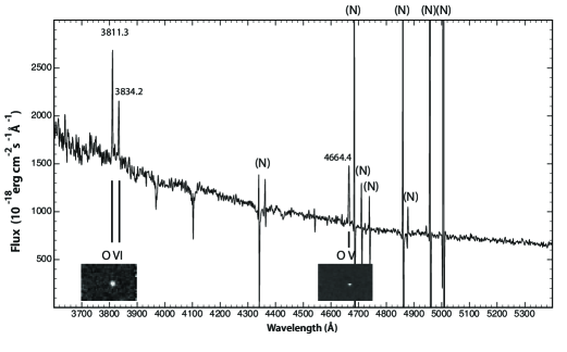
Figure 4: The nebular subtracted spectrum of the central star in NGC 5979 (showing the full WiFeS image field). Emission lines of O VI and O V are clearly detected in the central star, as indicated in the monochromatic thumbnail images shown in the lower part of the figure. The features marked (N) are improperly subtracted nebular features. There are broad Balmer absorption features present in the blue continuum of the star.

6 Self-consistent photoionization modelling

Integral field spectroscopy of PNe in our Galaxy presents an ideal opportunity to build fully self-consistent photoionisation models. Not only can a global spectrum be extracted which is directly comparable to the theoretical model, but we are able to use the size and morphology to constrain the photoionisation structure and inner and outer boundaries of the nebula. In addition, we can directly compare measured electron temperatures and densities in the different ionisation zones to constrain the pressure distribution within the ionised material. In this section, we describe how such self-consistent photoionisation modelling can provide a good description to all these parameters, while at the same time enabling us to derive chemical abundances, to derive distances, and to place the central stars on the H-R diagram. We refer the reader to earlier work of this nature on the PN NGC 6828 by Surendiranath & Pottasch (2008).

We have used the Mappings 5.0 code (Sutherland et al. 2015, in prep.) . Earlier versions of this code have been used to construct photoionisation models of H II regions, PNe, Herbig-Haro Objects, supernova remnants and narrow-line regions excited by AGN. This code is the latest version of the Mappings 4.0 code earlier described in (Dopita et al., 2013), and includes many upgrades to both the input atomic physics and the methods of solution.

We choose for the initial abundance set in the models a value of 0.8 times local galactic concordance (LGC) abundances based upon the Nieva & Przybilla (2012) data on early B-star data. The Nieva & Przybilla (2012) data provide the abundances of the main coolants, H, He, C, N. O, Ne, Mg, Si and Fe and the ratios of N/O and C/O as a function of abundance. For the light elements we use the Lodders et al. (2009) abundance, while for all other elements the abundances are based upon Scott et al. (2015a); Scott et al. (2015b) and Grevesse et al. (2010). The individual elemental abundances are then iterated from this initial set.

The elemental depletions onto dust grains must be taken into account. Not only do these remove coolants from the nebular gas, but in PNe they are also an important source of photoelectric heating (Dopita & Sutherland, 2000). For the depletion factors we use the Jenkins (2009) scheme, with a base depletion of Fe of 1.5 dex. For the dust model, we use a standard Mathis et al. (1977) dust grain size distribution.

For the spectral energy distribution of the CS, we use the Rauch (2003) model grid, which provide metal-line blanketed NLTE model atmospheres for the full range of parameters appropriate to the CSs of PNe. Our initial estimate uses the $\log g=6.0$ models.

The pressure in the ionised gas is an important parameter. In the modelling we have used the isobaric approximation (which includes any effect of radiation pressure), and we have matched the pressure to fit the electron densities derived from observation, given in Table 3, above. In this table we have also listed the electron densities (and electron temperatures) returned from our “best fit” models. Generally speaking, the agreement is good to a few percent.

It is clear from the optical morphology given in Figure 1 that all four of our nebulae are optically thin to the escape of ionising photons, some more than others. We therefore developed a 2-component model consisting of the weighted mean of an optically-thin component and an optically-thick component.

In addition to the chemical abundance set, the gas pressure, and the fraction of optically-thin gas $F$, the parameters which determine the relative line intensities in the model are the stellar effective temperature $T_{\rm eff}$, the ionisation parameter at the inner boundary of the PNe, $U_{\rm in}$ and the fraction of the Strömgren radius ($R_{\rm S}$) at which the outer boundary of the optically-thin component is located $f_{\rm S}=R_{\rm out}/R_{\rm S}$. The objective of the modelling is to produce a unique solution to each of these variables.

The strength of the emission lines of low excitation such as [N II], [S II] and [O II] is very sensitive to the fraction of optically-thick gas present, and these therefore provide an excellent constraint on $F$. A further constrain on $F$ is furnished by the [O III]/H$\beta$ ratio, since this first increases, and then sharply decreases as the nebula becomes increasingly optically-thin. All four of our PNe are located close to the maximum in the [O III]/H$\beta$ ratio that is observed in PNe. In addition, the helium and hydrogen excitation as measured by the He II$\lambda 4686$/He l$\lambda 5876$ and the He l$\lambda 5876$/H$\beta$ ratios is sensitive to both $T_{\rm eff}$ and $U_{\rm in}$. For a given $f_{\rm S}$, there is a narrow strip of allowed solutions with $\log U_{\rm in}$ falling as $T_{\rm eff}$ rises.

In order to measure the goodness of fit of any particular photoionisation model, we measure the L1-norm for the fit. That is to say that we measure the modulus of the mean logarithmic difference in flux (relative to H$\beta$) between the model and the observations viz.;

$${\rm L1}={\Sigma}_{n}\left|\log\left[{F_{n}({\rm model})}\over{F_{n}({\rm obs.)}}\right]\right|/n,$$ (2)

where n is the number of lines being considered in the fit. This weights fainter lines equally with stronger lines, and is therefore more sensitive to the values of the input parameters. (By themselves, the stronger lines would not provide sufficient constraints on the variables of the photoionisation models, and the signal to noise in our spectra is very adequate to measure these fainter lines with sufficient accuracy - see Table A1). Typically, we simultaneously fit between 27 and 35 emission lines.

For a given $f_{\rm S}$ we ran an extensive grid of models in $\log U_{\rm in}$ and $T_{\rm eff}$, and searched for the region where the L1-norm was minimised at the same time as the helium excitation matching the observed value. When this point was identified, we iterated the abundance set in a restricted $\log U_{\rm in}$ and $T_{\rm eff}$ range to improve on the L1-norm. Typically, we could reduce this to about 0.05 dex, the error being mostly dominated by a few lines for which apparently the models are inadequate. These are discussed below.

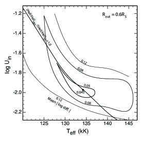
Figure 5: The best fit solution for M 4-2 is shown here on the $\log U_{\rm in}$ and $T_{\rm eff}$ plane. We seek to minimise the L1-norm (contours), here given by fitting 35 lines, while simultaneously matching the He II, He I and H II excitation to that observed in the nebula.

In Figure 5 we show the solution in the case of M 4-2. For this model, we also provide in Figure 6 a comparison between the theoretical model (including the central star) and the observations. Here we have matched the resolution of the theoretical spectrum to that of the observations, as best as we can. Note that the flux scale is logarithmic and covers nearly 4 dex. The Mappings 5.0 code does not provide predictions for the higher Balmer and He II $n=5$ series, as these become sensitive to the density. Nor does the code predict the intensities of the recombination lines of highly ionised species such as the N III, C III, C IV, O V and O VI lines discussed above. This is simply because the appropriate recombination coefficients and other atomic data are not available for these transitions in these ions. Normally the recombination coefficients into the excited states would be estimated from the photoionization cross-sections using the Milne relation. However, there are no published estimates of photoionization cross-sections from these excited states. Furthermore, the population of the upper level is also determined by the cascade from more highly excited states, as well as by collisional contributions from the lower levels. Finally, for some excited levels radiative transfer effects (e.g. case A or B) can make large differences to the predicted recombination line strengths, and UV pumping into upper states followed by radiative cascade into the upper state of the transition being considered can also be very important. Apart from these issues, which regrettably specifically affect the characteristic WELS recombination lines, the overall fit of the model to the observation is excellent.

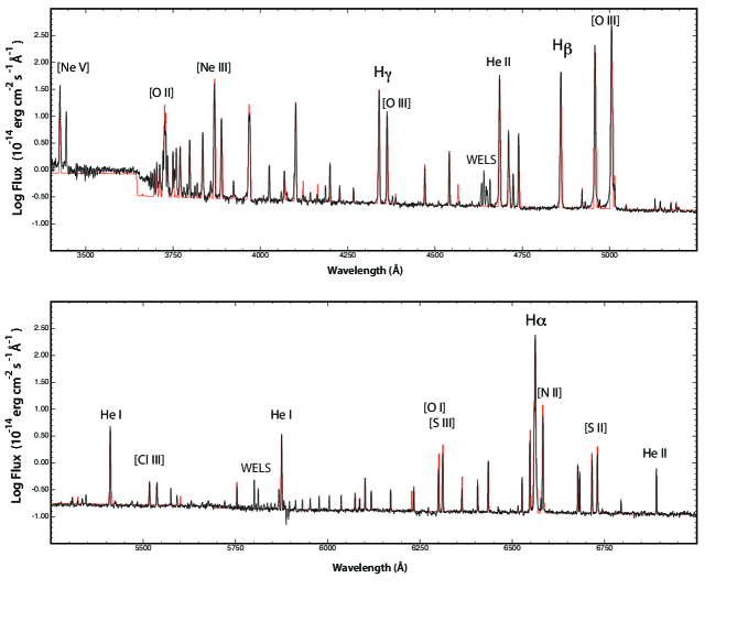
Figure 6: The comparison between the observed (dereddened) global spectrum of M 4-2 (PN G248.8-08.5) (black) and the best fit Mappings 5.0 photoionisation model (red). Some of the principal emission lines are identified. Note the excellent agreement between the observed and the theoretical nebular + stellar continuum, which is only possible when the observed spectrum has been correctly de-reddened.

The derived parameters for the“best fit” final models are as follows:

	log P/k	$F$	$f_{\rm S}$	log $U_{\rm in}$	$T_{\rm eff}$
	cm-3K				kK
NGC 3211	7.63	0.992	0.72	-1.95	145
NGC 5979	7.62	1.00	0.64	-1.60	160
My 60	7.72	1.00	0.60	-1.55	130
M 4-2	7.73	0.935	0.60	-1.90	134

In Table 7, we present a comparison of the observed and modelled line intensities of the lines used in the fitting. Overall the agreement between the model and the observations is good. However, we note a systematic effect that limits the minimum value of the L1-norm. Although the predicted [Ne III] line intensities are satisfactory, the [Ne V] lines are too weak with respect to the [Ne IV] lines, while at the same time the [Ar V] lines are too strong with respect to the [Ar IV] lines. The ionisation potential of Ne III is 63.45eV that of Ne IV is 97.12eV, and the ionisation potential of Ar IV is 59.81eV. These are all high, but in the same general range. Thus, the differences between the predictions and the observations cannot probably be ascribed to differences in the input ionising spectra, but are more likely caused by errors in the charge exchange reactions rates used by the code, which will affect the detailed ionisation balance in the nebula.

Table 7: Line fluxes, relative to H$\beta=100$, from photoionisation models compared with those observed in NGC 3211, NGC 5979, My 60, and M 4-2.

		NGC 3211		NGC5979		My60		M 4-2
Lab (Å)	ID	Model	Observed	Model	Observed	Model	Observed	Model	Observed
3425.88	[Ne V]	45.23	71.4$\pm$2.95	54.31	58.6$\pm$3.49	21.44	26.2$\pm$1.60	19.5	61.4$\pm$2.44
3726.03	[O II]	33.32	17.4$\pm$0.66	18.2	3.4$\pm$0.19	15.10	5.2$\pm$0.36	15.34	11.8$\pm$0.43
3728.82	[O II]	24.3	12.4$\pm$0.47	12.2	2.3$\pm$0.13	10.00	3.0$\pm$0.20	9.75	7.5$\pm$0.32
3770.63	HI 11-2	3.89	4.4$\pm$0.26	3.96	3.6$\pm$0.19	3.98	3.6$\pm$0.25	3.84	3.9$\pm$0.17
3835.39	HI 9-2	7.19	8.5$\pm$0.31	7.30	7.3$\pm$0.39	7.34	7.8$\pm$0.43	7.09	7.7$\pm$0.32
3868.76	[Ne III]	173.7	112.4$\pm$4.1	62.44	58.4$\pm$3.12	109.6	90.3$\pm$4.96	86.30	65.3$\pm$2.34
3889.06	HI 8-2	10.34	16.4$\pm$0.60	10.49	11.5$\pm$0.62	10.55	15.8$\pm$0.85	10.2	14.5 $\pm$0.52
3967.47	[Ne III]	52.35	36.5$\pm$1.30	16.8	17.5$\pm$0.91	33.02	22.9$\pm$1.24	26.01	15.9 $\pm$0.56
3970.08	HI 7-2	15.68	15.8$\pm$0.56	15.89	14.3$\pm$0.75	15.99	15.3$\pm$0.80	15.46	15.5 $\pm$0.54
4068.60	[S II]	1.01	1.8$\pm$0.10	0.20	1.3$\pm$0.07	0.20	2.0$\pm$0.16	0.34	2.4$\pm$0.10
4076.35	[S II]	0.32	0.4$\pm$0.04	0.07	0.1$\pm$0.02	0.06	…	0.11	…
4267.14	C II	0.15	0.5$\pm$0.05	0.80	0.8$\pm$0.05	0.55	0.6$\pm$0.12	0.90	0.9$\pm$0.08
4340.47	HI 5-2	46.98	49.2$\pm$1.52	47.11	44.4$\pm$2.05	47.16	48.3$\pm$2.30	47.05	47.2 $\pm$1.47
4363.21	[O III]	22.75	25.1$\pm$0.81	14.78	14.7$\pm$0.70	18.01	18.9$\pm$0.92	14.91	17.6 $\pm$0.56
4471.50	He I	1.98	1.8$\pm$0.10	0.70	0.8$\pm$0.05	2.11	2.2$\pm$0.17	1.32	1.3$\pm$0.12
4541.59	He II	2.65	2.9$\pm$0.16	3.59	3.7$\pm$0.17	2.68	2.9$\pm$0.18	0.88	2.9$\pm$0.11
4685.70	He II	86.21	85.3$\pm$2.52	105.1	105.5$\pm$4.67	78.48	80.4$\pm$3.59	84.93	83.8$\pm$2.47
4711.26	[Ar IV]	8.20	11.0$\pm$0.33	8.56	14.2$\pm$0.63	7.17	10.7$\pm$0.47	5.46	7.5$\pm$0.28
4714.50	[Ne IV]	0.68	1.5$\pm$0.08	0.32	1.2$\pm$0.05	0.34	…	1.86	1.0$\pm$0.09
4724.89	[Ne IV]	1.24	2.0$\pm$0.11	0.52	1.9$\pm$0.08	0.57	1.3$\pm$0.10	1.20	1.4$\pm$0.13
4740.12	[Ar IV]	6.90	9.6$\pm$0.28	7.45	12.1$\pm$0.53	6.46	9.4$\pm$0.41	6.90	6.5$\pm$0.24
4861.33	HI 4-2	100.0	100.0$\pm$0.0	100.0	100.0$\pm$0.0	100.0	100.0$\pm$0.0	100.0	100.0$\pm$0.0
4958.91	[O III]	399.1	528.5$\pm$14.6	312.0	304.0$\pm$12.7	396.0	422.6$\pm$17.7	237.7	304.0$\pm$8.4
5006.84	[O III]	1153.9	1512$\pm$42	901.8	905.8$\pm$37	1145.0	1184.9$\pm$47	687.0	870.8$\pm$24
5411.52	He II	6.07	6.3$\pm$0.17	8.26	8.6$\pm$0.33	6.17	6.3$\pm$0.24	2.02	6.3$\pm$0.21
5517.71	[Cl III]	1.0	1.0$\pm$0.10	0.50	0.5$\pm$0.03	0.49	0.5$\pm$0.05	0.43	0.4$\pm$0.04
5537.87	[Cl III]	0.90	0.9$\pm$0.09	0.48	0.5$\pm$0.03	0.51	0.5$\pm$0.05	0.42	0.4$\pm$0.04
5875.66	He I	5.74	4.8$\pm$0.13	2.02	2.0$\pm$0.06	6.14	6.2$\pm$0.18	3.86	3.9$\pm$0.10
6086.97	[Fe VII]	0.11	0.1$\pm$0.02	0.09	0.1$\pm$0.00	0.10	0.1$\pm$0.01	0.10	0.1$\pm$0.02
6101.83	[K IV]	0.53	0.5$\pm$0.05	0.70	0.7$\pm$0.03	0.6	0.5$\pm$0.02	0.50	0.5$\pm$0.02
6300.30	[O I]	0.20	0.2$\pm$0.02	0.04	…	0.02	…	0.73	0.8$\pm$0.02
6312.06	[S III]	8.30	3.2$\pm$0.09	1.82	1.8$\pm$0.05	2.21	1.6$\pm$0.05	2.75	1.8$\pm$0.03
6363.78	[O I]	0.08	0.1$\pm$0.02	0.01	…	0.01	…	0.24	0.3$\pm$0.03
6433.12	[Ar V]	2.11	1.0$\pm$0.10	3.79	1.7$\pm$0.05	2.07	0.8$\pm$0.03	0.31	1.0$\pm$0.03
6548.05	[N II]	4.22	5.8$\pm$0.17	0.78	0.7$\pm$0.03	1.22	1.1$\pm$0.03	3.72	4.2$\pm$0.07
6560.09	He II	10.38	9.7$\pm$0.28	14.2	12.7$\pm$0.39	10.61	9.5$\pm$0.27	10.2	11.5$\pm$0.19
6562.82	HI 3-2	288.3	286.7$\pm$3.4	284.0	274.7$\pm$4.3	282.1	283.1$\pm$3.1	286.7	278.8$\pm$2.6
6583.45	[N II]	12.43	15.5$\pm$0.45	2.31	2.4$\pm$0.07	3.58	3.5$\pm$0.10	10.92	10.4$\pm$0.17
6678.15	He I	0.93	1.3$\pm$0.13	0.49	0.5$\pm$0.03	1.47	1.6$\pm$0.05	0.90	1.0$\pm$0.02
6683.45	He II	0.53	0.5$\pm$0.05	0.72	0.8$\pm$0.04	0.54	0.6$\pm$0.02	0.5	0.6$\pm$0.03
6716.44	[S II]	3.90	2.7$\pm$0.15	0.68	0.6$\pm$0.03	0.59	0.6$\pm$0.02	0.89	1.3$\pm$0.02
6730.82	[S II]	4.86	3.2$\pm$0.10	0.93	0.7$\pm$0.03	0.86	0.8$\pm$0.03	1.19	1.7$\pm$0.03
6795.16	[K IV]	0.1	0.1$\pm$0.01	0.21	0.2$\pm$0.01	0.1	0.1$\pm$0.01	0.03	0.1$\pm$0.02
6890.91	He II	0.68	0.7$\pm$0.07	0.92	1.0$\pm$0.05	0.69	0.7$\pm$0.02	0.22	0.8$\pm$0.03
7005.83	[Ar V]	4.61	1.8$\pm$0.10	8.05	3.5$\pm$0.11	4.41	1.8$\pm$0.05	11.97	2.1$\pm$0.05

6.1 Distances from Photoionisation Models

In this section, we will develop on a method to estimate distances based only upon the requirement that the model reproduce both the observed flux and the observed angular size of the PN. The success of this method depends critically on how well we have determined $f_{\rm S}$, since this will in turn determine the relationship between the luminosity of the central star, and the absolute H$\beta$ luminosity of the nebula. Our model, in essence, consists of the application of simple Strömgren theory. For a given electron density $n_{e}$ and nebular radius, $r$, the H$\beta$ luminosity $L_{\rm H\beta}$ is given by:

$$L_{\rm H\beta}\propto n_{e}^{2}r^{3}$$ (3)

and the angular radius $\theta$ is given in terms of the distance $d$, $\theta=r/d$. The reddening-corrected observed H$\beta$ luminosity $F_{\rm H\beta}$ is given by:

$$F_{\rm H\beta}=L_{\rm H\beta}/(4\pi d^{2})$$ (4)

Our photoionisation models give (for any assumed distance and stellar luminosity $L_{*}$) the values of $L_{\rm H\beta},r$ and $n_{e}$, and the observations give us $F_{\rm H\beta}$ and $\theta$, so from these equations we can solve for the distance at which the model predicted angular radius $\theta$ and H$\beta$ flux agree with the observed values. Note that the solution depends critically on the accurate determination of the parameter $f_{\rm S}$, which affects both the absolute flux and the radius of the model, and on $\log P/k$, which also has a strong effect on the radius predicted by the model for any assumed stellar luminosity. Observationally, the error in the determination of $F_{\rm H\beta}$ is not of concern, but the error in the determination of $\theta$ has a much greater effect on the solution, since the nebular boundary is not always clearly defined. Where possible, we have used the angular radius for the optically-thick part of the nebula, as measured in the [N II] line, but for NGC 5979 and My 60 we have used the angular diameter as measured in the H$\alpha$ line.

The solutions for the distance of each PN are given graphically in Figure 7. The distances derived by this method are as follows, where the mean of the statistical distance scale estimates is given in parentheses. NGC 3211 $3.6^{+1.05}_{-0.96}$ kpc (2.61 kpc); NGC 5979 $2.4^{+0.9}_{-0.6}$ kpc (2.99 kpc); My 60 $4.0^{+1.1}_{-0.8}$ kpc (3.76 kpc); M 4-2 $5.5^{+1.7}_{-1.5}$ kpc (5.90 kpc). In each case the agreement with the statistical distance estimate is within the error bar. This gives confidence in the validity of the method. Nonetheless, due to both the modelling errors and the observational limitations mentioned above, we conclude that this method cannot deliver sufficient accuracy to supplant the statistical distance estimate techniques, but is certainly sufficient to provide an independent check on these.

At these distances, the nebular diameter (D) as given from the photoionisation model are a follows; NGC 3211 $D=0.138$pc, NGC 5979 $D=0.174$pc, My 60 $D=0.153$pc, and M 4-2 $D=0.237$pc. In the case of NGC 3211 the diameter is measured to the edge of the [N II] zone, while in the other three objects the diameter refers to the diameter of the optically-thin region.

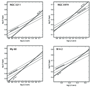
Figure 7: The solution to the absolute luminosity and distance of the PNe given by the requirement that both the reddening-corrected observed H$\beta$ flux and the observed angular size of the PNe agree with those predicted by the photoionisation model. The error bands are the measurement errors of the observed quantities.

6.2 Location of CSs on the H-R Diagram

With a reasonably accurate knowledge of the distance, we can now place the central stars on the Hertzsprung-Russell (H-R) Diagram. For this purpose, we adopt a mean of the statistical and photoinisation distances: NGC 3211 $3.2^{+1.2}_{-1.0}$ kpc; NGC 5979 $2.7^{+1.0}_{-0.7}$ kpc; My 60 $3.9^{+1.1}_{-0.8}$ kpc; M 4-2 $5.8^{+1.7}_{-1.5}$ kpc. With these distances, we derive stellar luminosities and their errors, and from the models, we also provide the derived stellar temperatures with their estimated measurement errors. These are given in Table 8.

Table 8: Derived Central star parameters.

	log L ($L_{\odot}$)	log $T_{\rm eff}$ K
NGC 3211	$3.30^{+0.13}_{-0.13}$	$5.16^{+0.03}_{-0.03}$
NGC 5979	$3.18^{+0.15}_{-0.15}$	$5.20^{+0.03}_{-0.03}$
My 60	$3.39^{+0.17}_{-0.17}$	$5.11^{+0.03}_{-0.03}$
M 4-2	$3.44^{+0.20}_{-0.18}$	$5.13^{+0.03}_{-0.03}$

In Figure 8 we locate these stars on the Hertzprung-Russell diagram. Overlaid are the H-burning $Z=0.016$ tracks from Vassiliadis & Wood (1994). What is remarkable is the manner in which the four objects of our study cluster tightly together, suggesting very similar precursor stars. All are consistent with having initial masses between 1.5 and 2.0 M_⊙, and having an evolutionary age of about 6000 yr. It is interesting that the only bona-fide double-shell PN, NGC 5979, seems to have the highest mass precursor. This would be consistent with the evolutionary scenario of Vassiliadis & Wood (1993), in that the He-shell flashes occur more frequently in higher mass precursors, driving “super-wind” episodes which then form multiple shells in the subsequent PNe.

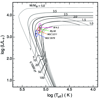
Figure 8: The location of our PNe on the (hydrogen-burning) H-R diagram as derived from photoionisation modelling compared with evolutionary tracks of central stars of PNe from Vassiliadis & Wood (1994). The four objects are remarkably similar, and consistent with having initial masses in the range $1.5-2.0{\rm M}_{\odot}$, and evolutionary ages of about 6000yr.

The age of the PNe as measured from the H-burning tracks is in fact the time since the central star became hotter than $10^{4}$K. This can be directly compared to the estimated dynamical ages given from the diameters given above, and the expansion velocity in the low-ionisation species as given in Table 6. These are respectively; NGC 3211 $\tau_{\rm dyn}=3000$yr, NGC 5979 $\tau_{\rm dyn}=3950$yr, My 60 $\tau_{\rm dyn}=3100$yr, and M 4-2 $\tau_{\rm dyn}=4500$yr. The dynamical ages are somewhat shorter than the age implied from the evolutionary tracks, but both methods agree that the ages of these four PNe are very similar. Due to acceleration or deceleration of the nebular shell, driven by the changing stellar wind parameters during its dynamical evolution, we have no reason to expect that the dynamical age derived will be exactly equal to the age inferred by the position of the PN on the evolutionary track. Thus we see no serious discrepancy between the dynamical and the evolutionary age. If we were to use the recent models of Miller Bertolami (2015), then the observed dynamical ages would show closer agreement to the theoretical ages derived from the position of PNe along the post-AGB track.

7 Conclusions

In this paper we have studied four PNe, three of which had been classified with central stars of the WELS type, and the fourth which showed the same set of recombination lines of highly-excited ions which are thought to characterise a WELS; C IV at 5801-12Å and the N III, C III, and C IV complex feature at 4650Å. We have, however, demonstrated that these emission lines arise not in the central star, but are instead distributed throughout the nebular gas. We find no trace of these emission originating from the central stars themselves. Instead, we identify O VI $\lambda\lambda 3811.3,3834.2$ in three of the central stars, and in the case of NGC 5979 the O V $\lambda 4664.4$ line as well. Thus, at least three of the central stars are not WELS, but are in fact hot O(H) stars. This result casts doubt on the reality of the WELS class as a whole, a result made possible only by the fact that we have integral field spectroscopy covering the whole nebula.

We cannot use nebular emission line characteristics to define a class of the central star, since the nebular lines depend on the nature of the EUV spectrum, the chemical abundances, the density and the geometry of the gas with respect to the central star. We always define the central star type itself from the UV, visible or IR emissions of the central star. If the emission lines which have been used to classify the star instead arise in the nebula, as we have demonstrated here in four independent examples, then the classification has no validity. Clearly, as in the case of binary systems, some real examples of WELS exist. However, given that we have found four out of four examples of misclassification, we believe that many other cases of such misclassification may exist. This is the major conclusion of this paper.

As to why the C IV at 5801-12 Å and the N III, C III, and C IV complex feature at 4650 Å are so strong, we cannot provide a solution, since we do not have the required atomic data relating to the effective recombination coefficients. It may be possible that we have C and N- rich pockets of gas in the nebula, but then why would these species be distributed in exactly the way we would expect in terms of the local excitation? Figures 1 and 3 are remarkably similar.

Apart from the standard nebular analysis techniques used to probe chemical abundances and physical conditions in the nebula, we have been able to apply self-consistent photoionisation modelling to an analysis of the integrated spectrum of these PNe. We find that an optically-thin isobaric model with an inner empty zone and, in some cases, an additional optically-thick zone provides an excellent description of the observed spectrum, and provides a good estimate of the stellar effective temperature. Generally speaking, the agreement between the two analysis methods is quite satisfactory as far as the abundance determinations are concerned.

According to the derived chemical abundances from the NEAT, none of our objects was classified as Type I PN. We find that the chemical compositions of both NGC 3211 and NGC 5979 are consistent with being of Type IIa, while that of My 60 and M 4-2 are consistent with the Type IIb/III classification. Considering also their calculated Galactic vertical heights and peculiar velocities, we suggest that NGC 3211 is probably a member of the Galactic thin disk, while both My 60 and M 4-2 are Galactic thick members.

Additionally, the self consistent modelling yields a number of additional parameters. Specifically, we are able to use the models to provide a new “Strömgren Distance” estimate, which agrees - within the errors - with the distances derived from the standard statistical techniques. We find that all four PNe are highly-excited nebulae optically-thin to the escape of EUV photons. With a knowledge of the distance, another parameters derived from the models, we are also able to constrain the luminosity of the central star, placing it on the H-R Diagram.

All four PNe studied in this paper are of remarkably similar $T_{\rm eff}$ and luminosity, are at a very similar evolutionary stage with ages in the range 3000-6000 yr, and are all derived from precursor stars in the restricted mass range $1.5-2.0$ M_⊙.

Appendix A Measured Emission Line Fluxes

We determined the final integrated emission-line fluxes from the combined, flux-calibrated blue and red spectra of each PN. The line fluxes and their measurement uncertainties were determined using the IRAF splot task and were integrated between two given limits, over a local continuum fitted by eye, using multiple Gaussian fitting for the line profile.

The amount of interstellar reddening was determined by the NEAT code from the ratios of hydrogen Balmer lines, in an iterative method. Firstly, the reddening coefficient, $c(H\beta)$, was calculated assuming intrinsic $H\alpha$, $H\beta$, $H\gamma$ line ratios for a temperature ($T_{e}$) of 10000K and density ($N_{e}$) of 1000 cm^-3, which were used to de-reddened using this value the line list. Secondly, the electron temperature and density were calculated as explained in section (3.2). After that, the intrinsic Balmer line ratios were re-calculated at the convenient temperature and density, and again $c(H\beta)$ was recalculated. The line intensities have been corrected for extinction by adopting the extinction law of Howarth (1983). The estimated reddening coefficients and observed $H\beta$ fluxes of the sample are listed in Table 2, while Table 9 lists the observed and de-reddened line strengths of the sample. Columns (1) & (2) give the laboratory wavelengths and identification of observed emission lines, while columns (3)-(10) give the observed F($\lambda$) and the de-reddened line strengths I($\lambda$), scaled to $H\beta=100$. A total of $\sim$ 128 distinct emission lines were identified in each nebula, which include $\sim$ 88 permitted and 40 forbidden lines.

Table 9: Line fluxes and de-reddened intensities, relative to H$\beta=100$, of NGC 3211, NGC 5979, My 60, and M 4-2. The full version of the table is available online. A portion is shown here for guiding the reader regarding its content.

		NGC 3211		NGC 5979		My 60		M 4-2
Lab (Å)	ID	F($\lambda$)	I($\lambda$)	F($\lambda$)	I($\lambda$)	F($\lambda$)	I($\lambda$)	F($\lambda$)	I($\lambda$)
3868.76	[Ne III]	92.5$\pm$1.85	112.4$\pm$4.1	47.1$\pm$1.41	58.4$\pm$3.12	57.2$\pm$1.72	90.3$\pm$4.96	48.1$\pm$0.96	65.3$\pm$2.34
3889.06	HI 8-2	13.6$\pm$0.27	16.4$\pm$0.60	9.3$\pm$0.28	11.5 $\pm$0.62	10.1$\pm$0.30	15.8$\pm$0.85	10.7$\pm$0.21	14.5 $\pm$0.52
3923.48	He II	0.4$\pm$0.04	0.5$\pm$0.05	0.6$\pm$0.02	0.8$\pm$0.04			0.5$\pm$0.01	0.7$\pm$0.03
3967.47	[Ne III]	30.6$\pm$0.61	36.5$\pm$1.30	14.4 $\pm$0.43	17.5 $\pm$0.91	15.1$\pm$0.45	22.9$\pm$1.24	12.0$\pm$0.24	15.9 $\pm$0.56
3970.08	HI 7-2	13.2$\pm$0.26	15.8$\pm$0.56	11.8 $\pm$0.35	14.3 $\pm$0.75	10.1$\pm$0.30	15.3$\pm$0.80	11.8$\pm$0.24	15.5 $\pm$0.54
4025.61	He II							1.5$\pm$0.05	2.0$\pm$0.08
4026.08	N II	1.5$\pm$0.15	1.8$\pm$0.19	1.3$\pm$0.04	1.5$\pm$0.08	1.3$\pm$0.13	1.9$\pm$0.21
4068.60	[S II]	1.5$\pm$0.08	1.8$\pm$0.10	1.1$\pm$0.03	1.3$\pm$0.07	1.4$\pm$0.10	2.0$\pm$0.16	1.9$\pm$0.06	2.4$\pm$0.10

References

- Acker & Neiner (2003) Acker A., Neiner C., 2003, A&A, 403, 659
- Acker et al. (1991) Acker A., Raytchev B., Stenholm B., Tylenda R., 1991, A&AS, 90, 89
- Ali et al. (2015a) Ali A., Ismail H. A., Alsolami Z., 2015a, Ap&SS, 357, 21
- Ali et al. (2015b) Ali A., Amer M. A., Dopita M. A., Vogt F. P. A., Basurah H. M., 2015b, A&A, 583, A83
- Aller (1956) Aller L. H., 1956, Gaseous nebulae. London: Chapman & Hall, 1956
- Baessgen & Grewing (1989) Baessgen M., Grewing M., 1989, A&A, 218, 273
- Balick et al. (1993) Balick B., Rugers M., Terzian Y., Chengalur J. N., 1993, ApJ, 411, 778
- Balick et al. (1994) Balick B., Perinotto M., Maccioni A., Terzian Y., Hajian A., 1994, ApJ, 424, 800
- Balick et al. (1998) Balick B., Alexander J., Hajian A. R., Terzian Y., Perinotto M., Patriarchi P., 1998, AJ, 116, 360
- Campbell & Moore (1918) Campbell W. W., Moore J. H., 1918, Publications of Lick Observatory, 13, 75
- Childress et al. (2014) Childress M. J., Vogt F. P. A., Nielsen J., Sharp R. G., 2014, Ap&SS, 349, 617
- Corradi et al. (2003) Corradi R. L. M., Schönberner D., Steffen M., Perinotto M., 2003, MNRAS, 340, 417
- Corradi et al. (2007) Corradi R. L. M., Steffen M., Schönberner D., Jacob R., 2007, A&A, 474, 529
- Corradi et al. (2011) Corradi R. L. M., et al., 2011, MNRAS, 410, 1349
- Crowther et al. (1998) Crowther P. A., De Marco O., Barlow M. J., 1998, MNRAS, 296, 367
- Danehkar & Parker (2015) Danehkar A., Parker Q. A., 2015, MNRAS, 449, L56
- Danehkar et al. (2013) Danehkar A., Parker Q. A., Ercolano B., 2013, MNRAS, 434, 1513
- Danehkar et al. (2014) Danehkar A., Todt H., Ercolano B., Kniazev A. Y., 2014, MNRAS, 439, 3605
- Dopita (1997) Dopita M. A., 1997, ApJ, 485, L41
- Dopita & Sutherland (2000) Dopita M. A., Sutherland R. S., 2000, ApJ, 539, 742
- Dopita et al. (2007) Dopita M., Hart J., McGregor P., Oates P., Bloxham G., Jones D., 2007, Ap&SS, 310, 255
- Dopita et al. (2010) Dopita M., et al., 2010, Ap&SS, 327, 245
- Dopita et al. (2013) Dopita M. A., Sutherland R. S., Nicholls D. C., Kewley L. J., Vogt F. P. A., 2013, ApJS, 208, 10
- Durand et al. (1998) Durand S., Acker A., Zijlstra A., 1998, A&AS, 132, 13
- Fogel et al. (2003) Fogel J., De Marco O., Jacoby G., 2003, in Kwok S., Dopita M., Sutherland R., eds, IAU Symposium Vol. 209, Planetary Nebulae: Their Evolution and Role in the Universe. p. 235
- Frew & Parker (2010) Frew D. J., Parker Q. A., 2010, Publ. Astron. Soc. Australia, 27, 129
- Frew & Parker (2012) Frew D. J., Parker Q. A., 2012, in IAU Symposium. pp 192–195, arXiv:1203.1388, doi:10.1017/S1743921312010940
- Frew et al. (2016) Frew D. J., Parker Q. A., Bojičić I. S., 2016, MNRAS, 455, 1459
- Gathier & Pottasch (1989) Gathier R., Pottasch S. R., 1989, A&A, 209, 369
- Gathier et al. (1986) Gathier R., Pottasch S. R., Pel J. W., 1986, A&A, 157, 171
- Gieseking et al. (1986) Gieseking F., Hippelein H., Weinberger R., 1986, A&A, 156, 101
- Girard et al. (2007) Girard P., Köppen J., Acker A., 2007, A&A, 463, 265
- Górny (2014) Górny S. K., 2014, A&A, 570, A26
- Górny et al. (1999) Górny S. K., Schwarz H. E., Corradi R. L. M., Van Winckel H., 1999, A&AS, 136, 145
- Grevesse et al. (2010) Grevesse N., Asplund M., Sauval A. J., Scott P., 2010, Ap&SS, 328, 179
- Gruenwald & Viegas (1995) Gruenwald R., Viegas S. M., 1995, A&A, 303, 535
- Gurzadian (1988) Gurzadian G. A., 1988, Ap&SS, 149, 343
- Hajduk et al. (2010) Hajduk M., Zijlstra A. A., Gesicki K., 2010, MNRAS, 406, 626
- Hajian et al. (1997) Hajian A. R., Balick B., Terzian Y., Perinotto M., 1997, ApJ, 487, 304
- Hajian et al. (2007) Hajian A. R., et al., 2007, ApJS, 169, 289
- Henry et al. (2004) Henry R. B. C., Kwitter K. B., Balick B., 2004, AJ, 127, 2284
- Jenkins (2009) Jenkins E. B., 2009, ApJ, 700, 1299
- Kaler et al. (1996) Kaler J. B., Kwitter K. B., Shaw R. A., Browning L., 1996, PASP, 108, 980
- Kingsburgh & Barlow (1994) Kingsburgh R. L., Barlow M. J., 1994, MNRAS, 271, 257
- Liu & Danziger (1993) Liu X.-W., Danziger J., 1993, MNRAS, 263, 256
- Lodders et al. (2009) Lodders K., Palme H., Gail H.-P., 2009, Landolt Börnstein, p. 44
- Maciel & Quireza (1999) Maciel W. J., Quireza C., 1999, A&A, 345, 629
- Marcolino & de Araújo (2003) Marcolino W. L. F., de Araújo F. X., 2003, AJ, 126, 887
- Marcolino et al. (2007) Marcolino W. L. F., de Araújo F. X., Junior H. B. M., Duarte E. S., 2007, AJ, 134, 1380
- Mathewson et al. (2013) Mathewson D. S., Hart J., Wehner H. P., Hovey G. R., van Harmelen J., 2013, Journal of Astronomical History and Heritage, 16, 2
- Mathis et al. (1977) Mathis J. S., Rumpl W., Nordsieck K. H., 1977, ApJ, 217, 425
- Meatheringham & Dopita (1991) Meatheringham S. J., Dopita M. A., 1991, ApJS, 75, 407
- Meatheringham et al. (1988) Meatheringham S. J., Wood P. R., Faulkner D. J., 1988, ApJ, 334, 862
- Mendez (1991) Mendez R. H., 1991, in Michaud G., Tutukov A. V., eds, IAU Symposium Vol. 145, Evolution of Stars: the Photospheric Abundance Connection. p. 375
- Milingo et al. (2002) Milingo J. B., Henry R. B. C., Kwitter K. B., 2002, ApJS, 138, 285
- Miller Bertolami (2015) Miller Bertolami M. M., 2015, ArXiv e-prints,
- Miszalski (2009) Miszalski B., 2009, PhD thesis, Department of Physics, Macquarie University, NSW 2109, Australia
- Miszalski et al. (2011) Miszalski B., Corradi R. L. M., Boffin H. M. J., Jones D., Sabin L., Santander-García M., Rodríguez-Gil P., Rubio-Díez M. M., 2011, MNRAS, 413, 1264
- Monreal-Ibero et al. (2005) Monreal-Ibero A., Roth M. M., Schönberner D., Steffen M., Böhm P., 2005, ApJ, 628, L139
- Monteiro et al. (2013) Monteiro H., Gonçalves D. R., Leal-Ferreira M. L., Corradi R. L. M., 2013, A&A, 560, A102
- Nieva & Przybilla (2012) Nieva M.-F., Przybilla N., 2012, A&A, 539, A143
- Parthasarathy et al. (1998) Parthasarathy M., Acker A., Stenholm B., 1998, A&A, 329, L9
- Peimbert (1978) Peimbert M., 1978, in Terzian Y., ed., IAU Symposium Vol. 76, Planetary Nebulae. pp 215–223
- Peimbert & Torres-Peimbert (1983) Peimbert M., Torres-Peimbert S., 1983, in Flower D. R., ed., IAU Symposium Vol. 103, Planetary Nebulae. pp 233–241
- Peimbert & Torres-Peimbert (1987) Peimbert M., Torres-Peimbert S., 1987, Rev. Mex. Astron. Astrofis., 14, 540
- Perinotto (1991) Perinotto M., 1991, ApJS, 76, 687
- Phillips (2000) Phillips J. P., 2000, AJ, 119, 2332
- Quireza et al. (2007) Quireza C., Rocha-Pinto H. J., Maciel W. J., 2007, A&A, 475, 217
- Rauch (2003) Rauch T., 2003, A&A, 403, 709
- Reid & Parker (2010) Reid W. A., Parker Q. A., 2010, Publ. Astron. Soc. Australia, 27, 187
- Ruffle et al. (2004) Ruffle P. M. E., Zijlstra A. A., Walsh J. R., Gray M. D., Gesicki K., Minniti D., Comeron F., 2004, MNRAS, 353, 796
- Schneider & Terzian (1983) Schneider S. E., Terzian Y., 1983, ApJ, 274, L61
- Schönberner et al. (2005) Schönberner D., Jacob R., Steffen M., 2005, A&A, 441, 573
- Schwarz et al. (1992) Schwarz H. E., Corradi R. L. M., Melnick J., 1992, A&AS, 96, 23
- Scott et al. (2015a) Scott P., et al., 2015a, A&A, 573, A25
- Scott et al. (2015b) Scott P., Asplund M., Grevesse N., Bergemann M., Sauval A. J., 2015b, A&A, 573, A26
- Shaw & Kaler (1989) Shaw R. A., Kaler J. B., 1989, ApJS, 69, 495
- Stanghellini et al. (1993) Stanghellini L., Corradi R. L. M., Schwarz H. E., 1993, A&A, 279, 521
- Stanghellini et al. (2002) Stanghellini L., Shaw R. A., Mutchler M., Palen S., Balick B., Blades J. C., 2002, ApJ, 575, 178
- Surendiranath & Pottasch (2008) Surendiranath R., Pottasch S. R., 2008, A&A, 483, 519
- Tsamis et al. (2007) Tsamis Y. G., Walsh J. R., Pequignot D., Barlow M. J., Liu X.-W., Danziger I. J., 2007, The Messenger, 127, 53
- Tylenda et al. (1992) Tylenda R., Acker A., Stenholm B., Koeppen J., 1992, A&AS, 95, 337
- Tylenda et al. (1993) Tylenda R., Acker A., Stenholm B., 1993, A&AS, 102, 595
- Vassiliadis & Wood (1993) Vassiliadis E., Wood P. R., 1993, ApJ, 413, 641
- Vassiliadis & Wood (1994) Vassiliadis E., Wood P. R., 1994, ApJS, 92, 125
- Wang et al. (2004) Wang W., Liu X.-W., Zhang Y., Barlow M. J., 2004, A&A, 427, 873
- Weidmann & Gamen (2011) Weidmann W. A., Gamen R., 2011, A&A, 526, A6
- Weidmann et al. (2015) Weidmann W. A., Méndez R. H., Gamen R., 2015, A&A, 579, A86
- Zhang (1993) Zhang C. Y., 1993, ApJ, 410, 239
- Zhang & Kwok (1993) Zhang C. Y., Kwok S., 1993, ApJS, 88, 137