Patch-Ordering as a Regularization for Inverse Problems in Image Processing

Abstract

Recent work in image processing suggests that operating on (overlapping) patches in an image may lead to state-of-the-art results. This has been demonstrated for a variety of problems including denoising, inpainting, deblurring, and super-resolution. The work reported in [1, 2] takes an extra step forward by showing that ordering these patches to form an approximate shortest path can be leveraged for better processing. The core idea is to apply a simple filter on the resulting 1D smoothed signal obtained after the patch-permutation. This idea has been also explored in combination with a wavelet pyramid, leading eventually to a sophisticated and highly effective regularizer for inverse problems in imaging.

In this work we further study the patch-permutation concept, and harness it to propose a new simple yet effective regularization for image restoration problems. Our approach builds on the classic Maximum A’posteriori probability (MAP), with a penalty function consisting of a regular log-likelihood term and a novel permutation-based regularization term. Using a plain 1D Laplacian, the proposed regularization forces robust smoothness ($L1$) on the permuted pixels. Since the permutation originates from patch-ordering, we propose to accumulate the smoothness terms over all the patches’ pixels. Furthermore, we take into account the found distances between adjacent patches in the ordering, by weighting the Laplacian outcome.

We demonstrate the proposed scheme on a diverse set of problems: (i) severe Poisson image denoising, (ii) Gaussian image denoising, (iii) image deblurring, and (iv) single image super-resolution. In all these cases, we use recent methods that handle these problems as initialization to our scheme. This is followed by an L-BFGS optimization of the above-described penalty function, leading to state-of-the-art results, and especially so for highly ill-posed cases.

1 Introduction

In recent years we see an interesting trend, in which many image restoration algorithms choose to operate on local image patches rather than processing the image as a whole. These techniques impose statistical prior knowledge on the patches of the processed image. Surprisingly, in many cases these methods lead to state-of-the-art results. For example, in the Gaussian denoising case, the algorithm presented in [3] performs denoising using a statistical model based on sparse representation of the image patches, training a dictionary using the K-SVD algorithm. The BM3D algorithm reported in [4] exploits interrelations between patches by grouping them into 3D groups, and applying collaborative filtering on them that is based on sparse representation as well. The work reported in [5, 6, 7] extends PCA and dictionary learning, both in the context of patches for handling severe Poisson image denoising. The scheme reported in [8] adopts the sparse representation model to handle the single image super-resolution problem. The papers [9, 10] both propose a GMM modeling of image patches, and demonstrate the effectiveness of this to variety of inverse problems. The NSCR method by Dong et. al. [11] uses sparse representation for solving both the super-resolution and the deblurring problems. The IDD-BM3D method in [12] employs BM3D frames for image deblurring. All these papers and many others rely on operating on patches in order to complete the restoration task at hand. Many works use sophisticated priors when operating locally, and most often they resort to a simple averaging when combining the restored patches.

The work reported in [1] takes another step toward exploiting interrelations between image patches in the image. The work reported in [1] proposes to construct a 1D smoothed signal by applying a permutation on the pixels of the corrupted image. The permutation is obtained by ordering image patches to form ”the shortest possible path”, approximating the solution of the traveling salesman problem (TSP). Given the sorted image, the clean image is recovered by applying a 1D filter on the ordered signal. This method is simple and yet it leads to high-quality results. On the down side, it is limited to the Gaussian denoising and inpainting problems. The work reported in [2] takes an extra step in exploring the patch-ordering concept. This work constructs a sophisticated and very powerful regularizer by combining the patch-permutation idea with a wavelet pyramid [13, 14]. The obtained regularizer is used for solving general inverse problems in imaging. This method leads to high-quality results in series of tests, however it is quite involved.

In this paper we propose to compose the whole image from local patches using a prior that exploits interrelation between them. We harness the patch-permutation idea, merging it with the classical Maximum A’posteriori probability (MAP) estimator, by proposing a new, simple, yet powerful regularization for inverse imaging problems. We formulate the inverse problem as a weighted sum of two penalty terms: (i) a regular negative log-likelihood, and (ii) a novel regularization expression that forces smoothness in a robust way, by basing it on reordered list of the image pixels, obtained according to the similarity of image patches.

For constructing the permutation-based regulatization, we follow the core idea presented in [1]. We rely on the assumption that in an ideal image, close similarity between patches indicates a proximity between their center pixels. We therefore build a 1D (piece-wise) smoothed signal by applying a patch-based permutation on the restored (unknown) image pixels. The permutation is obtained by extracting all possible patches with overlaps from the currently recovered image, and ordering them to form the (approximated) shortest possible path. The resulting ordering induces the permutation.

The proposed regularization forces smoothness on the obtained 1D signal via a Laplacian, penalized by the robust ${L_{1}}$ norm. Since the ordering is associated with all the pixels withing the patches, the smoothness term is accumulated over all these pixels. We also deploy weights that take into account the actual distances between the consecutive patches in the ordering.

The proposed scheme is demonstrated on several different problems: (i) White additive Gaussian image denoising, (ii) severe Poisson image denoising, (iii) image deblurring, and (iv) single image super-resolution. We initialize our algorithm with an output of a recent method that handles each of these problems. The reconstructed image is then obtained by minimizing the penalty function described above using the L-BFGS method [15, 16]. Our extensive experiments indicate that applying the proposed scheme leads to state-of-the-art results.

We should note that the proposed scheme bares some similarity to recent work offering regularization of inverse problems by utilizing the similarity between patches formed as a graph [17, 18, 19, 20, 21, 22, 23, 24, 25]. These works propose various formats of using this graph’s Laplacian as a sparsifying operator. Our approach could be considered as a special case of such a Laplacian regularization, which forces the graph to be a simple and continuous chained ordering of the image pixels. As such, the regularization we obtain is simpler and easier to manage (since we keep only one forward and one backward neighbors per each pixel). In addition, our approach also provides a stronger stabilizing effect for highly ill-posed problems since it ties all the pixels to each other.

The paper is organized as follows. In Section 2 we discuss the principles behind the permutation construction, and how it becomes useful as a regularizer. Section 3 describes the proposed algorithm, along with the numerical scheme used. Section 4 presents experiment results and compares the new method with other leading schemes. Section 6 concludes this paper and raises directions for a future work.

2 Constructing the permutation

A common assumption in image processing is that clean images are usually (piece-wise) smooth, i.e. the difference between any two neighboring pixels tends to be small. Most image processing algorithms, be it for restoration, segmentation, compression, and more, rely on this model to some extent. The problem with this assumption, however, is that violation from this behavior is due to image edges and texture, and both are central in forming and defining the visual content of an image, and as such, they cannot be sacrificed as simple outliers.

Adopting a totally different perspective towards handling of an image, a convenient and often used technique for developing an image processing algorithm is to convert the 2D image into a 1D array, treat the image as a vector, and then convert the resulting 1D array back to a 2D array. There are several popular scan methods that convert an image to a vector, the prominent of which are raster scan, zigzag scan, Hilbert Peano and other space-filling curves.

The question we pose now is this: how can we combine the two approaches mentioned above? Namely, given a corrupted image ${\mathbf{y}\in\mathbb{R}^{N}}$, how should we construct a 2D-to-1D conversion that produces the smoothest possible vector when applied to a clean image, ${\mathbf{x}}$. Such a conversion would be extremely helpful for image restoration tasks, because in the 1D domain its processing is expected to be very simple and effective. We should emphasize that the sought conversion method must be robust, i.e. be able to produce a meaningful ordering even when operated on a corrupted data.

A word on notations: The 2D-to-1D conversion we are seeking is denoted by ${\Omega}$, and represented by a permutation matrix ${P}$. I.e., applying ${P}$ to column-stacked image ${\mathbf{x}}$, ${P\mathbf{x}}$, produces a vector with the reordering ${\Omega}$.

In this work we build on the ideas presented in [1], while giving it a new and novel interpretation. In order to propose such a smoothing conversion, we shall assume that each pixel of the clean image ${\mathbf{x}}$ can be represented by the corresponding surrounding patch taken from the corrupted image ${\mathbf{y}}$. In other words, the assumption is that if two patches of the corrupted (or clean) image are close in terms of some distance function, then their corresponding central pixels in the clean image are expected to be similar as well. We will refer hereafter to this as the $A1$ assumption. Throughout this work we shall use the Euclidean distance for assessing proximity between patches. We extract all possible patches ${\{\mathbf{z_{i}}\}_{1}^{N}}$ of size ${\sqrt{n}\times\sqrt{n}}$ with overlaps from the image ${\mathbf{y}}$, where ${n\ll N}$. Our method refers to the patches as points in ${\mathbb{R}^{n}}$, defining a graph where the patches are its vertices and distances between them are the edges.

Recall that our aim is to find an ordering ${\Omega}$ (or ${P}$, its permutation matrix equivalent) such that the resulting permuted clean image is the smoothest. This can be defined as the following minimization task:

$$\min_{P}\|DP\mathbf{x}\|_{1}=\min_{\Omega}\sum_{i=2}^{N}\left|x_{\Omega(i)}-x_{\Omega(i-1)}\right|\;,$$ (1)

where ${D}$ is a 1D difference operator (simple derivative). Interestingly, it is tempting to propose an ordering of the image patches in ${\mathbf{x}}$ based on a simple sort of their center pixels, as it will lead to the ideal (smoothest) permutation. However, since we assume that ${\mathbf{x}}$ is not available and instead we have ${\mathbf{y}}$, this option is impossible. Thus, the above objective is replaced by an alternative that relies on the assumption ${A1}$ made above:

$$\min_{P}\|DP\mathbf{x}\|_{1}\approx\min_{\Omega}\sum_{i=2}^{N}\left\|\mathbf{z}_{\Omega(i)}-\mathbf{z}_{\Omega(i-1)}\right\|_{2}\;.$$ (2)

This means that the graph vertices are ordered to form the shortest possible path that visits each vertex exactly once. Namely, we formulate the quest of $\Omega$ as a classic Traveling Salesman Problem (TSP) [26].

A natural way to proceed is to use a known approximation algorithm that is known to perform well for the TSP. The problem with this approach is that the permutation induced from a too-good TSP solver is in fact creating and magnifying artifacts. An example for this behavior and the artifacts induced are shown in Figure 1, where we use the Lin-Kernighan algorithm for approximating the TSP solution [27, 28], and then apply our recovery algorithm. We should note that the two orderings (our approach, as described in Algorithm LABEL:alg:reordering and Lin-Kernighan) lead to an average total variation measure, $\sum_{k=1}^{N-1}|\mathbf{x}_{k+1}-\mathbf{x}_{k}|$, of $2.17\times 10^{-2}$ and $1.79\times 10^{-2}$, respectively, when assessed on the original (true) image. This implies that the better ordering leads to $17.5$% improvement in terms of the smoothness obtained, but this does not translate to better outcome in our algorithm.

The problem with a too-good TSP solver is that it adjusts the ordering to artifacts in the initial image, thereby creating correlation between the regularizer and the artifacts, which magnifies these artifacts.

(a) The initial image (BM3D)
PSNR = 25.87dB

(b) Output with Lin-Kernighan
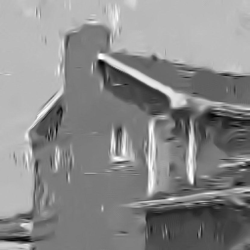
PSNR = 24.17dB

(c) Output with Algorithm LABEL:alg:reordering
PSNR = 26.63dB

Fig. 1: The output of our scheme with Lin-Kernighan heuristics or Algorithm LABEL:alg:reordering for solving the TSP problem. The scheme is applied for the Gaussian denoising task with ${\sigma=100}$, and initialized with the BM3D result.

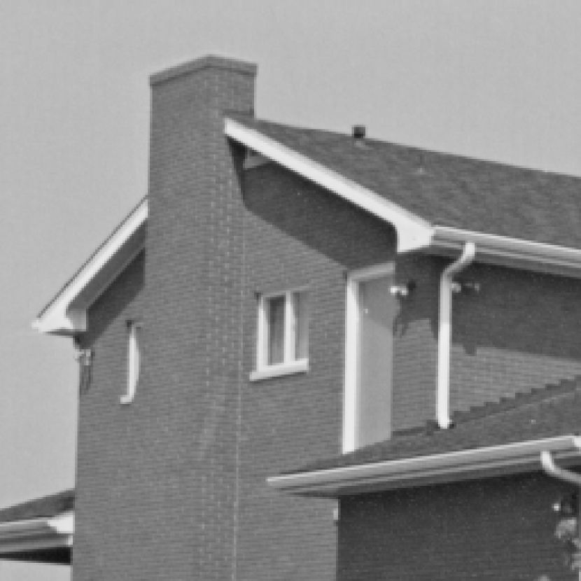
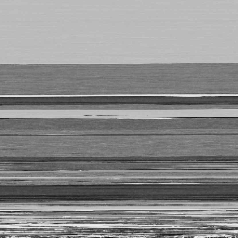
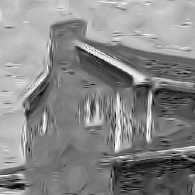
In order to overcome this artifact magnification problem we use a randomized approach for the TSP solution. More specifically, we use the randomized version of NN (Nearest Neighbor) heuristics presented in [1] as a TSP solver. This algorithm starts from an arbitrary patch ${\mathbf{z}_{i_{0}}}$ and continues by finding the closest two neighbors to the currently held vertex with the restriction that they have not been assigned yet, choosing one of them at random. At the $k$-th stage of the algorithm we have accumulated already $k$ vertices. Given the last of them, ${\mathbf{z}_{\Omega(k)}}$, we choose either ${\mathbf{z}_{i1}}$ or ${\mathbf{z}_{i2}}$, its two closest neighbors, with probabilities ${p_{1}=\alpha\cdot\exp{\left(-\|\mathbf{z}_{\Omega(k)}-\mathbf{z}_{i_{1}}\|_{2}^{2}/\delta\right)}}$ and ${p_{2}=\alpha\cdot\exp{\left(-\|\mathbf{z}_{\Omega(k)}-\mathbf{z}_{i_{2}}\|_{2}^{2}/\delta\right)}}$, where ${\alpha}$ is chosen such as ${p_{1}+p_{2}=1}$. The nearest neighbor search is performed from within the set of unvisited patches, and it is limited to a window of size ${B\times B}$ around $\mathbf{z}_{\Omega{k}}$. If there is only one unvisited patch in this region, the heuristics chooses it. When no unvisited patches remain, the first and second nearest neighbor search is performed among all unvisited image patches. The ${B\times B}$ square restriction is designed to reduce computation complexity; however it is important also for assuring that relevant patches are matched. The randomized NN heuristics is summarized in Algorithm LABEL:alg:reordering. An example of a reordered image is presented in Figure 2.

A drawback of the described reordering is it’s greediness nature. Indeed, as can be seen in Figure 2, the last part of the reordered clean image is not smooth. This is due to the fact that in the last stages of Algorithm LABEL:alg:reordering very few unvisited patches remain for the nearest neighbor search. While this may seem troubling, in section 5 we shall explain why this phenomenon has little effect on the final restored results.

(a) Original image

(b) Reordered image

Fig. 2: The original and the reordered House image. Notice that the last portion of the reordered image is not smooth, due to the greedy nature of the NN heuristics in Algorithm LABEL:alg:reordering.

3 The reconstruction algorithm

3.1 Constructing the Regularization Term

Our regularizer is constructed as a sum of several smoothness terms. A smoothness term is obtained by applying the matrices $P$, $L$ and $M$ to the column-stacked image $\mathbf{x}$, ${MLP\mathbf{x}}$, and penalizing the result by the robust $L_{1}$ norm:

$$r(\mathbf{x})=\|MLP\mathbf{x}\|_{1}\;.$$ (3)

In this expression ${P}$ is the permutation matrix that represents the ordering $\Omega$ obtained by the TSP solver. ${L}$ is a simple 1D Laplacian, and ${M}$ is a weighting diagonal matrix of the form ${M=diag(m_{k})}$, where

$$m_{k}=\min\{\frac{\gamma_{k}}{\beta_{k}},m_{max}\}\;.$$ (4)

The weights $\{m_{k}\}_{1}^{N}$ take into account the distances between the consecutive patches in the ordering. Intuitively we expect that the centers of the closer patches will be more similar. Therefore the weights are chosen to be inversely proportional to the ${L_{2}}$ norm of the 1D-Laplacian of the corresponding patches. In other words, the ${\beta_{k}}$ coefficients are calculated using the following formula:

$$\beta_{k}=\frac{1}{2}\left\|2\mathbf{z}_{k}-\mathbf{z}_{k-1}-\mathbf{z}_{k+1}\right\|_{2}\;,$$ (5)

where ${1\leq{k}\leq{N}}$, and $\{\mathbf{z}_{k}\}_{1}^{N}$ are the ordered patches. The boundary cases ($k=1$, and $k=N$) are handled by setting ${\mathbf{z}_{0}=\mathbf{z}_{1}}$, and ${\mathbf{z}_{N+1}=\mathbf{z}_{N}}$. We note that if $\beta_{k}$ would have been defined as in Equation (5), but assuming patches of size $1\times 1$ pixels (i.e., only the center pixel is the actual patch), then our regularization simplifies to become the $L_{0}$-norm. The reason is that in this case $\beta_{k}$ hold simply the absolute values of the 1D Laplacian over the ordered pixels. The penalty term itself computes the very same Laplacian and divides by these $\beta_{k}$ values. Thus, all those ratios are ’1’-es for non-zero values and ’0’ elsewhere, thus obtaining an $L_{0}$-norm. Thus, the term $r(\mathbf{x})$ in Equation (3) seeks to sparsify the second derivative of the permuted image in a robust way.

The problem with the $\{1/\beta_{k}\}_{1}^{N}$ coefficients is that the distances between the patches which contain edges or texture are usually relatively high, and therefore these weights are relatively low. The coefficients ${\{\gamma_{k}\}_{1}^{N}}$ that appear in Equation (4) are designed to overcome this problem, by magnifying the weights for edge/texture patches,

$$\gamma_{k}=\begin{cases}\gamma_{edge}&\text{patch }\mathbf{z}_{k}\text{ contains edges,}\\ 1&\mathbf{z}_{k}\text{ is a flat patch,}\end{cases}$$ (6)

where $\gamma_{edge}\geq 1$ is a parameter to be set. In order to identify patches that contain edges or texture, our algorithm calculates the magnitude of image gradient using the central difference method. Namely, ${g_{i,j}}$, the magnitude of the gradient at location ($i$, $j$), is calculated using:

$$g_{i,j}=\sqrt{\left(g_{i,j}^{x}\right)^{2}+\left(g_{i,j}^{y}\right)^{2}}\;,$$

where ${g_{i,j}^{x}}$ and ${g_{i,j}^{y}}$ are the horizontal and vertical gradients at location ($i$, $j$). If we denote by $x_{i,j}$ value of the pixel at location ($i$, $j$), then the ${g_{i,j}^{x}}$ and ${g_{i,j}^{y}}$ are given by:

$$g_{i,j}^{x}=\frac{1}{2}\left(x_{i+1,j}-x_{i-1,j}\right)\;,\quad g_{i,j}^{y}=\frac{1}{2}\left(x_{i,j+1}-x_{i,j-1}\right)\;.$$

A patch is identified as active if the sum of its gradient magnitudes ${g_{i,j}}$ is above a threshold ${g_{thr}}$, i.e:

$$\gamma_{k}=\begin{cases}\gamma_{edge}&\sum\limits_{i,j\in\mathbf{z}_{k}}g_{i,j}>g_{thr},\\ 1&else\end{cases}$$ (7)

Finally, the values of ${\{m_{k}\}_{1}^{N}}$ are clipped by ${m_{max}}$ in order to reduce the condition number of the operator MLP, thereby increasing the rate of convergence of the optimization problem.

3.2 Subimage Accumulation

In the smoothness term in Equation (3) the ordering $\Omega$ is associated only with the central pixels of the patches. However, since the permutation originates from full patch ordering, it makes sense to associate the ordering with all the pixels withing the patches, as shown in Figure 3. Therefore, we propose to construct the regularizer as a sum of the smoothness terms for all pixels within the patches:

$$r(\mathbf{x})=\sum_{i=1}^{\sqrt{n}}\sum_{j=1}^{\sqrt{n}}\|MLPS_{i,j}\mathbf{x}\|_{1}\;.$$ (8)

The ${S_{i,j}}$ operator associates an (i,j)-shifted sub-image of $\mathbf{x}$ with the ordering ${\Omega}$. The notion of sub-images and their role here is depicted in Figure 4. First, the image is padded using mirror reflection of itself with ${\lfloor\sqrt{n}/2\rfloor}$ pixels on all sides. Then ${S_{i,j}}$ extracts an $N\times N$ sub-image starting from the (i,j)-th location in the padded image. For example: in Figure 3(a) we are referring to the location ${i=j=\lfloor\sqrt{n}/2\rfloor+1}$, while in Figure 3(b) it is ${i=j=1}$.

Actually, accumulating the smoothness terms over patch pixels increases the number of orderings from 1 to ${n}$, and introduces an implicit spatial prior. This way the similarity is forced between the whole patches rather than only between their central pixels. An example of the output of our reconstruction scheme without subimage accumulation is shown in Figure 5. The resulting image seems very rugged due to the lack of a spatial smoothing prior.

The work reported in [1] suggests to further increase the number of the orderings by applying the TSP solver 10 times (each time starting it from a random patch $\mathbf{z}_{0}$), this way creating 10 different permutation matrices. We explored this option by accumulating the regularization term in Equation (8) over a group of such permutations. For the regularization we employ here, our finding suggests that this approach has a negligible effect on the results.

(a)

Associating the central

pixels with the ordering

(b)

Associating the top-left

pixels with the ordering

Fig. 3: Associating pixels with the ordering – patches are represented as n-dimensional column vectors.

(a) ${i=j=1}$

(b) ${i=j=\sqrt{n}}$

Fig. 4: ${S_{[i,j]}}$ operator applied on the image. White solid rectangle is the original image, the dashed part corresponds to the mirror padding, and the hatched rectangle is the resulting shifted image.

(a) The initial image (BM3D)
PSNR = 26.12dB

(b)

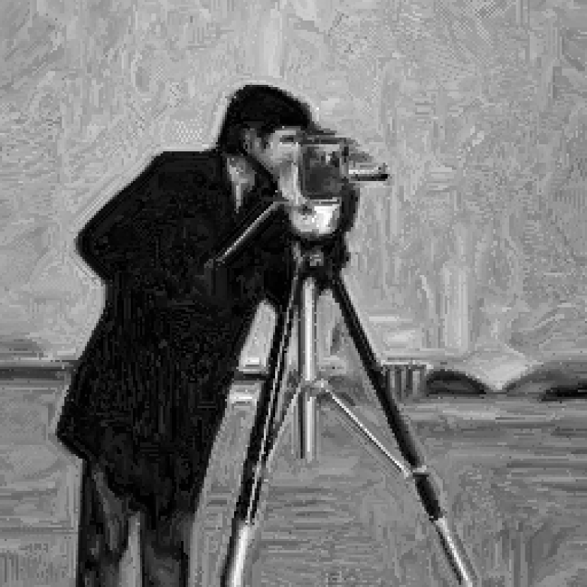
Output without

subimage accumulation

PSNR = 23.37dB

(c)

Output with

subimage accumulation

PSNR = 26.69dB

Fig. 5: The output of our restoration scheme with and without subimage accumulation. The scheme is applied to the Gaussian denoising task with ${\sigma=50}$, and initialized with BM3D.

3.3 Building the Objective Function

In order to build the objective function, we denote by ${\mathbf{y}\in\mathbb{R}^{N}}$ the column stacked version of the corrupted image, by ${\mathbf{x}\in\mathbb{R}^{N}}$ the desired image, and by ${r(\mathbf{x})}$ the regularization term in Equation (8). Then, the inverse problem is formulated as a weighted sum of the negative log-likelihood term ${f_{L}(\mathbf{x,y})}$, and the regularizer ${r(\mathbf{x})}$. In order to keep ${\mathbf{x}}$ values within the pixel boundaries ${[x_{min},x_{max}]}$ we add to the objective function two penalties: ${p(x_{min}\cdot\mathbf{1},\mathbf{x})}$ and ${p(\mathbf{x},x_{max}\cdot\mathbf{1})}$. Therefore, the reconstruction algorithm is generally formulated as the following minimization problem:

$$\min\limits_{\mathbf{x}}\quad f_{L}(\mathbf{x,y})+\mu\cdot r(\mathbf{x})+p(x_{min}\cdot\mathbf{1},\mathbf{x})+p(\mathbf{x},x_{max}\cdot\mathbf{1}),$$ (9)

where ${p(\mathbf{u},\mathbf{w})}$ is defined as:

$$p(\mathbf{u},\mathbf{w})=c\sum_{k=1}^{N}\left(|u_{k}-w_{k}|+u_{k}-w_{k}\right)\;.$$ (10)

Each component of ${p(\mathbf{u},\mathbf{w})}$ is greater than zero when ${u_{k}>w_{k}}$, and grows with the difference ${u_{k}-w_{k}}$. The parameter $c$ controls the strength with which we enforce this penalty.

In order to use a derivative based optimization method for solving the obtained minimization problem, the energy function in Equation (9) is smoothed by replacing the absolute values ${|\cdot|}$ with ${\rho(\cdot,\epsilon)}$, when

$$\rho(w,\epsilon)=\frac{w^{2}}{|w|+\epsilon}\;.$$ (11)

In other words, ${r(\mathbf{x})}$ is replaced with its smooth version ${r_{sm}(\mathbf{x},\epsilon)}$, and ${p(\mathbf{u},\mathbf{w})}$ with ${p_{sm}(\mathbf{u},\mathbf{w},\epsilon)}$, where:

$$r_{sm}(\mathbf{x},\epsilon)=\sum_{i=1}^{\sqrt{n}}\sum_{j=1}^{\sqrt{n}}\sum_{k=1}^{N}\rho\left(\left[MLPS_{i,j}\mathbf{x}\right]_{k},\epsilon\right)\;,$$ (12)

and

$$p_{sm}(\mathbf{u},\mathbf{w},\epsilon)=c\sum_{k=1}^{N}\left[\rho(u_{k}-w_{k},\epsilon)+u_{k}-w_{k}\right]\;.$$ (13)

The function ${\rho(w,\epsilon)}$ is smooth and convex (in ${w}$), since

$$\frac{d\rho(w)}{dw}=\frac{w|w|+2w\epsilon}{(|w|+\epsilon)^{2}}\quad\text{and}\quad\frac{d^{2}\rho(w)}{dw}=\frac{2\epsilon^{2}}{(|w|+\epsilon)^{3}}\;.$$

In all our simulations we solve the unconstrained smoothed optimization problem using L-BFGS method [16] implemented in minFunc [15]. The minimization task runs approximately 200-300 iterations. For $256\times 256$ images it takes around 1-2 minutes, and for $512\times 512$ images 5-10 minutes. Our simulations ran on Intel i7 core with 16GB RAM. The code of Algorithm 1 and parts of the code of the minFunc are implemented in C. The rest of the code is implemented in Matlab.

4 Experimental Results

4.1 Gaussian Denoising

For the Gaussian denoising task, the smooth unconstrained optimization problem is formulated as:

$$\min\limits_{\mathbf{x}}\quad\frac{1}{2}\left\|\mathbf{x}-\mathbf{y}\right\|_{2}^{2}+\mu\cdot r_{sm}(\mathbf{x},\epsilon_{r})+p_{sm}(\mathbf{0},\mathbf{x},\epsilon_{p})+p_{sm}(\mathbf{x},\mathbf{1},\epsilon_{p})\;.$$ (14)

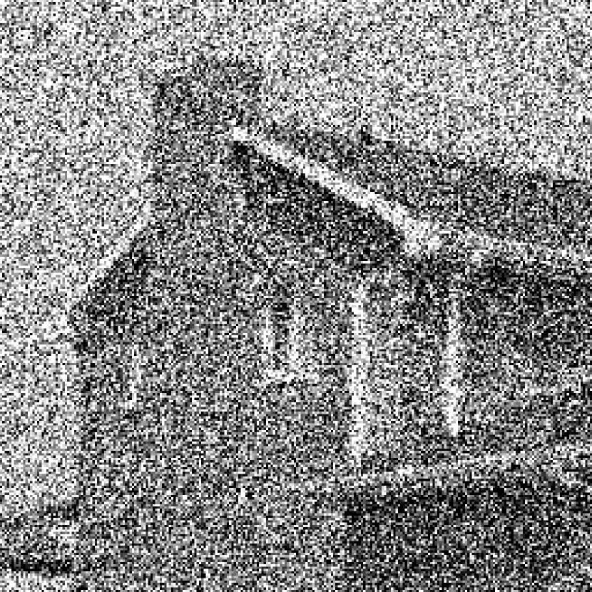
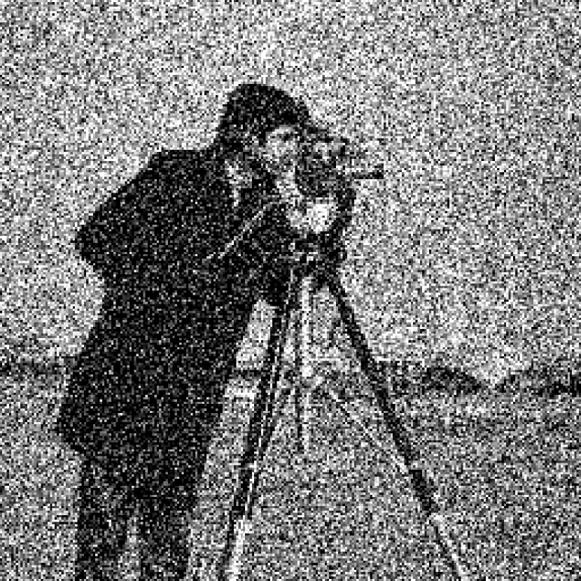
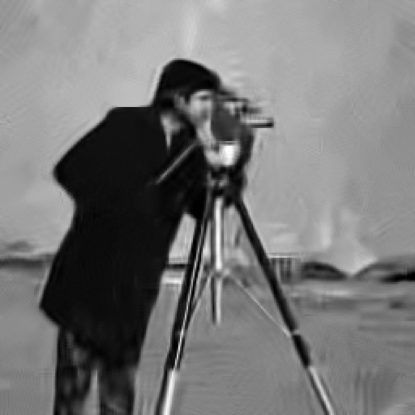
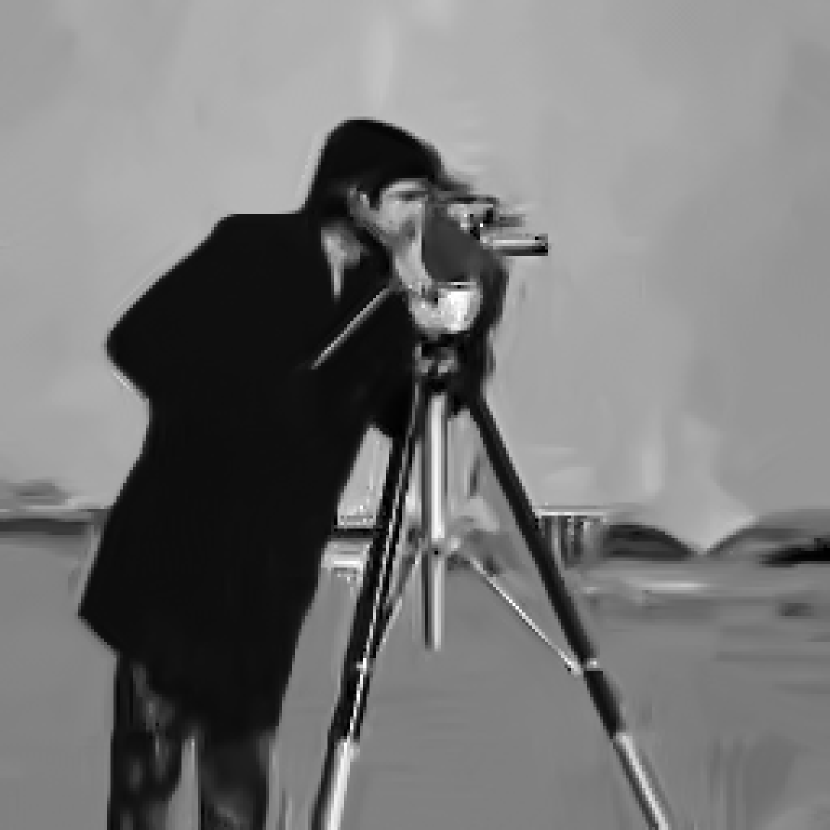
We run denoising experiments for noise levels ${\sigma=25,50,75,\text{ and }100}$. Our scheme is initialized with the output of the BM3D algorithm [4], i.e. the ordering ${\Omega}$ is calculated using the BM3D output. The simulation parameters are summarized in tables 1 and 2. In table 3 we bring quantitative results of these experiments. For each test we compare the PSNR achieved by our scheme with the one referring to the initial images and show the improvement. Note that we do not bring SSIM measure of quality in this table, simply because the conclusions these values lead to are the same as the ones drawn from the PSNR. Examples of qualitative results are shown in Figure 6. For ${\sigma=50}$ and higher, we get an improvement in almost all experiments. For medium noise level, for example ${\sigma=25}$, our scheme does not succeed to improve the PSNR in most of the experiments, because the global patch ordering forces self-similarity on the image patches, and therefore it tends to eliminate distinctive details. In addition, our algorithm does not perform well on image areas that contain sensitive texture or high amount of edges. Examples of such areas are: striped pants in the Barbara image and friction ridges in the fingerprint image.

Along with the experiments described above we also performed the Gaussian denoising experiment (with $\sigma=75$) while replacing the $L_{2}$ distance by the SSIM index. We calculated the SSIM measure of small patches using the algorithm presented in [29] with two differences: (i) we used ${\sqrt{n}\times\sqrt{n}}$ Gaussian weighting function with $\sigma=1.5$ for computing the local statistics (mean, variance and covariance), instead of ${11\times 11}$ Gaussian used in [29]; (ii) the local statistics of any pixel in the patch was calculated using only the pixels that belong to the patch. For example, for computing the local statistics of the top-left pixel of the patch, $x_{1,1}$, we used $1/4$ of the Gaussian, i.e. pixels $x_{i,j}$, where ${1\leq i,j\leq\sqrt{n}/2}$. In fact, full ${\sqrt{n}\times\sqrt{n}}$ Gaussian window was used only for calculating the statistics of the central pixel of the patch. Unfortunately, this scheme led to performance deterioration when compared to the $L_{2}$ option. We believe that the reason for such behavior is this: SSIM ordering minimizes the distance between patches in terms of their mean, variance and covariance, while our regularizer penalizes for distance between pixels. Thus, in this case, the ordering and the regularizer are not consistent with each other. Clearly, this opens up an opportunity to redefine the regularizer to work in terms of the SSIM measure. We leave this as a future extension of our work.

Table 1: Common parameters for Gaussian denoising, debluring, and super-resolution tests.

${\delta}$	${\gamma_{edge}}$	${m_{max}}$	${g_{thr}}$	${\epsilon_{r}}$	${\epsilon_{p}}$	c	${\sqrt{n}}$	B
${10^{6}}$	1.5	20	3.5	${10^{-1}}$	${10^{-3}}$	1	7	121

Table 2: Gaussian denoising parameters per ${\sigma}$.

${\sigma}$	25	50	75	100
${\mu\times 10^{2}}$	${2.5/n}$	${5/n}$	${8/n}$	${12/n}$

(a) Original House

(b) Noisy with ${\sigma=100}$
PSNR = 8.1dB

(c) The initial image (BM3D)
PSNR = 25.87dB

(d) Our output
PSNR = 26.63dB

(e) Original C.man

(f) Noisy with ${\sigma=75}$
PSNR = 10.64dB

(g) The initial image (BM3D)
PSNR = 24.27dB

(h) Our output
PSNR = 24.95dB

Fig. 6: Example of Gaussian denoising results for the images House and Cameraman with ${\sigma=100\text{ and }75}$ respectively.

Table 3: Gaussian denoising results. Results are averaged over five experiments.

$\sigma$ / PSNR	25 / 20.17			50 / 14.15
	BM3D	Our	Improvement	BM3D	Our	Improvement
Cameraman	29.43	29.44	0.01	26.15	26.65	0.50
House	32.88	33.05	0.17	29.64	30.21	0.56
Peppers	30.23	30.38	0.15	26.70	27.09	0.39
Montage	32.32	32.59	0.28	27.79	28.57	0.78
Lena	32.06	31.96	-0.10	29.01	29.13	0.12
Barbara	30.68	30.39	-0.30	27.23	27.15	-0.08
Boats	29.87	29.66	-0.20	26.70	26.81	0.11
Fprint	27.71	27.15	-0.56	24.53	24.22	-0.32
Man	29.59	29.52	-0.07	26.79	26.89	0.11
Couple	29.69	29.68	-0.01	26.45	26.61	0.16
Hill	29.83	29.70	-0.13	27.15	27.22	0.07
Average	30.39	30.32	-0.07	27.10	27.32	0.22
$\sigma$ / PSNR	75 / 10.63			100 / 8.13
	BM3D	Our	Improvement	BM3D	Our	Improvement
Cameraman	24.36	25.01	0.65	23.10	23.73	0.63
House	27.48	28.18	0.69	25.90	26.66	0.77
Peppers	24.71	25.13	0.42	23.27	23.68	0.41
Montage	25.39	26.36	0.97	23.75	24.71	0.97
Lena	27.19	27.41	0.21	25.85	26.14	0.29
Barbara	25.15	25.20	0.05	23.65	23.74	0.09
Boats	25.01	25.17	0.16	23.85	24.03	0.18
Fprint	22.82	22.64	-0.19	21.59	21.50	-0.10
Man	25.29	25.44	0.15	24.21	24.38	0.17
Couple	24.71	24.86	0.14	23.54	23.65	0.11
Hill	25.63	25.76	0.13	24.57	24.71	0.14
Average	25.25	25.56	0.31	23.93	24.27	0.33

4.2 Debluring

For the debluring task the smooth unconstrained optimization problem is the following:

$$\min\limits_{\mathbf{x}}.\quad\frac{1}{2}\left\|H\mathbf{x}-\mathbf{y}\right\|_{2}^{2}+\mu\cdot r_{sm}(\mathbf{x},\epsilon_{r})+p_{sm}(\mathbf{0},\mathbf{x},\epsilon_{p})+p_{sm}(\mathbf{x},\mathbf{1},\epsilon_{p}),$$ (15)

where ${H}$ is a blur matrix.

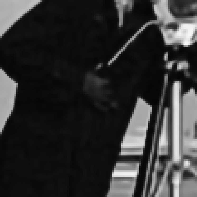
We repeat the experiments reported in [12]. The blur parameters for each experiment, PSF (point spread function) ${h(x_{1},x_{2})}$ and ${\sigma^{2}}$ of the noise, are summarized in table 4. The PSFs are normalized so that ${\sum h(i,j)=1}$. Our scheme is initialized with the output of the IDD-BM3D algorithm [12]. The simulation parameters are summarized in tables 1 and 5. In table 6 we bring quantitative results of the deblurring experiments. For each we compare the PSNR achieved by our scheme with one of the initial images and show the improvement. Examples of qualitative results are shown in Figure 7. Our algorithm improved the image quality in most experiments.

Table 4: Blur and noise variance used in each scenario.

Scenario	PSF	${\sigma^{2}}$
1	${1/(1+x_{1}^{2}+x_{2}^{2}),x_{1},x_{2}=-7,\ldots,7}$	2
2	${1/(1+x_{1}^{2}+x_{2}^{2}),x_{1},x_{2}=-7,\ldots,7}$	8
3	${9\times 9}$ uniform	${\approx 0.3}$
4	${[1\ 4\ 6\ 4\ 1]^{T}[1\ 4\ 6\ 4\ 1]/256}$	49
5	Gaussian with ${std=1.6}$	4
6	Gaussian with ${std=0.4}$	64

Table 5: Debluring parameters per scenario

Scenario	1	2	3	4	5	6
${\mu\times 10^{5}}$	${9/n}$	${24/n}$	${1.6/n}$	${140/n}$	${8/n}$	${500/n}$

(a) Original C.man

(b) Blurred (test 5)
PSNR = 23.36

(c) The initial image
(IDD-BM3D)
PSNR = 27.69dB

(d) Our output
PSNR = 28.50dB

(e) Zoom of the initial image (IDD-BM3D)

(f) Zoom of our output

Fig. 7: Example of debluring results of test 5 for the Cameraman image.

Table 6: Debluring results. Results are averaged over five experiments.

Test	Image	BSNR	Input		IDD-BM3D		Our		Improvement
			PSNR	SSIM	PSNR	SSIM	PSNR	SSIM	PSNR	SSIM
1	C.man	31.87	22.23	0.709	31.11	0.891	31.49	0.904	0.38	0.013
	House	29.16	25.61	0.767	35.54	0.889	36.02	0.896	0.48	0.007
	Lena	29.89	27.25	0.882	35.20	0.972	35.63	0.978	0.43	0.006
	Barbara	30.81	23.34	0.795	30.97	0.970	31.09	0.974	0.12	0.003
	Average	30.44	24.61	0.788	33.20	0.931	33.56	0.938	0.35	0.007
2	C.man	25.85	22.16	0.668	29.31	0.862	29.75	0.873	0.44	0.011
	House	23.14	25.46	0.724	33.99	0.869	34.56	0.879	0.57	0.009
	Lena	23.87	27.04	0.872	33.64	0.957	34.12	0.966	0.49	0.008
	Barbara	24.79	23.25	0.789	27.20	0.926	27.29	0.930	0.08	0.004
	Average	24.43	24.47	0.763	31.04	0.904	31.43	0.912	0.39	0.008
3	C.man	40.00	20.77	0.624	31.24	0.899	31.17	0.910	-0.08	0.011
	House	40.00	24.11	0.697	36.98	0.918	37.57	0.928	0.60	0.009
	Lena	40.00	25.84	0.829	34.74	0.968	35.14	0.973	0.40	0.004
	Barbara	40.00	22.49	0.737	28.53	0.933	28.31	0.930	-0.23	-0.003
	Average	40.00	23.30	0.722	32.87	0.930	33.05	0.935	0.18	0.006
4	C.man	18.53	24.63	0.609	28.63	0.858	29.21	0.873	0.58	0.014
	House	15.99	28.08	0.631	33.85	0.868	34.41	0.879	0.57	0.011
	Lena	16.47	28.81	0.903	33.76	0.957	34.29	0.967	0.52	0.010
	Barbara	17.35	24.22	0.849	26.09	0.908	26.17	0.913	0.07	0.005
	Average	17.17	26.44	0.748	30.58	0.898	31.02	0.908	0.44	0.010
5	C.man	29.19	23.36	0.734	27.69	0.858	28.58	0.873	0.88	0.015
	House	26.61	27.82	0.794	33.55	0.874	34.17	0.883	0.62	0.009
	Lena	27.18	29.16	0.928	34.00	0.968	34.38	0.973	0.38	0.005
	Barbara	28.07	23.77	0.831	24.93	0.883	25.01	0.886	0.07	0.003
	Average	27.77	26.03	0.822	30.04	0.896	30.53	0.904	0.49	0.008
6	C.man	17.76	29.83	0.703	34.69	0.932	34.89	0.939	0.21	0.007
	House	15.15	30.00	0.682	37.08	0.920	36.74	0.911	-0.34	-0.010
	Lena	15.52	30.02	0.911	36.34	0.972	36.32	0.972	-0.02	0.000
	Barbara	16.59	29.78	0.939	35.22	0.979	35.21	0.980	-0.01	0.000
	Average	16.36	29.91	0.809	35.83	0.951	35.79	0.951	-0.04	-0.001

4.3 Super-Resolution

For the single image Super-Resolution (SR) task, our problem is:

$$\min\limits_{\mathbf{x}}\quad\frac{1}{2}\left\|RH\mathbf{x}-\mathbf{y}\right\|_{2}^{2}+\mu\cdot r_{sm}(\mathbf{x},\epsilon_{r})+p_{sm}(\mathbf{0},\mathbf{x},\epsilon_{p})+p_{sm}(\mathbf{x},\mathbf{1},\epsilon_{p}),$$ (16)

where ${H}$ blurs the high resolution image with a ${7\times 7}$ Gaussian kernel with standard deviation 1.6, and ${R}$ downsamples the image by a scaling factor 3 in each pixel. In addition, Gaussian noise with ${\sigma=5}$ is added to the low resolution image.

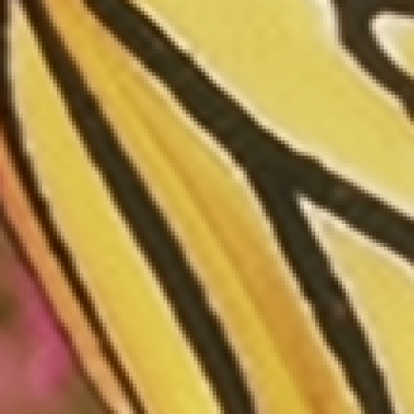
We repeat the experiments reported in  [11], including both noiseless and noisy cases. Our scheme is initialized with output of NCSR algorithm [11]. The simulation parameters are summarized in tables 1 and 7. In table 8 are shown the quantitative results of the SR experiments. Qualitative results are shown in Figure 8. Our algorithm improves the image quality almost in all experiments.

Table 7: Super-resolution parameters per test

Test	Noiseless	Noisy
${\mu\times 10^{5}}$	${1/n}$	${9/n}$

(a) Original Butterfly

(b) Low resolution

(c) The initial image (NSCR)
PSNR = 28.11dB

(d) Our output
PSNR = 29.41dB

(e) Zoom of the initial image (NSCR)

(f) Zoom of our output

Fig. 8: Example of super-resolution (without noise) results for the Butterfly image.

Table 8: Super-Resolution results. Results are averaged over five noise realizations.

Noiseless
Image	NCSR		Our		Improvement
	PSNR	SSIM	PSNR	SSIM	PSNR	SSIM
Butterfly	28.11	0.916	29.43	0.932	1.32	0.017
Flower	29.51	0.856	29.82	0.865	0.31	0.009
Girl	33.36	0.827	33.36	0.824	0.00	-0.003
Parthenon	27.18	0.751	25.39	0.757	0.21	0.006
Parrot	30.52	0.914	31.02	0.921	0.50	0.006
Raccoon	29.28	0.771	29.41	0.766	0.13	-0.004
Bike	24.75	0.803	25.15	0.815	0.40	0.011
Hat	31.25	0.870	31.58	0.877	0.33	0.007
Plants	34.00	0.918	34.60	0.924	0.61	0.006
Average	29.81	0.847	30.23	0.853	0.42	0.006
Noisy
Image	NCSR		Our		Improvement
	PSNR	SSIM	PSNR	SSIM	PSNR	SSIM
Butterfly	26.87	0.888	28.00	0.903	1.13	0.15
Flower	28.08	0.793	28.44	0.807	0.36	0.14
Girl	32.02	0.764	32.10	0.767	0.07	0.004
Parthenon	26.38	0.699	26.63	0.710	0.25	0.010
Parrot	29.51	0.877	29.86	0.879	0.35	0.003
Raccoon	28.02	0.681	28.14	0.689	0.12	0.008
Bike	23.79	0.737	24.28	0.760	0.49	0.023
Hat	29.96	0.824	30.37	0.830	0.41	0.006
Plants	31.74	0.859	32.22	0.866	0.49	0.006
Average	28.49	0.791	28.89	0.801	0.41	0.010

4.4 Poisson denoising

The Poisson negative log-likelihood is given by the following formula:

$$f_{poiss}(\mathbf{x},\mathbf{y})=\sum\limits_{k=1}^{N}f_{k}(x_{k})\;,$$ (17)

where

$$f_{k}(x)=-y_{k}\cdot log(x)+x\;.$$

Since ${f_{k}(x)}$ are not defined for negative ${x}$ values, we extrapolate for ${x<\epsilon}$ using the second order Taylor series:

$$\tilde{f}_{k}(x,\epsilon)=\begin{cases}f_{k}(x)&x\geq\epsilon\;,\\ f_{k}(\epsilon)+f_{k}^{\prime}(\epsilon)(x-\epsilon)+\frac{1}{2}f_{k}^{\prime\prime}(\epsilon)(x-\epsilon)^{2}&x<\epsilon\;.\end{cases}$$

Then we construct the extrapolated likelihood term, ${\tilde{f}_{poiss}(\mathbf{x},\mathbf{y},\epsilon)}$, as a sum of the $\tilde{f}_{k}(x_{k},\epsilon)$ functions:

$$\tilde{f}_{poiss}(\mathbf{x},\mathbf{y},\epsilon)=\sum\limits_{k=1}^{N}\tilde{f}_{k}(x_{k},\epsilon).$$ (18)

Since the ${\tilde{f}_{k}(x,\epsilon)}$ functions penalize the negative $x$ values when ${y_{k}>0}$, the corresponding $k$-th components of the ${p_{sm}(\mathbf{0},\mathbf{x},\epsilon_{p})}$ function can be omitted. Therefore, the ${p_{sm}(\mathbf{0},\mathbf{x},\epsilon_{p})}$ function is reduced to the ${p_{sm}^{y=0}(\mathbf{u},\mathbf{w},\epsilon)}$ function:

$$p_{sm}^{y=0}(\mathbf{u},\mathbf{w},\epsilon)=c\sum_{k:y_{k}=0}\left[\rho(u_{k}-w_{k},\epsilon)+u_{k}-w_{k}\right]\;.$$ (19)

The difference between the ${p_{sm}(\mathbf{0},\mathbf{x},\epsilon_{p})}$ and ${p_{sm}^{y=0}(\mathbf{u},\mathbf{w},\epsilon)}$ is that the ${p_{sm}^{y=0}(\mathbf{u},\mathbf{w},\epsilon)}$ summarizes only over the components for which ${y_{k}=0}$. Thus, the unconstrained optimization problem for the Poisson denoising is formulated by:

$$\min\limits_{\mathbf{x}}\quad\tilde{f}_{poiss}(\mathbf{x},\mathbf{y},\epsilon_{f})+\mu\cdot r_{sm}(\mathbf{x},\epsilon_{r})+p_{sm}^{y=0}(\mathbf{0},\mathbf{x},\epsilon_{p})+p_{sm}(\mathbf{x},x_{max}\cdot\mathbf{1},\epsilon_{p})\;,$$ (20)

where ${x_{max}}$ is calculated using the peak value: ${x_{max}=peak/max\_pix}$, and $max\_pix$ is the maximum pixel value of the clean image.

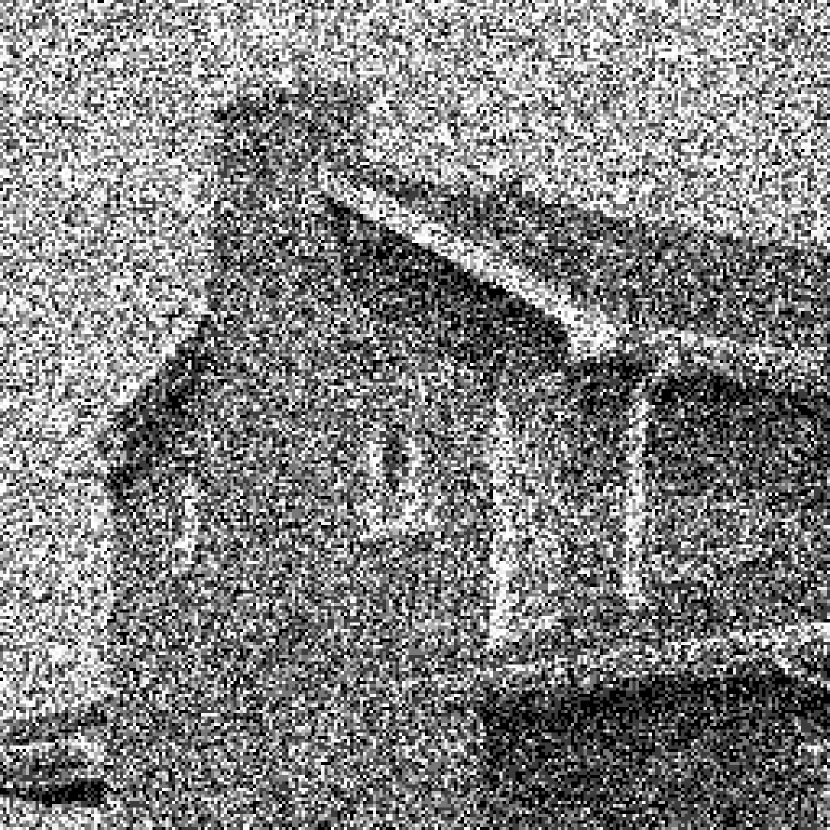
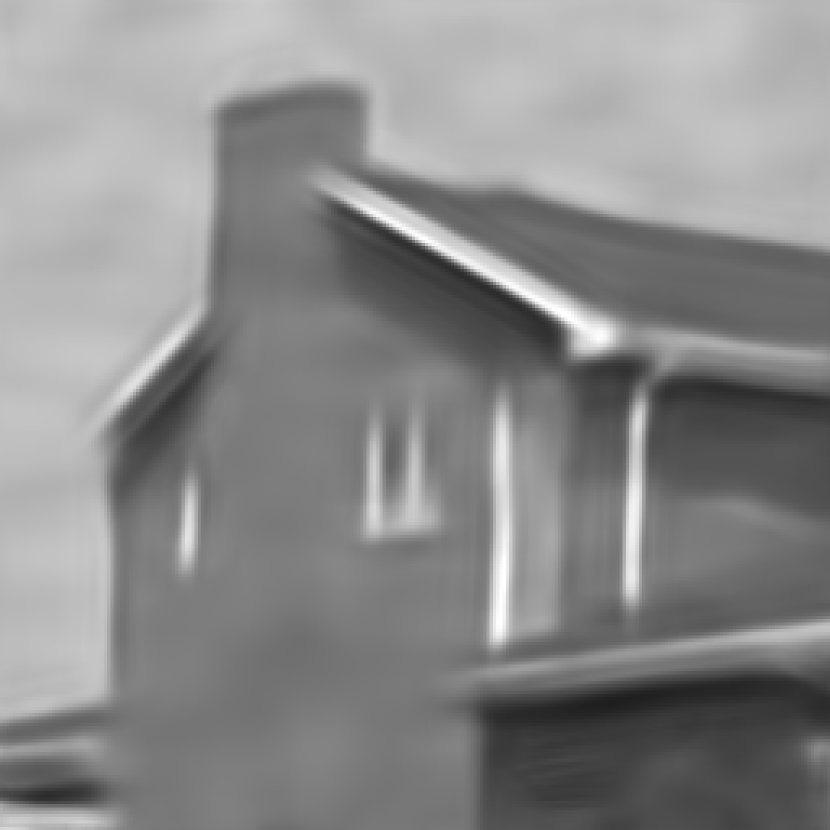
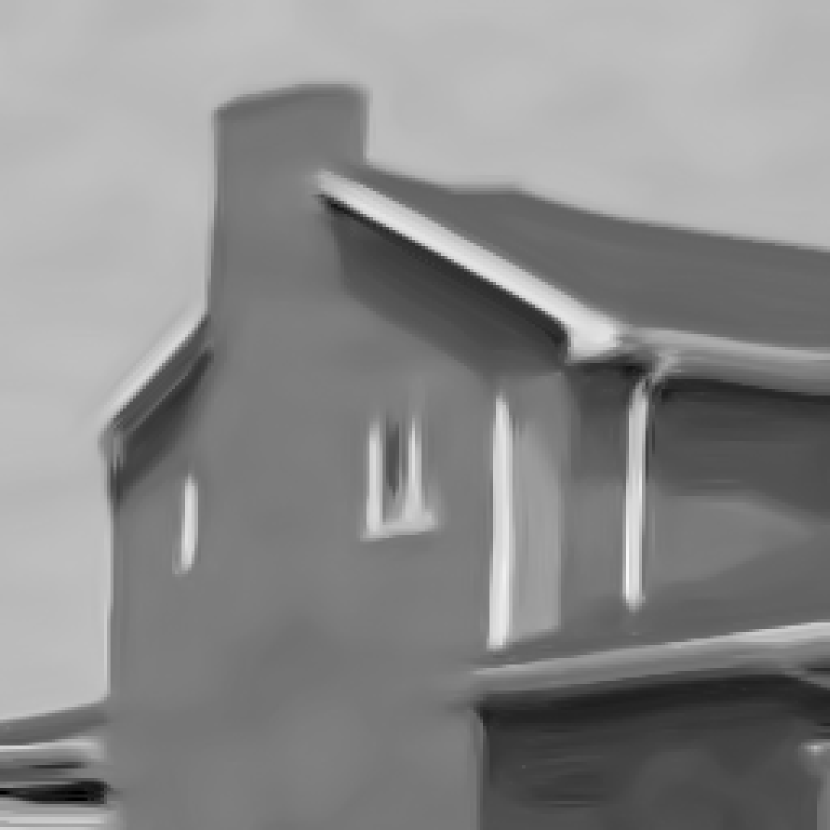
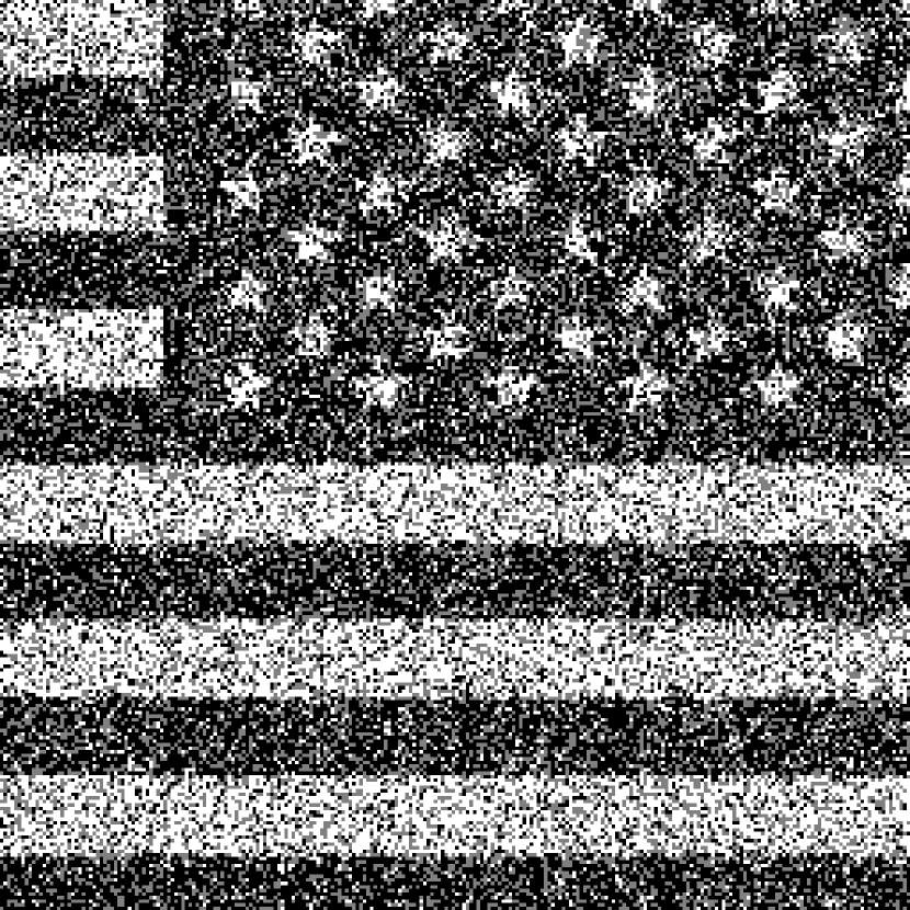
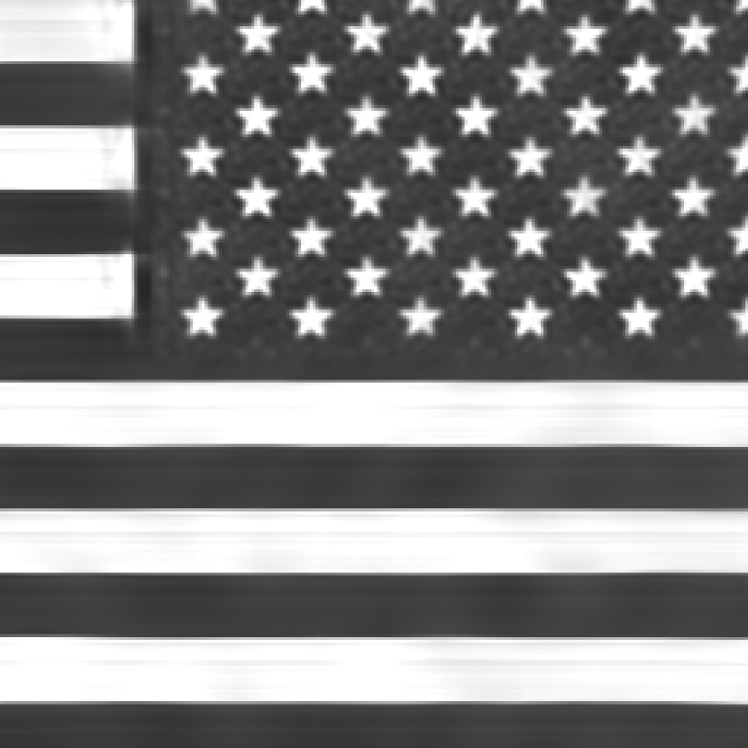
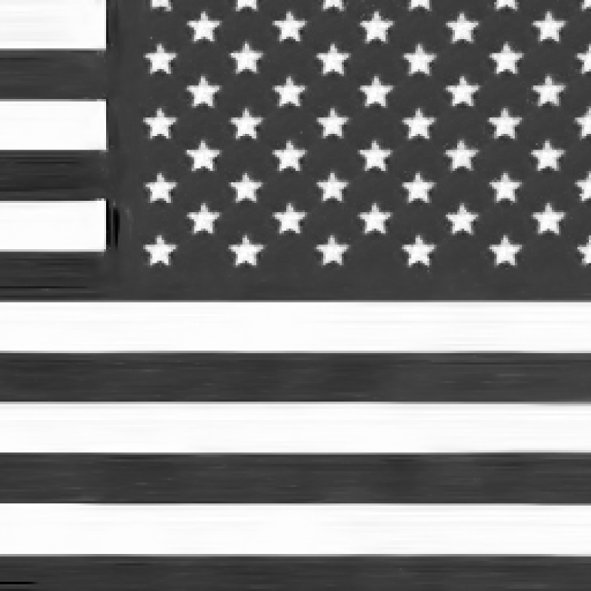
We run experiments for several noise levels – peak = 4, 2, 1, 0.5, 0.2 and 0.1. Our scheme is initialized with the output of the SPDA algorithm [7]. Since SPDA achieves better results for low peaks using binning, we also use binning in the simulations with peaks: 0.5, 0.2 and 0.1. The simulation parameters are summarized in tables 9 and 10. In table 11 we show quantitative results of the experiments. Examples of qualitative results are shown in Figure 9. For the high peak values (peaks 4 and 2 without binning, and peak 0.5 with binning) our algorithm improves the image quality almost in all experiments.

Table 9: Common Poisson denoising parameters.

Bin	${\delta}$	${m_{max}}$	${\epsilon_{r}}$	${\epsilon_{p}}$	${\epsilon_{f}}$	c	${\sqrt{n}}$	B
no	${10^{6}}$	5	${10^{-1}}$	${10^{-3}}$	${10^{-3}}$	1	9	201
${3\times 3}$	${10^{6}}$	5	${10^{-1}}$	${10^{-3}}$	${10^{-3}}$	1	7	101

Table 10: Poisson denoising parameters per peak

Peak	4	2	1	0.5	0.2	0.1
${g_{thr}}$	20	N/A	N/A	10	N/A	N/A
${\gamma_{edge}}$	2.5	1	1	2.5	1	1
${\mu}$	${0.6/n}$	${0.9/n}$	${1.35/n}$	${0.55/n}$	${0.95/n}$	${1.15/n}$

(a) Original House

(b) Noisy with peak = 4
PSNR = 8.40dB

(c) Initialization (SPDA)
PSNR = 25.96dB

(d) Our output
PSNR = 27.00dB

(e) Original Flag

(f) Noisy with peak = 2
PSNR = 5.90dB

(g) Initialization (SPDA)
PSNR = 25.68dB

(h) Our output
PSNR = 26.47dB

Fig. 9: Example of Poisson denoising results for the images House and Flag with peak = 4 and 2 respectively.

Table 11: Poisson denoising results. Results are averaged over five experiments. For each method, the first row presents the reconstruction PSNR, and the second row shows the SSIM measure.

Peak	Method	Bridge	Camera	Flag	House	Peppers	Saturn	Swoosh	Average
4	SPDA	20.55	21.87	26.75	26.02	22.02	31.03	32.67	25.85
		0.367	0.673	0.883	0.753	0.699	0.853	0.960	0.741
	Our	20.92	22.84	28.35	27.15	23.68	31.43	33.71	26.87
		0.398	0.664	0.905	0.783	0.726	0.905	0.969	0.764
	Impr.	0.37	0.97	1.60	1.13	1.66	0.40	1.03	1.02
		0.031	-0.009	0.023	0.031	0.027	0.052	0.009	0.023
2	SPDA	21.14	21.49	25.41	25.07	21.17	29.36	29.24	24.55
		0.352	0.651	0.864	0.716	0.662	0.820	0.893	0.708
	Our	20.22	21.93	26.30	25.63	21.77	29.41	30.15	25.06
		0.362	0.605	0.894	0.749	0.684	0.871	0.930	0.728
	Impr.	0.08	0.43	0.89	0.56	0.60	0.05	0.91	0.50
		0.010	-0.045	0.029	0.033	0.022	0.050	0.038	0.020
1	SPDA	19.21	20.17	22.69	22.62	19.94	27.02	26.41	22.58
		0.304	0.587	0.821	0.632	0.609	0.778	0.823	0.650
	Our	19.24	20.46	22.36	23.20	19.99	26.93	27.37	22.79
		0.315	0.537	0.819	0.677	0.621	0.826	0.880	0.668
	Impr.	0.03	0.28	-0.33	0.57	0.04	-0.09	0.96	0.21
		0.011	-0.049	-0.001	0.045	0.013	0.048	0.056	0.018
0.5	SPDAbin	18.58	18.94	19.39	21.23	18.60	25.89	26.56	21.31
		0.273	0.548	0.691	0.627	0.543	0.756	0.910	0.621
	Our + bin	18.69	19.68	19.63	21.72	18.92	26.37	27.55	21.79
		0.285	0.558	0.703	0.656	0.571	0.835	0.933	0.649
	Impr.	0.10	0.74	0.24	0.49	0.32	0.48	0.98	0.48
		0.012	0.010	0.012	0.030	0.028	0.079	0.023	0.028
0.2	SPDAbin	17.88	17.97	18.60	19.59	17.57	24.03	23.70	19.91
		0.253	0.478	0.670	0.521	0.492	0.691	0.787	0.556
	Our + bin	17.83	18.29	18.58	20.16	17.56	24.09	24.88	20.20
		0.250	0.500	0.673	0.607	0.523	0.813	0.893	0.609
	Impr.	-0.05	0.31	-0.02	0.58	-0.01	0.05	1.17	0.29
		-0.003	0.023	0.003	0.086	0.031	0.122	0.106	0.053
0.1	SPDAbin	17.04	16.80	16.22	18.78	16.29	21.94	21.99	18.44
		0.222	0.493	0.578	0.567	0.477	0.656	0.827	0.546
	Our + bin	17.10	17.16	16.03	18.91	16.28	21.72	22.38	18.51
		0.227	0.462	0.592	0.590	0.491	0.787	0.874	0.575
	Impr.	0.06	0.36	-0.19	0.13	-0.01	-0.11	0.38	0.07
		0.005	-0.030	0.014	0.024	0.014	0.131	0.047	0.029

5 Discussion

5.1 Relation to the work reported in [1, 2]

There is an interesting connection between the approach presented in this paper and the work reported in [1, 2], which introduced the idea of patch-ordering. This connection is easiest to explain in the context of Gaussian denoising. If in our objective function in Equation (9) we replace the robust statistics ($L_{1}$) regularization with a Euclidean norm ($L_{2}$), remove the penalties $p(x_{min}\cdot\mathbf{1},\mathbf{x})$ and $p(\mathbf{x},x_{max}\cdot\mathbf{1})$, remove the weighting matrix, and do not employ subimage accumulation, we get the following minimization problem

$$\min_{\mathbf{x}}\quad\frac{1}{2}\|\mathbf{x}-\mathbf{y}\|_{2}^{2}+\frac{\mu}{2}\|LP\mathbf{x}\|^{2}_{2}\;,$$ (21)

which can be rewritten as

$$\min_{\mathbf{x}}\quad\frac{1}{2}\|P\mathbf{x}-P\mathbf{y}\|_{2}^{2}+\frac{\mu}{2}\|LP\mathbf{x}\|^{2}_{2}\;,$$ (22)

since P is unitary. The solution of this problem is

$$\hat{\mathbf{x}}=P^{-1}\left(I+\mu L^{T}L\right)^{-1}P\mathbf{y}\;.$$ (23)

In other words,

$$\hat{x}=P^{-1}HP\mathbf{y}\;,$$ (24)

where $H=\left(I+\mu L^{T}L\right)^{-1}$ is a circulant matrix that represents a convolution filter. Therefore, the image denoising task obtained by the objective function in (21) reduces to applying permutation $P$ on the noisy image $\mathbf{y}$, smoothing the permuted signal $P\mathbf{y}$ with a convolution filter $H$, and obtaining the result by applying the inverse permutation $P^{-1}$. This solution is similar to the basic idea of the scheme in [1], as formulated in Equation (2) in part ii@.

Now, lets add subimage accumulation in order to get closer to the actual scheme used in both our work and [1]. The minimization problem in (21) transforms into

$$\min_{\mathbf{x}}\quad\frac{1}{2}\|\mathbf{x}-\mathbf{y}\|^{2}_{2}+\frac{\mu}{2n}\sum_{i=1}^{\sqrt{n}}\sum_{j=1}^{\sqrt{n}}\left\|LPS_{i,j}\mathbf{x}\right\|^{2}_{2}\;.$$ (25)

If we pad the image by a circular repetition, the $S_{i,j}$ matrices are unitary and circulant. In this case the objective function in Equation (25) can be rewritten as the sum of contributions of all subimages,

$$\min_{\mathbf{x}}\quad\frac{1}{n}\sum_{i=1}^{\sqrt{n}}\sum_{j=1}^{\sqrt{n}}\left(\frac{1}{2}\left\|PS_{i,j}(\mathbf{x}-\mathbf{y})\right\|^{2}_{2}+\frac{\mu}{2}\left\|LPS_{i,j}\mathbf{x}\right\|^{2}_{2}\right)\;,$$ (26)

where the contribution of the subimage $S_{i,j}$ is

$$\frac{1}{2}\left\|PS_{i,j}(\mathbf{x}-\mathbf{y})\right\|^{2}_{2}+\frac{\mu}{2}\left\|LPS_{i,j}\mathbf{x}\right\|^{2}_{2}\;.$$ (27)

The approach taken in this work is to optimize this penalty directly (if we would have chosen to use the $L_{2}$ as a regularizer). In contrast, one could apply a sub-optimal minimization strategy that minimizes the contribution of each subimage independently and averages the obtained values of $\hat{\mathbf{x}}_{i,j}$. In fact, this is closely related to the approach taken in [1]. The result of this sub-optimal approach will be

$$\hat{\mathbf{x}}_{sub\_optimal}=\frac{1}{n}\sum_{i=1}^{\sqrt{n}}\sum_{j=1}^{\sqrt{n}}\hat{\mathbf{x}}_{i,j}=\frac{1}{n}\sum_{i=1}^{\sqrt{n}}\sum_{j=1}^{\sqrt{n}}S^{-1}_{i,j}P^{-1}\left(I+\mu L^{T}L\right)^{-1}PS_{i,j}\mathbf{y}\;,$$ (28)

where $\hat{\mathbf{x}}_{i,j}$ minimizes contribution of the subimage $S_{i,j}$

$$\hat{\mathbf{x}}_{i,j}=S^{-1}_{i,j}P^{-1}\left(I+\mu L^{T}L\right)^{-1}PS_{i,j}\mathbf{y}\;.$$ (29)

Equation (28) can be rewritten as

$$\hat{\mathbf{x}}_{sub\_optimal}=\frac{1}{n}\sum_{i=1}^{\sqrt{n}}\sum_{j=1}^{\sqrt{n}}S^{-1}_{i,j}P^{-1}HPS_{i,j}\mathbf{y}\;,$$ (30)

where $H=\left(I+\mu L^{T}L\right)^{-1}$ is the convolution filter we have seen before. Therefore, the formula in (30) reduces to the following operations: (i) extract all possible subimages using the $S_{i,j}$ operators and apply permutation $P$ on each subimage, (ii) smooth the permuted signals with convolutional filter $H$, (iii) apply inverse permutation $P^{-1}$ on the results, (iv) plug each subimage into its original place and average the results. To conclude, the formula in Equation (30) is reminiscent of the denoising strategy presented in Equation (7) of part ii@ in [1]. We should stress, however, that the work in [1] is not a special case of the method presented in this paper, due to various additional enhancements used in [1], which are not exploited in this work. These include learning the linear filter, cycle-spinning over the choice of the permutation, and more.

The work reported in [2], as well as the presented work here, constructs an objective function with a permutation-based regularization. However, the scheme in [2] uses multiscale decomposition within the regularization, which makes the algorithm quite involved and computationally expensive. As a consequence, our method is simpler than the one proposed in [2], while remaining very effective. In Table 12 we compare the performance of our scheme with the algorithms presented in [1, 2] for the Gaussian denoising problem. In Table 13 we bring a comparison with [2] for image debluring. Tables 12 and 13 show that our method outperforms the scheme in [1], and achieves results that are comparable to the ones reported in [2].

Table 12: A comparison between the results of the proposed scheme for Gaussian denoising and the ones reported in [1] and [2]. The results of the new method are averaged over five experiments.

$\sigma$ / PSNR	25 / 20.17			50 / 14.15
	[1]	[2]	Ours	[1]	[2]	Ours
Lena	31.80	32.26	31.96	28.96	29.30	29.13
Barbara	30.47	30.90	30.39	27.35	27.78	27.15
Boats	29.70	29.88	29.66	26.69	26.91	26.81
Fprint	27.34	27.32	27.15	24.13	24.06	24.22
House	32.54	32.37	33.05	29.64	29.56	30.21
Peppers	30.01	30.33	30.38	26.75	26.93	27.09
Average	30.31	30.51	30.43	27.25	27.42	27.44
$\sigma$ / PSNR	75 / 10.63			100 / 8.13
	[1]	[2]	Ours	[1]	[2]	Ours
Lena	27.22	27.50	27.41	26.01	26.36	26.14
Barbara	25.42	25.82	25.20	24.07	24.46	23.74
Boats	24.99	25.15	25.17	23.90	24.04	24.03
Fprint	22.47	22.47	22.64	21.44	21.53	21.50
House	27.79	27.37	28.18	26.30	25.98	26.66
Peppers	24.72	24.98	25.13	23.21	23.56	23.68
Average	25.44	25.55	25.62	24.16	24.32	24.29

Table 13: A comparison between the results of the proposed scheme for image debluring and the ones reported in [2]. Results of our scheme are averaged over five experiments.

Image	Method	Test 1	Test 2	Test 3	Test 4	Tests 5	Test 6
Lena	[2]	8.56	6.92	8.86	5.52	4.95	6.91
	ours	8.38	7.08	9.30	5.48	5.22	6.30
Barbara	[2]	8.06	4.57	6.01	2.20	1.41	6.06
	ours	7.75	4.04	5.82	1.95	1.24	5.43
House	[2]	10.44	8.79	13.11	6.38	5.95	7.56
	ours	10.41	9.10	13.46	6.33	6.35	6.74
C.man	[2]	9.24	7.38	10.21	4.34	4.68	5.26
	ours	9.26	7.59	10.40	4.58	5.22	5.06
Average	[2]	9.08	6.92	9.55	4.61	4.25	6.45
	ours	8.95	6.96	9.75	4.58	4.50	5.88

5.2 Choosing the TSP solver

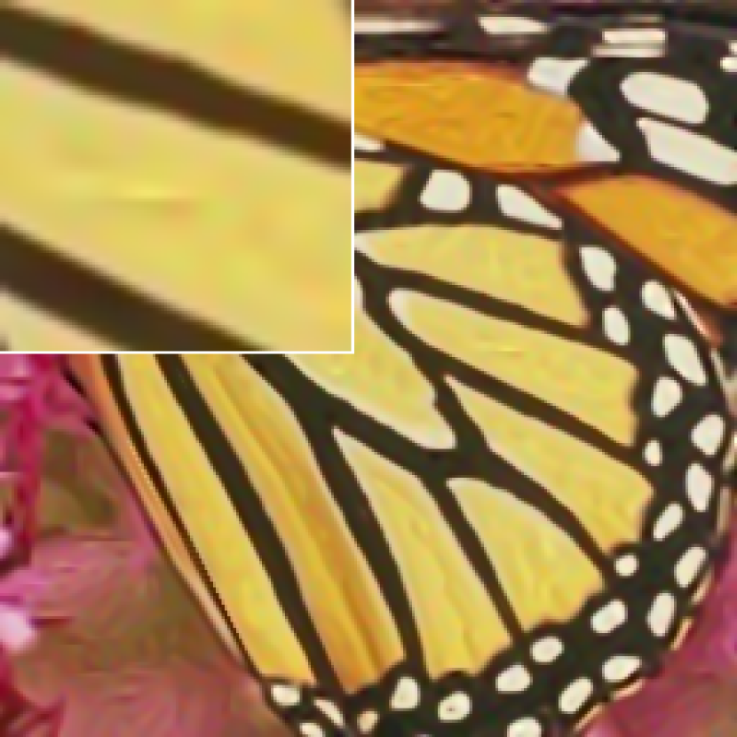
In section 2 we have shown artifact magnification effect when using a deterministic TSP solver. In this section we revisit this phenomena in order to better explain and demonstrate it. Recall that our algorithm starts with some reconstruction result, which is naturally not perfect and thus may contain artifacts. Our regularization relies on a permutation of patches from this image. Thus, a permutation obtained by a more exact TSP solver is in fact creating and magnifying artifacts, since it will assign patches with the same artifacts as neighbors in our ordering. If, on the other hand, one uses the more crude (and somewhat random) ordering that we propose, such similar patches will be separated in the ordering, thus leading to a smoothing out effect of some of these artifacts. In section 2 Figure 1 is showing an example of artifact magnification in the Gaussian denoising test. To complete this presentation, we bring here examples of this effect in other applications. In Figure 10 we compare between the outputs of the proposed method with Lin-Kernighan heuristics and Algorithm LABEL:alg:reordering for the debluring task. In Figures 11 and 12 we do the same comparison for the super-resolution and Poisson denoising tasks respectively. Our conclusion from these experiments is that a more exact TSP solver magnifies artifacts in all applications.

(a) The initial image
(IDD-BM3D)
PSNR = 28.63dB

(b) Output with Lin-Kernighan
PSNR = 28.01dB

(c) Output with Algorithm LABEL:alg:reordering
PSNR = 29.02dB

Fig. 10: The output of our scheme with the Lin-Kernighan heuristics or Algorithm LABEL:alg:reordering for approximating the TSP problem. The reconstruction scheme is applied for test 4 of the image debluring task, and initialized with the IDD-BM3D result.

(a) The initial image (NSCR)
PSNR = 26.87dB

(b) Output with Lin-Kernighan
PSNR = 27.86dB

(c) Output with Algorithm LABEL:alg:reordering
PSNR = 28.00dB

Fig. 11: The output of our scheme with the Lin-Kernighan heuristics or Algorithm LABEL:alg:reordering for approximating the TSP problem. The reconstruction scheme is applied for super-resolution task (with noise $\sigma=5$), and initialized with the NSCR result.

(a) The initial image (SPDA)
PSNR = 25.96dB

(b) Output with Lin-Kernighan
PSNR = 22.76dB

(c) Output with Algorithm LABEL:alg:reordering
PSNR = 27.00dB

Fig. 12: The output of our scheme with the Lin-Kernighan heuristics or Algorithm LABEL:alg:reordering for approximating the TSP problem. The reconstruction scheme is applied for Poisson denoising task with peak = 4, and initialized with the SPDA result.

5.3 Patch Reordering for Better Sparsification

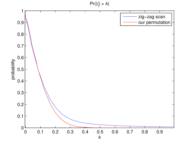
In order to better understand the role of the permutation in the proposed algorithm, we compare the tail distribution functions of the Laplacian result with our ordering versus a zig-zag scan. The Laplacian result are calculated by computing the vector ${\mathbf{l}=MLP\mathbf{x}}$, which is the essence of the regularization term we propose. Using all images listed in Table 3 (referring to the Gaussian denoising test) we compute the cumulative distribution function, ${CDF(k)=Pr(|l_{i}|\leq k)}$ by applying a cumulative sum on the histogram of the components of $|\mathbf{l}|$. For comparison we calculate this $CDF(k)$ while replacing our $P$ with the one obtained by a horizontal zig-zag scan ordering. A comparison of the tail distribution function, ${Pr(|l_{i}|>k)=1-CDF(k)}$ for zig-zag scan and our permutation is shown in Figure 13. As can be seen, our ordering leads to better sparsification of the Laplacian result, when applied to clean images. More specifically, the probability ${Pr(|l_{i}|>k)}$ for the zig-zag scan exhibits a tendency to have more non-zeros, and heavier tail, i.e. bigger values.

Fig. 13: A comparison of the tail distribution functions of the Laplacian result with our ordering versus the zig-zag scan

5.4 Poorly Oredered Pixels

As already mentioned in Section 2, due to greedy nature of the NN heuristics in Algorithm LABEL:alg:reordering, the last part of the reordered image is not as smooth as the rest of the ordering. Nevertheless, the reconstruction results of our algorithm, as shown in the previous section, seem to be of good quality, which may be puzzling. We therefore performed several experiments to better understand this behavior, and here we propose an explanation for this phenomenon.

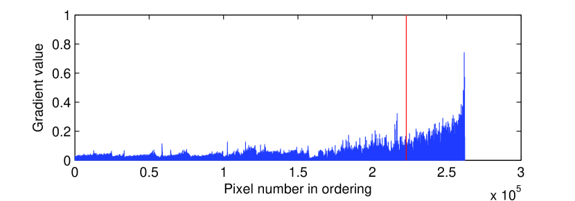
In order to avoid side effects related to the initialization, we start our experiment by computing an oracle-permutation, i.e., applying Algorithm LABEL:alg:reordering on the original clean image (Lena). First we plot a graph of the absolute value of the 1D gradient of the reordered image. As can be seen in Figure 14(a), approximately 15% of the ordering towards the end is not smooth, just as expected. The location of these pixels in the image is shown in Figure 15(b), and as can be seen, these pixels are mostly in edge and texture areas.

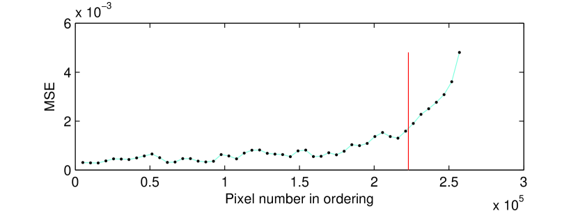
We now perform a Gaussian denoising experiment with $\sigma=75$ ($\mu=0.13$), and our interest is in seeing how the MSE of the output pixels depends on their location in the ordering. We divide the permuted image into 50 groups of pixels with 50% overlap between them, and plot a graph of the average MSE versus location in the ordering, where the x-axis corresponds to the center of each group and the y-axis is the MSE for the groups. This graph is shown in Figure 14(b). Indeed, it is clear that the MSE grows as we tend towards the end of the ordering, implying that the last pixels is ill-treated. However, even for these seemly poorly-served pixels, the obtained MSE is significantly lower than the noise level – in this test, the MSE of the last group is $4.8e{-}3$, where the noise level is $\left(\sigma/255\right)^{2}=86.5e{-}3$. This suggests that even though the last ordered pixels seem to have poor choice of neighbors, their treatment is still rather effective. So, how come this happens?

The answer resides in the sub-image accumulation proposed in our regularization scheme. If a pixel falls in the last part of the ordering, as shown above, it does not imply that this pixel may not be sufficiently close to its neighbors in the patch-ordering, because the poor neighbor assignments are true only in terms of the ordering applied to the central pixels of the patches. The very same poorly-positioned pixels are highly likely to be assigned with effective neighbors in other orderings, as each pixel participates in $n$ such optional permutations. In order to demonstrate this, we check how many pixels fall in the last 15% of all $n$ orderings. For the image Lena this count drops to 3.6% of the pixels, and the location of these pixels is shown in Figure 15(c). These pixels are characterized by the fact that they have no relevant neighbors in the image, regardless of the permutation strategy adopted. As such, they are expected to be ill-treated in the restoration procedure.

(a) Gradient’s absolute value of the reordered pixels.

(b) MSE of the output image.

Fig. 14: (a) The absolute value of the 1D gradient of the reordered Lena image; (b) The MSE of Gaussian denoising of Lena with $\sigma=75$. Last 15% pixels marked with red line.

(a) The original image

(b) Last 15% of the ordering marked Red

(c)

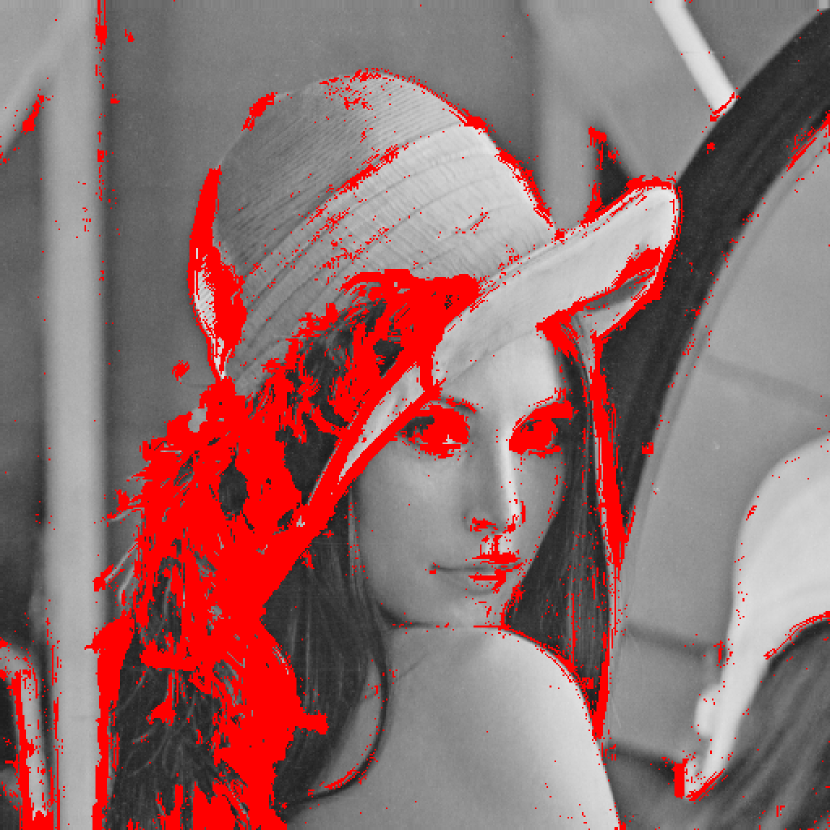
Pixels that fall in last 15%

of all orderings marked Red

Fig. 15: (a) The original image Lena; (b) The last 15% of ordering marked Red; (c) Pixels that fall in the last 15% of all orderings (3.6% in this experiment) marked Red.

5.5 Initialization Strategy

The prime drawback of the proposed method is that it relies on a good initialization. In order to demonstrate this we run a Gaussian denoising experiment on Lena with ${\sigma=50}$ and without BM3D initialization. In this experiment we apply seven rounds of minimization of the penalty function, each followed by a construction of the permutation. The first iteration uses the noisy image itself for building the permutation, while the next iterations rely on the temporary output. We use ${\mu=0.45}$ for the first iteration, ${\mu=0.12}$ for the second, and ${\mu=0.08}$ for the rest. As for the remaining parameters, we used the values listed in table 1. Qualitative and quantitative results of this experiment are shown in Figure 16. Clearly, the result falls short compared to BM3D and other state-of-the-art denoising methods. Thus, our algorithm relies heavily on a good-quality initialization, and further work is required for seeking alternatives to this initialization strategy.

(a) Noisy Lena
PSNR = 14.16dB

(b) Reconstructed: 1’st iteration
PSNR = 24.55dB

(c) Reconstructed: 7’th iteration
PSNR = 27.62dB

(d) BM3D result
PSNR = 29.05dB

Fig. 16: Example of Gaussian denoising results with noisy initialization for the Lena image with ${\sigma=50}$.

6 Conclusion

In this paper we have extended the work in [1], which introduced the concept of patch ordering for handling image denoising and inpainting. Our work exploits the existing interrelation between image patches by building a MAP estimator with permutation-based smoothness-promoting prior on the objective image. The presented scheme is applicable to diverse set of inverse problems in image processing, and in this work we demonstrate its effectiveness for Poisson image denoising, Gaussian image denoising, image deblurring and single image super resolution. In most these tests, our method improved the image quality comparing to the initial image, in some experiments showing an improvement that goes beyong 1dB.

Note that throughout the experiments reported above, we have set the patch ordering only once, based on the initialization image, and then restored a better outcome using our algorithm. In principle, one should iterate this process, by updating the ordering based on the improved image, and then minimizing the MAP functional again. Our initial tests suggest that this is not effective if we are using the same ordering algorithm as described in Section 2. In our future work we plan to investigate alternative ordering that would lead to an overall improvement. In a wider context, we are also seeking ways to depart from the greedy ordering method depicted in Algorithm LABEL:alg:reordering in various ways, such that the final outcome is further improved.

Appendix A L-BFGS

This appendix provides brief description of the L-BFGS algorithm taken from [30]. For this section we denote by ${f(\mathbf{x})}$ a smooth function of ${\mathbf{x}}$, where ${\mathbf{x}\in\mathbb{R}^{n}}$ is a real vector of length ${n}$.

L-BFGS is a limited memory quasi-Newton method, which approximates the inverse of the Hessian matrix instead of calculating the exact one. In additional, it stores only ${m}$ vectors of length ${n}$ (${m\ll n}$) that capture curvature information from recent iterations, instead of saving the full ${n\times n}$ approximation of the Hessian. Each step of L-BFGS is given by

$$\halign to=0.0pt{\relax\global\advance\@IEEEeqncolcnt by 1\relax\begingroup\csname @IEEEeqnarraycolPREl\endcsname#\relax\relax\relax\relax\relax\relax\relax\relax\relax\relax\csname @IEEEeqnarraycolPOSTl\endcsname\relax\relax\relax\relax\relax\relax\relax\relax\relax\relax\endgroup&\relax\global\advance\@IEEEeqncolcnt by 1\relax\begingroup\csname @IEEEeqnarraycolPREl\endcsname#\relax\relax\relax\relax\relax\relax\relax\relax\relax\relax\csname @IEEEeqnarraycolPOSTl\endcsname\relax\relax\relax\relax\relax\relax\relax\relax\relax\relax\endgroup&\relax\global\advance\@IEEEeqncolcnt by 1\relax\begingroup\csname @IEEEeqnarraycolPREl\endcsname#\relax\relax\relax\relax\relax\relax\relax\relax\relax\relax\csname @IEEEeqnarraycolPOSTl\endcsname\relax\relax\relax\relax\relax\relax\relax\relax\relax\relax\endgroup&\global\advance\@IEEEeqncolcnt by 1\relax\bgroup#\egroup&\global\advance\@IEEEeqncolcnt by 1\relax\hbox to\z@\bgroup\hss#\egroup\cr$\displaystyle\mathbf{p}_{k} $\hfil&$\displaystyle\ = \ $\hfil&$\displaystyle-H_{k} \nabla f(\mathbf{x}_{k}) $\hfil&{{}\vrule width=0.0pt,height=0.0pt,depth=0.0pt}&0.0pt{\hss}\cr\penalty 100\vskip 3.0pt\vskip 0.0pt\cr$\displaystyle\mathbf{x}_{k+1} $\hfil&$\displaystyle\ = \ $\hfil&$\displaystyle\mathbf{x}_{k} + \alpha_{k} \mathbf{p}_{k}, \qquad k = 0, 1, 2 \ldots\;, $\hfil&{\vrule width=0.0pt,height=0.0pt,depth=0.0pt}&0.0pt{\hss{\normalcolor(31)}}\cr}$$

where ${\mathbf{x}_{k}}$ is ${\mathbf{x}}$ at iteration ${k}$, ${\alpha_{k}}$ is the step length, and ${H_{k}}$ is the approximation of the inverse of the Hessian of ${f(\mathbf{x})}$ at ${\mathbf{x}_{k}}$ (i.e. ${H^{-1}_{k}}$ is the approximated Hessian). The ${H_{k}}$ matrix is updated at every iteration using the formula

$$H_{k+1}=V^{T}_{k}H_{k}V_{k}+\rho_{k}\mathbf{s}_{k}\mathbf{s}^{T}_{k}\;,$$ (32)

where

$$\rho_{k}=\frac{1}{\mathbf{y}^{T}_{k}\mathbf{s}_{x}},\qquad V_{k}=I-\rho_{k}\mathbf{y}_{k}\mathbf{s}^{T}_{k}\;,$$ (33)

and

$$\mathbf{s}_{x}=\mathbf{x}_{k+1}-\mathbf{x}_{x},\qquad\mathbf{y}_{k}=\nabla f(\mathbf{x}_{k+1})-\nabla f(\mathbf{x}_{k})\;.$$ (34)

Instead of maintaining a full ${H_{k}}$ matrix of size ${n\times n}$, L-BFGS stores it implicitly, by storing ${m}$ vector pairs ${\{\mathbf{s}_{i},\mathbf{y}_{i}\}}$. Given an initial inverse Hessian approximation ${H^{0}_{k}}$, and ${m}$ vector pairs ${\{\mathbf{s}_{i},\mathbf{y}_{i}\},\ i=k-m,...,k-1}$, the ${H_{k}}$ matrix can be found by repeated application of Equation (32)

$$\halign to=0.0pt{\relax\global\advance\@IEEEeqncolcnt by 1\relax\begingroup\csname @IEEEeqnarraycolPREl\endcsname#\relax\relax\relax\relax\relax\relax\relax\relax\relax\relax\csname @IEEEeqnarraycolPOSTl\endcsname\relax\relax\relax\relax\relax\relax\relax\relax\relax\relax\endgroup&\global\advance\@IEEEeqncolcnt by 1\relax\bgroup#\egroup&\global\advance\@IEEEeqncolcnt by 1\relax\hbox to\z@\bgroup\hss#\egroup\cr$\displaystyle H_{k} = \left(V^{T}_{k-1} \ldots V^{T}_{k-m} \right) H^{0}_{k} \left(V_{k-m} \ldots V_{k-1} \right) $\hfil&{{}\vrule width=0.0pt,height=0.0pt,depth=0.0pt}&0.0pt{\hss}\cr\penalty 100\vskip 3.0pt\vskip 4.0pt\cr$\displaystyle+\> \rho_{k-m}\left(V^{T}_{k-1} \ldots V^{T}_{k-m+1} \right) \mathbf{s}_{k-m} \mathbf{s}^{T}_{k-m} \left(V_{k-m+1} \ldots V_{k-1} \right) $\hfil&{{}\vrule width=0.0pt,height=0.0pt,depth=0.0pt}&0.0pt{\hss}\cr\penalty 100\vskip 3.0pt\vskip 4.0pt\cr$\displaystyle+\> \rho_{k-m}\left(V^{T}_{k-1} \ldots V^{T}_{k-m+2} \right) \mathbf{s}_{k-m+1} \mathbf{s}^{T}_{k-m+1} \left(V_{k-m+2} \ldots V_{k-1} \right) $\hfil&{{}\vrule width=0.0pt,height=0.0pt,depth=0.0pt}&0.0pt{\hss}\cr\penalty 100\vskip 3.0pt\vskip 4.0pt\cr$\displaystyle+\> \ldots$\hfil&{{}\vrule width=0.0pt,height=0.0pt,depth=0.0pt}&0.0pt{\hss}\cr\penalty 100\vskip 3.0pt\vskip 4.0pt\cr$\displaystyle+\> \rho_{k-1} \mathbf{s}_{k-1} \mathbf{s}^{T}_{k-1} \;. $\hfil&{\vrule width=0.0pt,height=0.0pt,depth=0.0pt}&0.0pt{\hss{\normalcolor(35)}}\cr}$$

Therefore, the product ${H_{k}\nabla f(\mathbf{x}_{k})}$ can be obtained by a recursive algorithm that involves vector multiplications and summations (Algorithm LABEL:alg:l_bfgs_two_loops).

After each step of L-BFGS, the oldest vector pair ${\{\mathbf{s}_{k-m},\mathbf{y}_{k-m}\}}$ is deleted from memory and replaced by the new pair ${\{\mathbf{s}_{k},\mathbf{y}_{k}\}}$ obtained using Equation (34). At each step of the algorithm, ${\alpha_{k}}$ is chosen to satisfy the Wolfe conditions

$$\halign to=0.0pt{\relax\global\advance\@IEEEeqncolcnt by 1\relax\begingroup\csname @IEEEeqnarraycolPREr\endcsname#\relax\relax\relax\relax\relax\relax\relax\relax\relax\relax\csname @IEEEeqnarraycolPOSTr\endcsname\relax\relax\relax\relax\relax\relax\relax\relax\relax\relax\endgroup&\relax\global\advance\@IEEEeqncolcnt by 1\relax\begingroup\csname @IEEEeqnarraycolPREc\endcsname#\relax\relax\relax\relax\relax\relax\relax\relax\relax\relax\csname @IEEEeqnarraycolPOSTc\endcsname\relax\relax\relax\relax\relax\relax\relax\relax\relax\relax\endgroup&\relax\global\advance\@IEEEeqncolcnt by 1\relax\begingroup\csname @IEEEeqnarraycolPREl\endcsname#\relax\relax\relax\relax\relax\relax\relax\relax\relax\relax\csname @IEEEeqnarraycolPOSTl\endcsname\relax\relax\relax\relax\relax\relax\relax\relax\relax\relax\endgroup&\global\advance\@IEEEeqncolcnt by 1\relax\bgroup#\egroup&\global\advance\@IEEEeqncolcnt by 1\relax\hbox to\z@\bgroup\hss#\egroup\cr\hfil$\displaystyle f(\mathbf{x}_{k} + \alpha_{k} \mathbf{p}_{k})$&\hfil$\displaystyle\ \leq\ $\hfil&$\displaystyle f(\mathbf{x}_{k}) + c_{1} \alpha_{k} \nabla f(\mathbf{x}_{k})^{T} \mathbf{p}_{k} $\hfil&{{}\vrule width=0.0pt,height=0.0pt,depth=0.0pt}&0.0pt{\hss{\normalcolor(36)}}\cr\penalty 100\vskip 3.0pt\vskip 4.0pt\cr\hfil$\displaystyle\nabla f(\mathbf{x}_{k} + \alpha_{k} \mathbf{p}_{k})^{T} \mathbf{p}_{k} $&\hfil$\displaystyle\ \geq\ $\hfil&$\displaystyle c_{2} \nabla f(\mathbf{x}_{k})^{T} \mathbf{p}_{k} \;. $\hfil&{\vrule width=0.0pt,height=0.0pt,depth=0.0pt}&0.0pt{\hss}\cr}$$

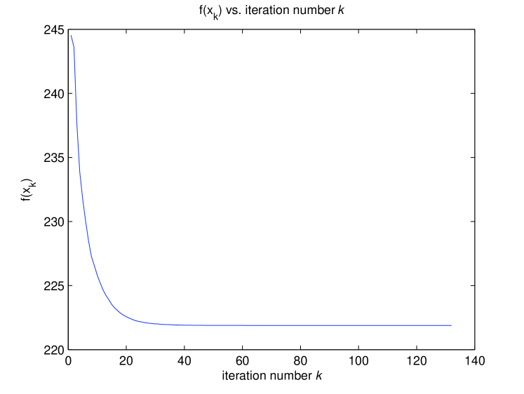
L-BFGS is summarized in Algorithm LABEL:alg:l_bfgs. In our simulations we used minFunc implementation [16] with ${m=8}$. Example of a typical L-BFGS convergence graph is shown in Figure 17.

Fig. 17: Example of L-BFGS convergence: ${f(\mathbf{x}_{k})}$ vs. iteration number during Gaussian denoising of Peppers image with ${\sigma=25}$.

References

- [1] I. Ram, M. Elad, and I. Cohen, “Image processing using smooth ordering of its patches,” Image Processing, IEEE Transactions on, vol. 22, no. 7, pp. 2764–2774, July 2013.
- [2] I. Ram, I. Cohen, and M. Elad, “Patch-ordering-based wavelet frame and its use in inverse problems,” Image Processing, IEEE Transactions on, vol. 23, no. 7, pp. 2779–2792, July 2014.
- [3] M. Elad and M. Aharon, “Image denoising via sparse and redundant representations over learned dictionaries,” Image Processing, IEEE Transactions on, vol. 15, no. 12, pp. 3736–3745, Dec 2006.
- [4] K. Dabov, A. Foi, V. Katkovnik, and K. Egiazarian, “Image denoising by sparse 3-d transform-domain collaborative filtering,” Image Processing, IEEE Transactions on, vol. 16, no. 8, pp. 2080–2095, Aug 2007.
- [5] J. Salmon, C.-A. Deledalle, R. Willett, and Z. Harmany, “Poisson noise reduction with non-local pca,” in Acoustics, Speech and Signal Processing (ICASSP), 2012 IEEE International Conference on, March 2012, pp. 1109–1112.
- [6] J. Salmon, Z. Harmany, C.-A. Deledalle, and R. Willett, “Poisson noise reduction with non-local pca,” Journal of Mathematical Imaging and Vision, vol. 48, no. 2, pp. 279–294, 2014. [Online]. Available: http://dx.doi.org/10.1007/s10851-013-0435-6
- [7] R. Giryes and M. Elad, “Sparsity based poisson denoising with dictionary learning,” CoRR, vol. abs/1309.4306, 2013. [Online]. Available: http://arxiv.org/abs/1309.4306
- [8] J. Yang, J. Wright, T. Huang, and Y. Ma, “Image super-resolution via sparse representation,” Image Processing, IEEE Transactions on, vol. 19, no. 11, pp. 2861–2873, Nov 2010.
- [9] G. Yu, G. Sapiro, and S. Mallat, “Solving inverse problems with piecewise linear estimators: From gaussian mixture models to structured sparsity,” Image Processing, IEEE Transactions on, vol. 21, no. 5, pp. 2481–2499, May 2012.
- [10] D. Zoran and Y. Weiss, “From learning models of natural image patches to whole image restoration,” in Computer Vision (ICCV), 2011 IEEE International Conference on, Nov 2011, pp. 479–486.
- [11] W. Dong, L. Zhang, G. Shi, and X. Li, “Nonlocally centralized sparse representation for image restoration,” Image Processing, IEEE Transactions on, vol. 22, no. 4, pp. 1620–1630, April 2013.
- [12] A. Danielyan, V. Katkovnik, and K. Egiazarian, “Bm3d frames and variational image deblurring,” Image Processing, IEEE Transactions on, vol. 21, no. 4, pp. 1715–1728, April 2012.
- [13] I. Ram, M. Elad, and I. Cohen, “Generalized tree-based wavelet transform,” Signal Processing, IEEE Transactions on, vol. 59, no. 9, pp. 4199–4209, Sept 2011.
- [14] ——, “Redundant wavelets on graphs and high dimensional data clouds,” Signal Processing Letters, IEEE, vol. 19, no. 5, pp. 291–294, May 2012.
- [15] D. C. Liu and J. Nocedal, “On the limited memory bfgs method for large scale optimization,” Math. Program., vol. 45, no. 3, pp. 503–528, Dec. 1989. [Online]. Available: http://dx.doi.org/10.1007/BF01589116
- [16] M.Schmidt, “minfunc: unconstrained differentiable multivariate optimization in matlab,” 2005. [Online]. Available: http://www.cs.ubc.ca/~schmidtm/Software/minFunc.html
- [17] P. Milanfar, “A tour of modern image filtering: New insights and methods, both practical and theoretical,” Signal Processing Magazine, IEEE, vol. 30, no. 1, pp. 106–128, Jan 2013.
- [18] A. Kheradmand and P. Milanfar, “A general framework for regularized, similarity-based image restoration,” Image Processing, IEEE Transactions on, vol. 23, no. 12, pp. 5136–5151, Dec 2014.
- [19] J. Boulanger, C. Kervrann, P. Bouthemy, P. Elbau, J.-B. Sibarita, and J. Salamero, “Patch-based nonlocal functional for denoising fluorescence microscopy image sequences,” Medical Imaging, IEEE Transactions on, vol. 29, no. 2, pp. 442–454, Feb 2010.
- [20] G. Peyré, S. Bougleux, and L. D. Cohen, “Non-local regularization of inverse problems,” Inverse Problems and Imaging, vol. 5, no. 2, pp. 511–530, 2011.
- [21] A. Elmoataz, O. Lezoray, and S. Bougleux, “Nonlocal discrete regularization on weighted graphs: A framework for image and manifold processing,” Image Processing, IEEE Transactions on, vol. 17, no. 7, pp. 1047–1060, July 2008.
- [22] S. Bougleux, A. Elmoataz, and M. Melkemi, “Local and nonlocal discrete regularization on weighted graphs for image and mesh processing,” International Journal of Computer Vision, vol. 84, no. 2, pp. 220–236, 2009.
- [23] X. Liu, D. Zhai, D. Zhao, G. Zhai, and W. Gao, “Progressive image denoising through hybrid graph laplacian regularization: A unified framework,” Image Processing, IEEE Transactions on, vol. 23, no. 4, pp. 1491–1503, April 2014.
- [24] S. Haque, G. Pai, and V. Govindu, “Symmetric smoothing filters from global consistency constraints,” Image Processing, IEEE Transactions on, vol. 24, no. 5, pp. 1536–1548, May 2015.
- [25] Y. Romano and M. Elad, “Boosting of image denoising algorithms,” SIAM Journal on Imaging Sciences, vol. 8, no. 2, pp. 1187–1219, 2015.
- [26] T. H. Cormen, C. E. Leiserson, R. L. Rivest, and C. Stein, “Introduction to algorithms 2nd edition,” 2001.
- [27] S. Lin and B. W. Kernighan, “An effective heuristic algorithm for the traveling-salesman problem,” Operations Research, vol. 21, no. 2, pp. 498–516, 1973. [Online]. Available: http://dx.doi.org/10.1287/opre.21.2.498
- [28] D. Applegate, R. Bixby, V. Chvátal, and W. Cook, “Concorde tsp solver,” 2006. [Online]. Available: http://www.tsp.gatech.edu/concorde
- [29] Z. Wang, A. Bovik, H. Sheikh, and E. Simoncelli, “Image quality assessment: from error visibility to structural similarity,” Image Processing, IEEE Transactions on, vol. 13, no. 4, pp. 600–612, April 2004.
- [30] J. Nocedal and S. Wright, Numerical Optimization, ser. Springer Series in Operations Research. Springer, 1999. [Online]. Available: http://books.google.de/books?id=epc5fX0lqRIC