Snowflake geometry in CAT(0) groups

Abstract.

We construct CAT(0) groups containing subgroups whose Dehn functions are given by $x^{s}$, for a dense set of numbers $s\in[2,\infty)$. This significantly expands the known geometric behavior of subgroups of CAT(0) groups.

1. Introduction

In this paper we are concerned with the geometry of subgroups of CAT(0) groups. Such subgroups need not be CAT(0) themselves, and in fact this realm includes many instances of exotic or unusual group-theoretic behavior. For example, there exist finitely presented subgroups of CAT(0) groups having unsolvable membership and conjugacy problems [BBMS00, Bri13], or possessing infinitely many conjugacy classes of finite subgroups (implicitly in [FM91], explicitly in [LN03, BCD08]). Many well known examples of groups having interesting homological properties, such as the Stallings–Bieri groups or other Bestvina–Brady kernels, arise naturally as subgroups of CAT(0) groups.

Regarding the geometry, specifically, of subgroups of CAT(0) groups, only a few types of unusual behavior have been observed to date. One common feature to all subgroups of CAT(0) groups is that cyclic subgroups are always undistorted. This constraint immediately rules out a great many examples from being embeddable into CAT(0) groups. The examples found so far with interesting geometric properties have been constructed using fairly sophisticated techniques. Such examples include the hydra groups of [DR13], which are CAT(0) groups possessing free subgroups with extreme distortion; subgroups of CAT(0) groups having exponentional or polynomial Dehn functions [BBMS97, Bri13], [BRS07, ABD⁺13, BGL11]; and subgroups of CAT(0) groups having different homological and ordinary Dehn functions [ABDY13].

Our goal in the present paper is to construct CAT(0) groups containing subgroups that exhibit a wide range of isoperimetric behavior. Our main theorem is the following.

Theorem A.

Let $m,n$ be positive integers such that $\alpha=n\log_{m}(1+\sqrt{2})\geqslant 1$. Then there exists a $6$–dimensional CAT(0) group $G$ which contains a finitely presented subgroup $S$ whose Dehn function is given by $\delta_{S}(x)=x^{2\alpha}$.

Varying $m$ and $n$, the resulting isoperimetric exponents $2\alpha$ form a dense set in the interval $[2,\infty)$. Thus, the isoperimetric spectrum of exponents arising from subgroups of CAT(0) groups resembles, in its coarse structure, that of finitely presented groups generally [BB00].

Contents

1. 1 Introduction
2. 2 Preliminaries
3. 3 Group-theoretic constructions
4. 4 The CAT(0) structure
5. 5 Embedding results
6. 6 Corridor schemes and the balancing property of $V_{T}$
7. 7 Canonical diagrams
8. 8 Snowflake diagrams
9. 9 Folded corridors and subgroup distortion
10. 10 The Dehn function of $S_{T,n}$

The group $S$ in the main theorem is constructed with reference to certain parameters; it is denoted $S_{T,n}$ where $T$ is a finite tree and $n$ is an integer. It will embed into a CAT(0) group denoted $G_{T,n}$.

Comparison with prior constructions of snowflake groups

The construction of the snowflake groups $S_{T,n}$ builds on the methods used in [BBFS09] to construct groups with specified power functions as Dehn functions. The latter groups do not embed into any CAT(0) group, for the simple reason that they contain distorted cyclic subgroups. The same is true for the groups constructed in [SBR02], and many other groups having interesting Dehn functions. Indeed, it is the presence of precisely distorted cyclic subgroups that enables the computation of the Dehn functions in [BBFS09] in the first place.

The basic structure of the groups in [BBFS09] is that of a graph of groups, with vertex groups of cohomological dimension $2$, and infinite cyclic edge groups. The lower bound for the Dehn function was easy to establish, using asphericity of the presentation $2$–complex. The distortion of the cyclic edge groups was then precisely determined, and this distortion estimate led to a matching upper bound for the Dehn function of the ambient group.

If one hopes to embed examples into CAT(0) groups, one cannot have distorted cyclic subgroups. The groups $S_{T,n}$ we construct here are fundamental groups of graphs of groups in which the edge groups are free groups of rank $2$. Moreover, the vertex groups are groups of cohomological dimension $3$, and therefore $S_{T,n}$ does not admit an aspherical presentation. For this reason, establishing the lower bound for the Dehn function of $S_{T,n}$ requires some effort.

The change to free edge groups introduces some major challenges. In [BBFS09], given any element of an edge group, conjugation by the appropriate stable letter resulted in a word $r$ times longer, for a uniform factor $r$. In the Cayley $2$–complex, each edge space had a well defined long side and short side. A key geometric property was that no geodesic could pass from the short side to the long side of any edge space, and back again. It thus became possible to determine the large scale behavior of geodesics, which in turn led to very explicit distance estimates in the group.

In the groups $S_{T,n}$ defined here, the edge groups have monodromy modeled on a hyperbolic free group automorphism. Under this automorphism, some words get longer and some get shorter. It is no longer possible to constrain the behavior of geodesics relative to the Bass-Serre tree for the graph of groups structure as in [BBFS09]. This local stretching and compressing behavior of the automorphism is a phenomenon that was similarly faced in the work of Bridson and Groves in [BG10]. To accommodate this behavior, we rely on a coarser and more robust approach. We begin with the framework used in [BB00], and develop additional techniques for handling the lack of local control over geodesics. These ideas are described in more detail in the subsection “Edge group distortion” near the end of this Introduction.

The embedding trick

The method we use for embedding $S_{T,n}$ into a CAT(0) group is based on a twisting phenomenon for graphs of groups. Suppose $\alpha\colon\thinspace G_{e}\to G_{v}$ is the inclusion map from an edge group to a vertex group, where $e$ is incident to $v$. If one replaces $\alpha$ by $\varphi\circ\alpha$, where $\varphi$ is an automorphism of $\alpha(G_{e})$, then typically one obtains a very different fundamental group. However, if $\varphi$ is the restriction of an inner automorphism of $G_{v}$, then the fundamental group remains unchanged.

The graph of groups structure of the group $S_{T,n}$ incorporates in an essential way the “twisting automorphisms” $\varphi$ just described; properties of these automorphisms influence strongly the geometry of $S_{T,n}$. The presence of twisting accounts for the lack of non-positive curvature and the possibility of larger-than-quadratic isoperimetric behavior.

In order to embed $S_{T,n}$ into a larger group $G_{T,n}$, we give the latter the structure of a graph of groups that is very similar to that of $S_{T,n}$. It has the same underlying graph, somewhat larger edge and vertex groups, and inclusion maps which make use of twisting automorphisms closely related to those in $S_{T,n}$. This is to ensure the existence of a morphism of graphs of groups which induces a homomorphism $S_{T,n}\to G_{T,n}$. Injectivity of this homomorphism is established using a criterion due to Bass [Bas93]; see Lemma 5.1.

The basic trick now is that the vertex group in $G_{T,n}$ has been enlarged specifically to arrange that the twisting automorphisms become inner. Thus the twisting can be undone, without changing the fundamental group. With no twisting, it becomes a simple matter to put a CAT(0) structure on $G_{T,n}$, provided the enlarged vertex group is already CAT(0).

Bieri doubles and the embedding trick

Earlier we referred to examples of subgroups of CAT(0) groups having exponentional or polynomial Dehn functions. The examples from [BBMS97, BRS07] made use of an embedding theorem from [BBMS97]. The authors embed certain doubles of groups into the direct product of a related group and a free group; the latter product may then have a CAT(0) structure, while the embedded subgroup has interesting geometric behavior. The embedded subgroup is called a Bieri double.

It turns out that some instances of this method can be viewed as instances of the embedding trick discussed above, resulting in an alternative way of looking at certain Bieri doubles.

Here is an example, which includes the [BRS07] examples of subgroups of CAT(0) groups having polynomial Dehn functions. Let $N$ be any group with an automorphism $\varphi$, and consider the double of $N\rtimes_{\varphi}{\mathbb{Z}}$ along $N$: $(N\rtimes\langle t_{1}\rangle)\ast_{N}(N\rtimes\langle t_{2}\rangle)$. There is a homomorphism

$$(N\rtimes\langle t_{1}\rangle)\ast_{N}(N\rtimes\langle t_{2}\rangle)\ \to\ (N\rtimes\langle t\rangle)\times\langle u,v\rangle$$

which sends $N$ to $N$, $t_{1}$ to $tu$, and $t_{2}$ to $tv$. The arguments of [BBMS97] show that this map is an embedding.

An alternative viewpoint is to note that the double $(N\rtimes\langle t_{1}\rangle)\ast_{N}(N\rtimes\langle t_{2}\rangle)$ has a graph of groups decomposition ${\mathscr{A}}$ with underlying graph a figure-eight, with all edge and vertex groups $N$, and with monodromy along each loop given by $\varphi$. The elements $t_{1}$ and $t_{2}$ are the two stable letters. The larger group $(N\rtimes\langle t\rangle)\times\langle u,v\rangle$ has a similar decomposition with the same underlying graph, with vertex and edge groups $N\rtimes\langle t\rangle$, with monodromy the identity. In this case $u$ and $v$ are the two stable letters.

This description of the larger group is the “untwisted” presentation for it. If we change the monodromy to be by the automorphism $\varphi\times\operatorname{id}$ of $N\rtimes\langle t\rangle$, then the new graph of groups ${\mathscr{B}}$ still has fundamental group $(N\rtimes\langle t\rangle)\times\langle u,v\rangle$, since $\varphi\times\operatorname{id}$ is conjugation by $t$ in the vertex group $N\rtimes\langle t\rangle$. The two stable letters for this new decomposition are $tu$ and $tv$. There is an obvious morphism of graphs of groups ${\mathscr{A}}\to{\mathscr{B}}$ since $\varphi\times\operatorname{id}$ restricts to $\varphi$ on $N$. The induced map on fundamental groups is exactly the embedding displayed above.

An overview of the construction

Recall that our basic aim is to construct a pair of finitely presented groups $S$ and $G$ such that $G$ is CAT(0), $S$ embeds into $G$, and $S$ has a specified Dehn function. The starting data needed for our constructions is as follows.

First choose a palindromic monotone automorphism $\varphi\colon\thinspace\langle x,y\rangle\to\langle x,y\rangle$ (see Section 2 for these notions). Let $\lambda$ be the Perron-Frobenius eigenvalue of the transition matrix of $\varphi$. Also let $T$ be a finite tree with valence at most $3$, and let $m=\lvert{T}\rvert+1$ (here, $\lvert{T}\rvert$ denotes the number of vertices of $T$). Choose a positive integer $n$ such that $\alpha=n\log_{m}(\lambda)\geqslant 1$. Based on these choices, we define finitely presented groups $S_{T,n}$ and $G_{T,n}$.

These groups are multiple HNN extensions of groups $V_{T}$ and $W_{T}$ respectively, with $m$ stable letters. In Section 3 we define these vertex groups; they are, themselves, fundamental groups of graphs of groups with underlying graph $T$. The group $V_{T}$, in particular, is required to have some very special properties, notably the balancing property. The structure needed to achieve this property also dictates how $W_{T}$ should be constructed.

Briefly, $V_{T}$ has vertex groups isomorphic to $F_{2}\times F_{2}\times F_{2}$, and each such group has three designated peripheral subgroups which are used as edge groups; these edge groups are isomorphic to $F_{2}$. They are the “antidiagonal” copies of $F_{2}$ in each factor $F_{2}\times F_{2}$ in each vertex group.

The group $W_{T}$ is built in a similar way, with the free-by-cyclic group $G=F_{2}\rtimes_{\varphi}{\mathbb{Z}}$ used in place of $F_{2}$; thus the vertex groups are $G\times G\times G$, and the edge groups are isomorphic to $G$. The groups $G$ possess $2$–dimensional CAT(0) structures, by work of Tom Brady [Bra95].

Given the CAT(0) structure on $W_{T}$, the ambient group $G_{T,n}$ can also be made CAT(0), as in the discussion of the Embedding Trick above; see Section 4. When building this CAT(0) structure, we fix the free group automorphism $\varphi$ to be a particular one which is palindromic. Tom Brady’s CAT(0) structure has a symmetry that respects the palindromic nature of $\varphi$. In the case of the other free-by-cyclic groups arising in [Bra95], we believe that analogous symmetries exist (in the palindromic case), but establishing this would take us too far afield. It is for this reason that the exponents in the main theorem involve $1+\sqrt{2}$ (which is $\lambda$ for this choice of $\varphi$). Apart from the CAT(0) statement for $G_{T,n}$, the rest of the paper does not require any particular choice of $\varphi$, and we compute the Dehn functions of $S_{T,n}$ in terms of a general (monotone, palindromic) $\varphi$.

Corridor schemes and $\sigma$–corridors

There are several places where we make use of corridor arguments in van Kampen diagrams. There are many different types of corridors under consideration simultaneously, and these different types are codified as corridor schemes. In particular, the group $V_{T}$ possesses a large number of distinct corridor schemes, which are parametrized by maximal segments $\sigma$ in a tree $\widehat{T}$. Each such segment determines a corridor scheme, whose corridors are called $\sigma$–corridors.

These corridors provide the primary means by which we establish the properties of $V_{T}$ that are needed, such as the balancing property (Proposition 6.7). This latter property is somewhat awkward to explain, but it concerns the distribution of generators in words representing the trivial element. The property has the most force when the generators all lie in peripheral subgroups of $V_{T}$. It implies, for instance, that an element of a peripheral subgroup cannot be expressed efficiently using only generators from other peripheral subgroups; see Remarks 6.8. The balancing property plays a key role in several parts of the paper, most notably in the distortion bound of Proposition 9.7, and also in the area bound for $V_{T}$ given in Proposition 10.3.

Least-area diagrams

In sections 7 and 8 we define families of van Kampen diagrams in order to establish the lower bound for the Dehn function of $S_{T,n}$. We use basic building blocks called canonical diagrams, which are defined for every palindromic word in $\langle x,y\rangle$. These are diagrams over the vertex group $V_{T}$. We then build snowflake diagrams over $S_{T,n}$, using canonical diagrams joined along strips dual to the stable letters of $S_{T,n}$.

To establish the lower bound, we show that all of these diagrams minimize area relative to their boundary words. Proving this requires a detailed study of $\sigma$–corridors and their intersection properties for various $\sigma$.

Edge group distortion

The heart of the computation of the Dehn function of $S_{T,n}$ lies in Proposition 9.7, in which we establish the distortion of the edge groups inside $S_{T,n}$. This argument requires first some properties of folded corridors, analogous to those studied in [BG10] in the context of free-by-cyclic groups. These properties are established in the first half of Section 9, culminating in Lemma 9.5.

Next we establish the bound on edge group distortion. The proof is an inductive proof based on Britton’s Lemma. It falls into two cases, which require very different treatments. In the first case, the proof is based on a method from [BB00]. It is only thanks to the balancing property of $V_{T}$ that this argument can be carried out.

The second case is where the folded corridors and Lemma 9.5 come in. The inductive framework is based on the nested structure of $r_{j}$–corridors in a putative van Kampen diagram. These corridors may appear in two possible orientations, forwards and backwards. Forward-facing corridors present few difficulties and can be handled using the method above based on the balancing property. If there is a backwards-facing $r_{j}$–corridor, then it may introduce undesirable geometric effects that threaten to spoil the inductive calculation. The argument in this case is to show that when this occurs, there will be forward facing corridors just behind the first one, and perfectly matching segments along these corridors, along which any metric distortion introduced by the first corridor is exactly undone.

Computing the Dehn function

Establishing the upper bound for the Dehn function of $S_{T,n}$ proceeds along similar lines as in [BBFS09]. One important step in this argument is a statement about area in the vertex group. This occurs in Proposition 10.3 in the present paper. Due to the more complicated structure of $V_{T}$ (being constructed from free groups), the argument is considerably more involved than the corresponding result in [BBFS09]. It requires many of the tools developed here, such as the balancing property and corridor schemes.

Acknowledgments

Noel Brady acknowledges support from the NSF and from NSF award DMS-0906962. Max Forester acknowledges support from NSF award DMS-1105765.

2. Preliminaries

In this section we review some basic definitions and properties concerning Dehn functions, van Kampen diagrams, and words in the free group.

Dehn functions

Let $G=\langle\,A\mid R\,\rangle$ be a finitely presented group and $w$ a word in the generators $A^{\pm 1}$ representing the trivial element of $G$. We define the area of $w$ to be

$$\operatorname{Area}(w)\ =\ \min\Big{\{}N\in{\mathbb{N}}\ \big{|}\ \exists\text{ equality }w=\prod_{i=1}^{N}u_{j}r_{j}u_{j}^{-1}\text{ freely, where }r_{j}\in R^{\pm 1}\Big{\}}.$$

The Dehn function $\delta(x)$ of the finite presentation $\langle\,A\mid R\,\rangle$ is given by

$$\delta(x)\ =\ \max\Big{\{}\operatorname{Area}(w)\ \big{|}\ w\in\ker(F(A)\to G),\lvert{w}\rvert\leqslant x\Big{\}}$$

where $\lvert{w}\rvert$ denotes the length of the word $w$.

There is an equivalence relation on functions $f\colon\thinspace{\mathbb{N}}\to{\mathbb{N}}$ defined as follows. First, we say that $f\preccurlyeq g$ is there is a constant $C>0$ such that

$$f(x)\ \leqslant\ Cg(Cx)+Cx$$

for all $x\in{\mathbb{N}}$. If $f\preccurlyeq g$ and $g\preccurlyeq f$ then we say that $f$ and $g$ are equivalent, denoted $f\simeq g$. It is not difficult to show that two finite presentations of the same group define equivalent Dehn functions; we therefore speak of “the” Dehn function of $G$, which is well defined up to equivalence.

Remark 2.1.

In order to show that $f\preccurlyeq g$ for non-decreasing functions $f$ and $g$, it is sufficient to prove that $f(n_{i})\leqslant g(n_{i})$ for an unbounded sequence of positive integers $\{n_{i}\}$ such that the ratios $n_{i+1}/n_{i}$ are bounded. For, if $n_{i+1}\leqslant Cn_{i}$ for all $i$ and $x$ is any integer between $n_{i}$ and $n_{i+1}$, say, we have $f(x)\leqslant f(n_{i+1})\leqslant g(n_{i+1})\leqslant g(Cn_{i})\leqslant g(Cx)$. Therefore $f(x)\leqslant Cg(x)$ for all $x$.

Let $X$ be a $2$–dimensional cell complex. We call $X$ a presentation $2$–complex if it has one $0$–cell, and every $2$–cell is attached by a map $f\colon\thinspace S^{1}\to X^{(1)}$ which is regular in the following sense: there is a cell structure for $S^{1}$ such that the restriction of $f$ to each edge maps monotonically over a $1$–cell of $X$.

The presentation $2$–complex of the presentation $\langle\,A\mid R\,\rangle$ has oriented $1$–cells labeled by the generators in $A$, and a $2$–cell for each relator $r$ in $R$, attached via a map $S^{1}\to X^{(1)}$ which traverses edges sequentially, following the word $r$.

Given a presentation $2$–complex $X$, one then has the notion of a van Kampen diagram over $X$. Briefly, a van Kampen diagram for the word $w$ is a contractible, planar $2$–complex with edges labeled by generators, with each $2$–cell boundary word equal to a relator, with outer boundary word $w$. The area of the diagram is the number of its $2$–cells. It is a standard fact that $\operatorname{Area}(w)$ as defined above can be interpreted as the minimal area of a van Kampen diagram over $X$ for $w$. See [Bri02] for details on this interpretation of $\operatorname{Area}(w)$. We refer to [Bri02] for background on Dehn functions generally, and also to [BH99] for background on CAT(0) spaces.

Words and automorphisms

A word $w(x,y)$ is palindromic if $w(x^{-1},y^{-1})=w(x,y)^{-1}$ as words in the free group. An automorphism $\varphi\colon\thinspace\langle x,y\rangle\to\langle x,y\rangle$ is called palindromic if it takes palindromic words to palindromic words. Note that $\varphi$ will be palindromic if the two words $\varphi(x)$, $\varphi(y)$ are palindromic. If $\varphi$ is palindromic, so is $\varphi^{n}$ for any $n\geqslant 1$.

A word $w(x,y)$ is positive if it does not contain occurrences of $x^{-1}$ or $y^{-1}$. It is negative if it does not contain $x$ or $y$. It is monotone if it is positive or negative. Note that monotone words are reduced, and if $w$ is monotone then so is $w^{-1}$. If an automorphism $\varphi$ takes $x$ and $y$ to monotone words of the same kind, then it takes all monotone words to monotone words. We call $\varphi$ monotone if it has this property. The same will then be true of $\varphi^{n}$ for any $n\geqslant 1$. (The inverse $\varphi^{-1}$ will typically not be monotone.)

3. Group-theoretic constructions

In this section we begin by constructing groups $V_{T}$ and $W_{T}$, which will then serve as vertex groups in graph of groups decompositions defining the snowflake group $S_{T,n}$ and the CAT(0) group $G_{T,n}$.

Our constructions make use of a free group automorphism $\varphi\colon\thinspace\langle x,y\rangle\to\langle x,y\rangle$ which is both palindromic and monotone. For concreteness, we define $\varphi$ to be the automorphism given by $\varphi(x)=xyx$, $\varphi(y)=x$. In most of what follows, only the palindromic and monotone properties of $\varphi$ are relevant. However, in Section 4 we define the CAT(0) structure for $G_{T,n}$ based on the knowledge that $\varphi$ is the automorphism just defined. This section is the only place where explicit knowledge of $\varphi$ is used. In particular, all results concerning the groups $S_{T,n}$ are valid for any palindromic, monotone $\varphi$.

Let $\lambda$ be the exponential growth rate of $\varphi$. That is, $\lambda$ is the Perron-Frobenius eigenvalue of the transition matrix $M_{\varphi}=\begin{pmatrix}\,\lvert{\varphi(x)}\rvert_{x}&\lvert{\varphi(y)}\rvert_{x}\\ \lvert{\varphi(x)}\rvert_{y}&\lvert{\varphi(y)}\rvert_{y}\,\end{pmatrix}$. From the beginning, we will fix an integer $n\geqslant 1$ and work with the automorphism $\varphi^{n}$.

The groups $F$ and $G$

In this paper $F$ will always denote the free group of rank two, $\langle x,y\rangle$. We define $G$ to be the free-by-cyclic group $F\rtimes_{\varphi^{n}}\langle t\rangle$. That is,

$$G\ =\ \langle\,x,y,t\mid txt^{-1}=\varphi^{n}(x),\ tyt^{-1}=\varphi^{n}(y)\,\rangle.$$

One verifies easily that because $\varphi^{n}$ is palindromic, there is an involution $\tau_{G}\colon\thinspace G\to G$ defined by $\tau_{G}(x)=\overline{x}$, $\tau_{G}(y)=\overline{y}$, and $\tau_{G}(t)=t$ (bar denotes inverse). Similarly, define the involution $\tau_{F}\colon\thinspace F\to F$ by $\tau_{F}(x)=\overline{x}$, $\tau_{F}(y)=\overline{y}$. We may refer to either involution simply as $\tau$.

The groups we construct will contain many copies of $F$ and $G$. The different copies will be indexed along with their generators: $F_{i}=\langle x_{i},y_{i}\rangle$ and $G_{i}=\langle x_{i},y_{i}\rangle\rtimes_{\varphi^{n}}\langle t_{i}\rangle$.

The groups $V$ and $W$

These groups are defined as follows:

$$V\ =\ F_{0}\times F_{1}\times F_{2},$$

$$W\ =\ G_{0}\times G_{1}\times G_{2}.$$

Thus $V$ has generators $x_{0},y_{0},x_{1},y_{1},x_{2},y_{2}$ and $W$ contains $V$ along with the additional generators $t_{0},t_{1},t_{2}$.

Define the following subgroups (indices mod 3):

$$A_{i}\ =\ \langle\overline{x}_{i}x_{i+1},\overline{y}_{i}y_{i+1}\rangle\ <\ F_{i}\times F_{i+1}\ <\ V,$$

$$B_{i}\ =\ \langle\overline{x}_{i}x_{i+1},\overline{y}_{i}y_{i+1},t_{i}t_{i+1}\rangle\ <\ G_{i}\times G_{i+1}\ <\ W.$$

There are injective homomorphisms $F\to F_{i}\times F_{i+1}$ and $G\to G_{i}\times G_{i+1}$ given by $\tau_{F}\times\operatorname{id}$ and $\tau_{G}\times\operatorname{id}$ respectively, taking $x$ to $\overline{x}_{i}x_{i+1}$, $y$ to $\overline{y}_{i}y_{i+1}$, and $t$ to $t_{i}t_{i+1}$. The subgroups $A_{i}$ and $B_{i}$ are the images of these homomorphisms, and therefore are isomorphic to $F$ and $G$, with the generators listed above corresponding to the standard generators $x,y,t$. We name these generators as follows:

$$a_{i}=\overline{x}_{i}x_{i+1},\ \ b_{i}=\overline{y}_{i}y_{i+1},\ \ {c}_{i}=t_{i}t_{i+1}.$$

Thus, $A_{i}=\langle a_{i},b_{i}\rangle$ and $B_{i}=\langle a_{i},b_{i}\rangle\rtimes_{\varphi^{n}}\langle c_{i}\rangle$. These subgroups will be called peripheral subgroups.

The groups $V_{T}$ and $W_{T}$

These groups will be obtained by amalgamating copies of $V$ (respectively, $W$) together along peripheral subgroups.

Let $T$ be a finite tree of valence at most $3$. Choose a copy of $V$ for each vertex of $T$, and assign distinct peripheral subgroups of $V$ to each of the outgoing edges at that vertex. Then, for each edge in $T$, amalgamate the associated peripheral subgroups of the two copies of $V$ via the isomorphism $\tau$ (relative to their standard generating sets). The resulting group is $V_{T}$. In the case where $T$ is a single vertex, $V_{T}$ is just $V$.

The group $W_{T}$ is defined by the same procedure with vertex groups $W$ instead of $V$. Again, if $T$ has one vertex, then $W_{T}=W$.

In order to have consistent notation, assign non-overlapping triples of indices $(0,1,2)$, $(3,4,5)$, etc. to the vertices of $T$, and use these in place of $(0,1,2)$ in the definitions of $V$ and $W$ above. For example, in the case of $W_{T}$, if a vertex has triple $(3,4,5)$, then the vertex group is ${G}_{3}\times{G}_{4}\times{G}_{5}$ with peripheral subgroups labeled ${B}_{3}$, ${B}_{4}$, and ${B}_{5}$. The subgroup ${B}_{5}$ has standard generators $a_{5}=\overline{x}_{5}x_{3}$, $b_{5}=\overline{y}_{5}y_{3}$, and ${c}_{5}=t_{5}t_{3}$.

With this notation, if an edge $e$ of $T$ is assigned the peripheral subgroups $B_{i}$ and $B_{j}$ in its neighboring vertex groups, then amalgamating along $e$ adds the relations $a_{i}=\overline{a}_{j}$, $b_{i}=\overline{b}_{j}$, and ${c}_{i}={c}_{j}$.

2pt * ${\color[rgb]{0,0,1}0}$ at 12.5 14 * ${\color[rgb]{0,0,1}1}$ at 27 14 * ${\color[rgb]{0,0,1}2}$ at 19.5 28

* ${\color[rgb]{0,0,1}3}$ at 39 20.5 * ${\color[rgb]{0,0,1}4}$ at 46.5 33.5 * ${\color[rgb]{0,0,1}5}$ at 31.5 33.5

* ${\color[rgb]{0,0,1}6}$ at 46.5 47.5 * ${\color[rgb]{0,0,1}7}$ at 39 61 * ${\color[rgb]{0,0,1}8}$ at 31.5 47.5

* ${\color[rgb]{0,0,1}9}$ at 51.5 14 * ${\color[rgb]{0,0,1}10}$ at 65 14 * ${\color[rgb]{0,0,1}11}$ at 58.5 27

* ${\color[rgb]{0,0,1}12}$ at 71 33.5 * ${\color[rgb]{0,0,1}13}$ at 78 20.5 * ${\color[rgb]{0,0,1}14}$ at 84.5 33.5

* ${\color[rgb]{0,0,1}15}$ at 85 47.5 * ${\color[rgb]{0,0,1}16}$ at 78 61 * ${\color[rgb]{0,0,1}17}$ at 71 47.5

$A_{0}$ [tl] at 19 7.5 $A_{9}$ [tl] at 58.5 7.5 $A_{13}$ [Bl] at 86 20 $A_{15}$ [Bl] at 88.5 55 $A_{16}$ [Br] at 71 62 $A_{6}$ [Bl] at 46 60 $A_{7}$ [Br] at 28.5 56 $A_{2}$ [Br] at 9 22

${T}$ at 174 30

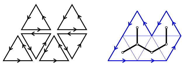
Figure 1. The diagram $D$ on the left, and the triangulated $(\lvert{T}\rvert+2)$–gon on the right, with dual graph $T$. Each triangle with corners labeled $i,j,k$ represents the vertex group $F_{i}\times F_{j}\times F_{k}$ or $G_{i}\times G_{j}\times G_{k}$. The side pairings depict the amalgamations $A_{1}=_{\tau}A_{5}$, $A_{3}=_{\tau}A_{11}$, $A_{4}=_{\tau}A_{8}$, $A_{10}=_{\tau}A_{12}$, and $A_{14}=_{\tau}A_{17}$ (in the case of $V_{T}$).

It may be helpful to consider the diagram $D$ as shown in Figure 1. It has a triangle for each vertex of $T$, with corners corresponding to the factors $F_{i}$ or $G_{i}$ of the vertex group there. The edges correspond to peripheral subgroups, and the edge-pairings between triangles correspond to amalgamations. The triangles assemble into a triangulated $(\lvert{T}\rvert+2)$–gon with dual graph $T$. (Here, $\lvert{T}\rvert$ denotes the number of vertices of $T$.)

The orientations on edges indicate the standard generating sets of the peripheral subgroups, relative to the indexing of the groups $F_{i}$ or $G_{i}$. The orientation-reversing nature of the side pairings reflects the fact that the amalgamations are performed using $\tau$.

The peripheral subgroups of $V_{T}$ (or of $W_{T}$) are defined to be the remaining peripheral subgroups of the vertex groups that were not assigned to edges of $T$. In terms of the diagram $D$, these are the peripheral subgroups corresponding to the edges forming the boundary $(\lvert{T}\rvert+2)$–gon.

Next we re-index the peripheral subgroups. Note that the boundary edges along $D$ are coherently oriented. Start with one and let $\nu_{0}$ be the index of the corresponding peripheral subgroup. Following the orientation, let $\nu_{1}$ be the index of the next edge along $\partial D$. Repeat in this way and define the indices $\nu_{0}\dotsc,\nu_{m}$, allowing us to refer to the peripheral subgroups as $A_{\nu_{0}},\dotsc,A_{\nu_{m}}$ (or $B_{\nu_{0}},\dotsc,B_{\nu_{m}}$). Note, $m=\lvert{T}\rvert+1$.

The groups $S_{T,n}$ and $G_{T,n}$

Fix a tree $T$ as above and let $m=\lvert{T}\rvert+1$. The group $S_{T,n}$ is defined to be a multiple HNN extension over $V_{T}$ with stable letters $r_{1},\dotsc,r_{m}$, where $r_{i}$ conjugates the peripheral subgroup $A_{\nu_{0}}$ to $A_{\nu_{i}}$ via the automorphism $\varphi^{n}$. That is,

$$S_{T,n}=\langle\,V_{T},r_{1},\dotsc,r_{m}\mid\ r_{i}a_{\nu_{0}}r_{i}^{-1}=\varphi^{n}(a_{\nu_{i}}),$$

$$r_{i}b_{\nu_{0}}r_{i}^{-1}=\varphi^{n}(b_{\nu_{i}})\text{ for each }i\,\rangle.$$ (3.1)

Thus $S_{T,n}$ is the fundamental group of a graph of groups whose underlying graph is the $m$–rose (having one vertex and $m$ loops). The vertex group is $V_{T}$ and the edge groups are all $F$.

We define $G_{T,n}$ in a similar manner, but without twisting. It is a multiple HNN extension over $W_{T}$ with stable letters $s_{1},\dotsc,s_{m}$, where $s_{i}$ conjugates $B_{\nu_{0}}$ to $B_{\nu_{i}}$ via the identity map:

$$G_{T,n}=\langle\,W_{T},s_{1},\dotsc,s_{m}\mid\ s_{i}a_{\nu_{0}}s_{i}^{-1}=a_{\nu_{i}},$$

$$s_{i}b_{\nu_{0}}s_{i}^{-1}=b_{\nu_{i}},\,s_{i}{c}_{\nu_{0}}s_{i}^{-1}={c}_{\nu_{i}}\text{ for each }i\,\rangle.$$ (3.2)

Again, $G_{T,n}$ is the fundamental group of a graph of groups over the $m$–rose. The vertex group is $W_{T}$ and the edge groups are all $G$.

4. The CAT(0) structure

In this section we build the CAT(0) structure for the group $G_{T,n}$.

The space $Z$

Recall that we have chosen a specific monotone palindromic automorphism $\varphi\colon\thinspace F\to F$ given by $\varphi(x)=xyx$, $\varphi(y)=x$. Let

$$G_{0}\ =\ \langle x,y\rangle\rtimes_{\varphi}\langle{t_{0}}\rangle\ =\ \langle\,x,y,{t_{0}}\mid{t_{0}}x{t_{0}}^{-1}=xyx,\ {t_{0}}y{t_{0}}^{-1}=x\,\rangle.$$ (4.1)

T. Brady [Bra95] has constructed a piecewise Euclidean, locally CAT(0) $2$–complex $Z_{0}$ with fundamental group $G_{0}$. This $2$–complex has two vertices, four edges, and two $2$–cells, consisting of a Euclidean octagon and quadrilateral as shown in Figure 2. The angle $\alpha\in(0,\pi)$ is a free parameter, and the rest of the geometry (up to scaling) is then determined. It is easy to check that both vertices satisfy the link condition, making $Z_{0}$ locally CAT(0).

2pt $\tau_{Z_{0}}$ [r] at 31 6 $\tau_{Z_{0}}$ [r] at 130 38

${\color[rgb]{0.21484375,0.73828125,0.3828125}\alpha}$ [Bl] at 46 122 ${\color[rgb]{0.21484375,0.73828125,0.3828125}\alpha}$ [Bl] at 144 86 ${\color[rgb]{0.21484375,0.73828125,0.3828125}\alpha}$ [tl] at 145 51.5 ${\color[rgb]{0.21484375,0.73828125,0.3828125}\alpha}$ [tl] at 47 18 ${\color[rgb]{0.21484375,0.73828125,0.3828125}\pi}$ [l] at 16.5 68 ${\color[rgb]{0.21484375,0.73828125,0.3828125}\pi}$ [r] at 65 68

$z_{0}$ [r] at 6 31 $z_{0}$ [l] at 74.5 31 $z_{0}$ [r] at 6 104 $z_{0}$ [l] at 74.5 104

${\color[rgb]{0,0,0.8671875}x}$ [tl] at 43.5 101.5 ${\color[rgb]{0,0,0.8671875}y}$ [Bl] at 43 38.5 ${\color[rgb]{0,0,0.8671875}t_{0}}$ [l] at 141.5 68

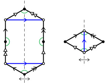
Figure 2. The piecewise Euclidean $2$–complex $Z_{0}$ and its isometric involution $\tau_{Z_{0}}$.

The figure also shows three arcs crossing the interiors of the $2$–cells, representing the elements $x$, $y$, and ${t_{0}}$ in $\pi_{1}(Z_{0},z_{0})$; we leave it to the reader to verify that $\pi_{1}(Z_{0},z_{0})$ indeed has the presentation (4.1) relative to these generators.

Reflection of each $2$–cell across the vertical dotted lines in Figure 2 respects the edge identifications, and induces an isometric involution $\tau_{Z_{0}}\colon\thinspace Z_{0}\to Z_{0}$. The induced homomorphism $\tau_{G_{0}}\colon\thinspace G_{0}\to G_{0}$ is given by $\tau_{G_{0}}(x)=\overline{x}$, $\tau_{G_{0}}(y)=\overline{y}$, and $\tau_{G_{0}}({t_{0}})={t_{0}}$.

Let $t=(t_{0})^{n}$ and note that the index-$n$ subgroup $\langle x,y,t\rangle\triangleleft G_{0}$ is the group $G$ defined earlier. The corresponding covering space $Z$ of $Z_{0}$ has a locally CAT(0) structure made from $n$ octagons and $n$ quadrilaterals. The involution $\tau_{Z_{0}}$ lifts to an isometric involution $\tau_{Z}\colon\thinspace Z\to Z$, with induced homomorphism $\tau_{G}$. The case $n=3$ is shown in Figure 3.

2pt $\tau_{Z}$ [r] at 11 75 $\tau_{Z}$ [r] at 65 93 $\tau_{Z}$ [r] at 119 40 $\tau_{Z}$ [r] at 173 57 $\tau_{Z}$ [r] at 227 4 $\tau_{Z}$ [r] at 281 21

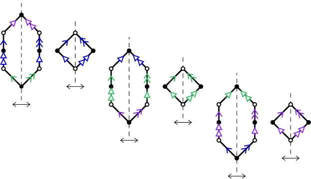
Figure 3. The locally CAT(0) $2$–complex $Z$ and its involution $\tau_{Z}$, when $n=3$.

To summarize, we now have a locally CAT(0) space $Z$ with fundamental group $G$, and an isometric involution $\tau_{Z}\colon\thinspace Z\to Z$ whose induced homomorphism is given by the involution $\tau_{G}$.

The space $K_{T}$

We shall need the following “gluing with a tube” result.

Proposition 4.2 ([BH99], II.11.13).

Let $X$ and $A$ be locally CAT(0) metric spaces. If $A$ is compact and $\varphi,\psi\colon\thinspace A\to X$ are locally isometric immersions, then the quotient of $X\sqcup(A\times[0,1])$ by the equivalence relation generated by $(a,0)\sim\varphi(a);(a,1)\sim\psi(a)$, $\forall a\in A$ is locally CAT(0).

Let $Z_{i}$ and $Z_{j}$ be copies of $Z$ with fundamental groups $G_{i}$ and $G_{j}$ repsectively. Let $Z_{i}\times Z_{j}$ be given the product metric. Define the map $f_{i,j}\colon\thinspace Z\to Z_{i}\times Z_{j}$ by $f_{i,j}(p)=(\tau_{z}(p),p)$. Note that the induced homomorphism $(f_{i,j})_{*}\colon\thinspace G\to G_{i}\times G_{j}$ is given by $x\mapsto\overline{x}_{i}x_{j}$, $y\mapsto\overline{y}_{i}y_{j}$, $t\mapsto t_{i}t_{j}$. Metrically, $f_{i,j}$ behaves as follows:

$$d(f_{i,j}(p),f_{i,j}(q))\ =\ d((\tau_{Z}(p),p),(\tau_{Z}(q),q))$$

$$=\ (d(\tau_{Z}(p),\tau_{Z}(q))^{2}+d(p,q)^{2})^{1/2}$$

$$=\ (2d(p,q)^{2})^{1/2}\ =\ \sqrt{2}d(p,q).$$

Hence $f_{i,j}$ is an isometric embedding of the scaled metric space $(\sqrt{2})Z$ into $Z_{i}\times Z_{j}$.

Now we define the locally CAT(0) space $K_{T}$ with fundamental group $W_{T}$. Let

$$K=Z_{0}\times Z_{1}\times Z_{2}$$

where each $Z_{i}$ is a copy of $Z$. Thus, $K$ is locally CAT(0) and has fundamental group $W=G_{0}\times G_{1}\times G_{2}$. Fix a basepoint $v\in Z$ and let $v_{i}\in Z_{i}$ be the corresponding points. Each product space $Z_{i}\times Z_{i+1}$ isometrically embeds into $K$ using the basepoint $v_{i-1}$ as the missing coordinate (indices mod $3$). Define the peripheral subspace $L_{i}$ to be the image of the map

$$Z\ \overset{f_{i,i+1}}{\longrightarrow}\ Z_{i}\times Z_{i+1}\ \hookrightarrow\ K.$$ (4.3)

Note that $L_{i}$ has fundamental group $B_{i}<W$ and the induced map $\pi_{1}(Z,v)\to W$ is the standard inclusion map $x\mapsto a_{i}$, $y\mapsto b_{i}$, $t\mapsto c_{i}$ with image $B_{i}$.

The space $K_{T}$ is formed from copies of $K$ in the same way that $W_{T}$ is built from copies of $W$. Take a copy of $K$ for each vertex of $T$, with all indices re-named to agree with the triple of indices assigned to that vertex. Whenever $B_{i}$ and $B_{j}$ were amalgamated in $W_{T}$, glue the ends of a tube $(\sqrt{2})Z\times[0,1]$ to the peripheral subspaces $L_{i}$ and $L_{j}$, using the isometric embedding (4.3) from $(\sqrt{2})Z\times\{0\}$ to the copy of $K$ containing $L_{i}$, and using a similar isometric embedding

$$Z\overset{\tau_{Z}}{\longrightarrow}\ Z\ \overset{f_{j,j+1}}{\longrightarrow}\ Z_{j}\times Z_{j+1}\ \hookrightarrow\ K$$

from $(\sqrt{2})Z\times\{1\}$ to the copy of $K$ containing $L_{j}$. The involution $\tau_{Z}$ is being used to obtain the correct identification between the subgroups $B_{i}$ and $B_{j}$. The resulting space $K_{T}$ has fundamental group $W_{T}$, and is locally CAT(0) by Proposition 4.2. In particular, $W_{T}$ is CAT(0).

Remark 4.4.

The reasoning above also shows that $V_{T}$ is CAT(0). One simply re-defines $Z$ to be the space $S^{1}\vee S^{1}$ with any path metric (which will be locally CAT(0)). There is an obvious isometric involution $\tau_{Z}$ which reverses the direction of each loop in $Z$, and induces $\tau_{F}\colon\thinspace F\to F$. The rest is entirely similar.

The space $K_{T,n}$

Inside $K_{T}$ there are peripheral subspaces $L_{\nu_{0}},\dotsc,L_{\nu_{m}}$. For each $j=1,\dotsc,m$ glue the ends of a tube $(\sqrt{2})Z\times[0,1]$ to $L_{\nu_{0}}$ and $L_{\nu_{j}}$ using the isometric embeddings (4.3) from $(\sqrt{2})Z\times\{0\}$ and $(\sqrt{2})Z\times\{1\}$ to the appropriate copies of $K$ in $K_{T}$. The resulting space $K_{T,n}$ is the total space of a graph of spaces corresponding to the description (3) of $G_{T,n}$ as the fundamental group of a graph of groups. In particular, $K_{T,n}$ has fundamental group $G_{T,n}$. It is locally CAT(0) by Proposition 4.2. Thus we have proved:

Theorem 4.5.

$G_{T,n}$ is CAT(0). ∎

5. Embedding results

In this section we define the embedding $S_{T,n}\to G_{T,n}$ and prove that it is injective. The map is defined step by step, following the constructions defining $S_{T,n}$ and $G_{T,n}$. In several places we use the following lemma to establish injectivity. It is a special case of a basic result of Bass [Bas93], reformulated slightly.

Lemma 5.1 (Injectivity for graphs of groups).

Suppose $\mathscr{A}$ and $\mathscr{B}$ are graphs of groups such that the underlying graph $\Gamma_{\mathscr{A}}$ of $\mathscr{A}$ is a subgraph of the underlying graph of $\mathscr{B}$. Let $A$ and $B$ be their respective fundamental groups. Suppose that there are injective homomorphisms $\psi_{e}\colon\thinspace A_{e}\to B_{e}$ and $\psi_{v}\colon\thinspace A_{v}\to B_{v}$ between edge and vertex groups, for all edges $e$ and vertices $v$ in $\Gamma_{\mathscr{A}}$, which are compatible with the edge-inclusion maps.

(That is, whenever $e$ has initial vertex $v$, the diagram

$$\begin{CD}A_{e}@>{}>{}>A_{v}\\ @V{\psi_{e}}V{}V@V{\psi_{v}}V{}V\\ B_{e}@>{}>{}>B_{v}\end{CD}$$

commutes.)

If $\psi_{e}(A_{e})=\psi_{v}(A_{v})\cap B_{e}$ whenever $e$ has initial vertex $v$, then the induced homomorphism $\psi\colon\thinspace A\to B$ is injective.

Remark 5.2.

Given the initial assumptions, it is always true that $\psi_{e}(A_{e})\subset(\psi_{v}(A_{v})\cap B_{e})$. In practice one only needs to verify that $\psi_{e}(A_{e})$ contains $\psi_{v}(A_{v})\cap B_{e}$.

Proof.

The homomorphisms $\psi_{e}$, $\psi_{v}$ combine to give a morphism of graphs of groups in the sense of Bass [Bas93]. According to Proposition 2.7 of [Bas93], $\psi\colon\thinspace A\to B$ will be injective if, whenever $e$ has initial vertex $v$, the function $A_{v}/A_{e}\to B_{v}/B_{e}$ induced by $\psi_{v}$ is injective.

To prove that the latter statement holds, suppose that the cosets $\psi_{v}(a_{1})B_{e}$ and $\psi_{v}(a_{2})B_{e}$ are equal for some $a_{1},a_{2}\in A_{v}$. Then $\psi_{v}(a_{1}a_{2}^{-1})\in B_{e}$, and hence (by the main assumption) $\psi_{v}(a_{1}a_{2}^{-1})\in\psi_{e}(A_{e})$. Since $\psi_{e}$ is injective (and agrees with $\psi_{v}$), $a_{1}a_{2}^{-1}\in A_{e}$, and therefore $a_{1}A_{e}=a_{2}A_{e}$. ∎

Lemma 5.3.

Let $\iota\colon\thinspace V\to W$ be inclusion. Then $\iota(A_{i})=\iota(V)\cap B_{i}$ for each $i$.

Proof.

Without loss of generality let $i=0$. Note that $\iota(A_{0})$ and $\iota(V)\cap{B}_{0}$ are both contained in the subgroup ${G}_{0}\times{G}_{1}$, so it suffices to show that $\iota(A_{0})=\iota(F_{0}\times F_{1})\cap{B}_{0}$ in ${G}_{0}\times{G}_{1}$. One direction, $\iota(A_{0})\subset\iota(F_{0}\times F_{1})\cap{B}_{0}$, is obvious.

For the other direction, consider an element of $\iota(F_{0}\times F_{1})\cap B_{0}$. It can be expressed as a word $w(\overline{x}_{0}x_{1},\overline{y}_{0}y_{1},t_{0}t_{1})$, which equals $w(\overline{x}_{0},\overline{y}_{0},t_{0})w(x_{1},y_{1},t_{1})$ in $G_{0}\times G_{1}$. Being in $\iota(F_{0}\times F_{1})$ it also has an expression of the form $u(\overline{x}_{0},\overline{y}_{0})v(x_{1},y_{1})$ where $u$ and $v$ are reduced words in the free group. Projecting onto the second factor of $G_{0}\times G_{1}$, one obtains the equation in $G$:

$$w(x,y,t)=v(x,y).$$

Considering $G$ as an HNN extension with vertex group $F$ and stable letter $t$, the right hand side is a word in normal form (that is, a word of length $1$ consisting of an element of $F$), and therefore gives the (unique) normal form representative for the element $w$. Similarly, considering $\{\overline{x}_{0},\overline{y}_{0}\}$ as a basis for $F_{0}$, projecting onto the first factor gives the equation in $G$

$$w(x,y,t)=u(x,y)$$

and hence $u(x,y)$ is also the normal form for $w$. We conclude that $u$ and $v$ represent the same element of $F$. Since both words are reduced, they are equal as words and so $u(\overline{x}_{0},\overline{y}_{0})v(x_{1},y_{1})=u(\overline{x}_{0},\overline{y}_{0})u(x_{1},y_{1})=u(\overline{x}_{0}x_{1},\overline{y}_{0}y_{1})\in\iota(A_{0})$. ∎

Proposition 5.4.

The inclusion maps $F_{i}\hookrightarrow G_{i}$ induce an injective homomorphism $V_{T}\to W_{T}$.

Henceforth we will regard $V_{T}$ as a subgroup of $W_{T}$.

Proof.

We will use Lemma 5.1 since $V_{T}$ and $W_{T}$ are both fundamental groups of graphs of groups with underlying graph $T$.

To elaborate on the graph of groups structures of $V_{T}$ and $W_{T}$, fix an orientation of each edge of $T$ and use these to specify the edge-inclusion maps as follows. For $V_{T}$, each edge group is $F$ and the two neighboring vertex groups are isomorphic to $V$. For the initial vertex, the inclusion map $F\to F_{i}\times F_{i+1}$ is $\tau_{F}\times\operatorname{id}$, and for the terminal vertex, the inclusion map $F\to F_{j}\times F_{j+1}$ is $\operatorname{id}\times\tau_{F}$. In the case of $W_{T}$, the same convention is used: inclusion maps $G\to G_{i}\times G_{i+1}$ are $\tau_{G}\times\operatorname{id}$ for initial vertices and $\operatorname{id}\times\tau_{G}$ for terminal vertices.

The inclusion maps $F_{i}\to G_{i}$ induce inclusions between corresponding vertex groups $V\to W$. The compatibility diagrams become

$$\begin{CD}F@>{\tau_{F}\times\operatorname{id}}>{}>F_{i}\times F_{i+1}@>{}>{}>V\\ @V{}V{}V&&@V{}V{}V\\ G@>{\tau_{G}\times\operatorname{id}}>{}>G_{i}\times G_{i+1}@>{}>{}>W\end{CD}\ \ \text{or}\ \ \begin{CD}F@>{\operatorname{id}\times\tau_{F}}>{}>F_{i}\times F_{i+1}@>{}>{}>V\\ @V{}V{}V&&@V{}V{}V\\ G@>{\operatorname{id}\times\tau_{G}}>{}>G_{i}\times G_{i+1}@>{}>{}>W\end{CD}$$

and these clearly commute (all unnamed maps are inclusion). Thus there is an induced homomorphism $V_{T}\to W_{T}$. The last condition needed by Lemma 5.1 is provided by Lemma 5.3, and so we conclude from 5.1 that $V_{T}\to W_{T}$ is injective. ∎

Change of coordinates in $G_{T,n}$

We plan to use Lemma 5.1 to embed $S_{T,n}$ into $G_{T,n}$, but first we must modify the graph of groups structure of $G_{T,n}$. The modification amounts to a change in the choice of stable letters in the multiple HNN extension description of $G_{T,n}$. Alternatively, it can be seen as an application of Tietze transformations.

Indeed, one can start with the presentation (3) defining $G_{T,n}$, add new generators $u_{1},\dotsc,u_{m}$ and relations $u_{i}={c}_{\nu_{i}}s_{i}$, replace occurrences of $s_{i}$ with ${c}_{\nu_{i}}^{-1}u_{i}$, and delete the generators $s_{i}$. The relation $s_{i}a_{\nu_{0}}s_{i}^{-1}=a_{\nu_{i}}$ becomes ${c}_{\nu_{i}}^{-1}u_{i}a_{\nu_{0}}u_{i}^{-1}{c}_{\nu_{i}}=a_{\nu_{i}}$, or equivalently, $u_{i}a_{\nu_{0}}u_{i}^{-1}={c}_{\nu_{i}}a_{\nu_{i}}{c}_{\nu_{i}}^{-1}=\varphi^{n}(a_{\nu_{i}})$. Similarly, the relation $s_{i}b_{\nu_{0}}s_{i}^{-1}=b_{\nu_{i}}$ becomes $u_{i}b_{\nu_{0}}u_{i}^{-1}=\varphi^{n}(b_{\nu_{i}})$ and the relation $s_{i}{c}_{\nu_{0}}s_{i}^{-1}={c}_{\nu_{i}}$ becomes $u_{i}{c}_{\nu_{0}}u_{i}^{-1}={c}_{\nu_{i}}$. Thus one obtains the new presentation

$$G_{T,n}=\langle\,W_{T},u_{1},\dotsc,u_{m}\mid\ u_{i}a_{\nu_{0}}u_{i}^{-1}=\varphi^{n}(a_{\nu_{i}}),\,$$

$$u_{i}b_{\nu_{0}}u_{i}^{-1}=\varphi^{n}(b_{\nu_{i}}),\,u_{i}{c}_{\nu_{0}}u_{i}^{-1}={c}_{\nu_{i}}\text{ for each }i\,\rangle.$$ (5.5)

This is evidently the presentation arising from a new description of $G_{T,n}$ as a multiple HNN extension of $W_{T}$ with stable letters $u_{1},\dotsc,u_{m}$, where $u_{i}$ conjugates $B_{\nu_{0}}$ to $B_{\nu_{i}}$ via $\varphi^{n}\times\operatorname{id}$.

Theorem 5.6.

The homomorphism $S_{T,n}\to G_{T,n}$ induced by the inclusion $V_{T}\hookrightarrow W_{T}$ and the assigment $r_{i}\mapsto u_{i}$ is injective.

Proof.

First, given the presentations (3) and (5), it is clear that the given assignment defines a homomorphism $S_{T,n}\to G_{T,n}$. Furthermore, this is the homomorphism induced by the injective maps on vertex and edge groups: $V_{T}\hookrightarrow W_{T}$ in the case of the vertex, and $F\hookrightarrow G$ for each edge of the $m$–rose. The corresponding compatibility diagrams are

$$\begin{CD}F@>{\operatorname{id}}>{}>A_{\nu_{0}}@>{}>{}>V_{T}\\ @V{}V{}V&&@V{}V{}V\\ G@>{\operatorname{id}}>{}>B_{\nu_{0}}@>{}>{}>W_{T}\end{CD}\ \ \ \ \text{and}\ \ \ \ \begin{CD}F@>{\varphi^{n}}>{}>A_{\nu_{i}}@>{}>{}>V_{T}\\ @V{}V{}V&&@V{}V{}V\\ G@>{\varphi^{n}\times\operatorname{id}}>{}>B_{\nu_{i}}@>{}>{}>W_{T}\end{CD}$$

where $A_{j}$ and $B_{j}$ are canonically identified with $F$ and $G$ via their standard generating sets, and the unnamed maps are inclusion. These diagrams commute.

We have all of the initial hypotheses of Lemma 5.1 satisfied. It remains to verify that $A_{\nu_{i}}=V_{T}\cap B_{\nu_{i}}$ in $W_{T}$ for $i=0,\dotsc,m$. Consider the vertex of $T$ whose triple of indices includes $\nu_{i}$. Let $V$ and $W$ be the vertex groups at that vertex (for the graph of groups decompositions of $V_{T}$ and $W_{T}$). Then $A_{\nu_{i}}$ and $V_{T}\cap B_{\nu_{i}}$ are both contained in $W$. Moreover $W\cap V_{T}=V$, and so it suffices to show that $A_{\nu_{i}}=V\cap B_{\nu_{i}}$. This holds by Lemma 5.3. Hence, by Lemma 5.1, the map $S_{T,n}\to G_{T,n}$ is injective. ∎

6. Corridor schemes and the balancing property of $V_{T}$

In this section we develop two key tools which will play an essential role throughout the rest of the paper. These tools are specific to the groups $V_{T}$, and they are the primary means by which we establish the various properties of $V_{T}$ that are needed. The first of these is the notion of $\sigma$–corridors in van Kampen diagrams over $V_{T}$. The second is the balancing property of $V_{T}$, given in Proposition 6.7.

In order to discuss $\sigma$–corridors we first define corridor schemes. We will make use of several corridor schemes in this paper, in addition to $\sigma$–corridors. In this section we also discuss the standard generating set for $V_{T}$, and various notions of length associated with this generating set.

The $2$–complex $X_{T}$

In order to discuss area in $V_{T}$ we will work with a specific $2$–complex $X_{T}$ with fundamental group $V_{T}$.

The group $V$ has a presentation with generators $x_{i},y_{i},a_{i},b_{i}$ for $i=0,1,2$ and eighteen relations (see also Figure 5):

$$a_{i}=\overline{x}_{i}x_{i+1},\ \ a_{i}=x_{i+1}\overline{x}_{i},\ \ b_{i}=\overline{y}_{i}y_{i+1},\ \ b_{i}=y_{i+1}\overline{y}_{i},$$

$$x_{i}y_{i+1}=y_{i+1}x_{i},\ \ x_{i+1}y_{i}=y_{i}x_{i+1}\ \ (i=0,1,2\mod 3)$$ (6.1)

We define $X$ to be the presentation $2$–complex for this presentation of $V$. Thus $X$ has one $0$–cell, twelve labeled, oriented $1$–cells, twelve triangular $2$–cells, and six quadrilateral $2$–cells.

For each $i$, the subcomplex $Y_{i}\subset X$ consisting of the two $1$–cells labeled $a_{i}$ and $b_{i}$ is called a peripheral subspace. It is homeomorphic to $S^{1}\vee S^{1}$ and has fundamental group $A_{i}\subset V$.

The $2$–complex $X_{T}$ is formed from copies of $X$ in the same way that $V_{T}$ is built from copies of $V$. Take a copy of $X$ for each vertex of $T$, with edge labels re-indexed according to the triple of indices assigned to that vertex. Whenever $A_{i}$ and $A_{j}$ were amalgamated in $V_{T}$, glue the peripheral subspaces $Y_{i}$ and $Y_{j}$ via a cellular homeomorphism which induces $\tau$ between $A_{i}$ and $A_{j}$. The resulting space $X_{T}$, with fundamental group $V_{T}$, has a natural cell structure. The $1$–cells are labeled by the generators $x_{i}$, $y_{i}$, $a_{i}$, and $b_{i}$, where in some cases, a $1$–cell labeled $a_{i}$ or $b_{i}$ is also labeled $a_{j}$ or $b_{j}$ in the opposite direction. The $2$–cells are the same as those of the copies of $X$, with the same triangular and quadrilateral boundary relations.

Area

In order to simplify the area calculations to follow, we declare each triangular cell of $X_{T}$ to have area $1$, and each quadrilateral cell to have area $2$. (Think of it as being made of two triangles.)

Corridor schemes

Let $Z$ be any presentation $2$–complex. A corridor scheme for $Z$ is a subset ${{\mathscr{S}}}$ of the set of edges of $Z$ such that every $2$–cell of $Z$ has either zero or two occurrences of edges of ${{\mathscr{S}}}$ in its boundary. Given such an ${{\mathscr{S}}}$, one can then define corridors in any van Kampen diagram over $Z$. Call the $2$–cells having two ${{\mathscr{S}}}$–edges in their boundaries corridor cells. Given a van Kampen diagram $\Delta$, two corridor cells in $\Delta$ are called neighbors if they meet along an ${{\mathscr{S}}}$–edge in their boundaries. A corridor cell has zero, one, or two neighbors. A corridor is a minimal collection $C$ of corridor cells in $\Delta$ such that if $c\in C$ then all neighbors of $c$ are also in $C$. Every corridor cell is contained in a corridor.

Corridors come in two types: those in which every corridor cell has neighbors along both of its ${{\mathscr{S}}}$–edges, called annulus type, and the others, called band type. Each band type corridor joins an ${{\mathscr{S}}}$–edge on the boundary of $\Delta$ to another ${{\mathscr{S}}}$–edge on the boundary of $\Delta$, and contains no other ${{\mathscr{S}}}$–edges on the boundary of $\Delta$. An annulus type corridor may have $2$–cells meeting the boundary of $\Delta$, but the ${{\mathscr{S}}}$–edges of such $2$–cells will not be on the boundary.

If $C$ is a corridor in $\Delta$, then the subset formed by taking the union of the interiors of its $2$–cells along with the interiors of its ${{\mathscr{S}}}$–edges is an open set, homeomorphic to a tubular neighborhood of a properly embedded connected $1$–dimensional submanifold of $\Delta$. The $1$–manifold meets each corridor cell in an arc joining the two ${{\mathscr{S}}}$–edges of the cell. Thus an annulus type corridor contains an embedded open annulus, and a band type corridor contains an embedded open band $[0,1]\times(0,1)$ meeting the boundary of the diagram in its boundary $\{0,1\}\times(0,1)$.

Corridors have two key properties. First, two corridors in a diagram $\Delta$ will never have $2$–cells or ${{\mathscr{S}}}$–edges in common. In particular, corridors cannot cross. Second, every ${{\mathscr{S}}}$–edge appearing on the boundary of $\Delta$ is part of a band type corridor, unless that edge is not in any $2$–cell of $\Delta$. In particular, given an ${{\mathscr{S}}}$–edge in the boundary of $\Delta$, if there is a $2$–cell containing that edge, then one can pass from neighbor to neighbor in the corridor, until one arrives at a second, uniquely determined, ${{\mathscr{S}}}$–edge on the boundary of $\Delta$. Also, in the boundary, this pair of ${{\mathscr{S}}}$–edges cannot be linked with another such pair, because corridors do not cross.

Orientable corridor schemes

A corridor scheme ${{\mathscr{S}}}$ is orientable if there is a choice of orientations of the edges of ${{\mathscr{S}}}$ such that in each corridor cell, the two ${{\mathscr{S}}}$–edges have oppposite orientations relative to the boundary of the cell. It follows that in any corridor, the transverse orientations of the ${{\mathscr{S}}}$–edges along the corridor all agree.

Remark 6.2.

A corridor scheme defines a $1$–dimensional ${\mathbb{Z}}_{2}$–valued cellular cocycle in $Z$. (If $Z$ happens to be a simplicial complex, then every $1$–cocycle is a corridor scheme.) An orientable corridor scheme defines a ${\mathbb{Z}}$–valued $1$–cocycle in $Z$. See Gersten [Ger98] for a thorough study of corridors from the cohomological point of view.

${\sigma}$–corridors

Recall that $D$ was a diagram made of triangles, with dual graph $T$, which may be regarded as being embedded as a subspace of a triangulated $(\lvert{T}\rvert+2)$–gon. Let $\widehat{T}$ be a tree obtained from $T$ by joining the midpoint of each boundary edge to the vertex in the neighboring triangle. Then $\widehat{T}$ has $m+1$ leaves, corresponding to the peripheral subgroups of $V_{T}$, and interior vertices all of valence three, which are the original vertices of $T$. Denote the leaves of $\widehat{T}$ by $v_{\nu_{0}},\dotsc,v_{\nu_{m}}$, so that $v_{\nu_{i}}$ corresponds to the peripheral subgroup $A_{\nu_{i}}$.

Let ${\sigma}$ be a maximal segment in $\widehat{T}$. Note that ${\sigma}$ is uniquely determined by its endpoints; choosing ${\sigma}$ amounts to choosing a pair of peripheral subgroups of $V_{T}$. For each such ${\sigma}$ we will define a corridor scheme ${{\mathscr{S}}}_{{\sigma}}$ for $X_{T}$.

In the $(\lvert{T}\rvert+2)$–gon, ${\sigma}$ starts on a boundary edge, passes through a sequence of triangles, and ends on a boundary edge. Its intersection with each of these triangles is an arc joining two sides. It separates one corner of the triangle from the other two. If $i$ is the index of this corner, put the edges of $X_{T}$ labeled by $x_{i}$ and $y_{i}$ into ${{\mathscr{S}}}_{{\sigma}}$. Also, if ${\sigma}$ passes through the side of a triangle associated with the subgroup $A_{j}$, put the edges labeled by $a_{j}$ and $b_{j}$ into ${{\mathscr{S}}}_{{\sigma}}$. Do this for each triangle that intersects ${\sigma}$ to obtain ${{\mathscr{S}}}_{{\sigma}}$. The fact that some edges of $X_{T}$ have two labels is not a problem; either both labels or neither label will be chosen for inclusion in ${{\mathscr{S}}}_{{\sigma}}$. See Figure 4.

2pt ${\color[rgb]{0.21484375,0.73828125,0.3828125}\sigma}$ [tr] at 30 7 ${\color[rgb]{0.21484375,0.73828125,0.3828125}\sigma}$ [Bl] at 82 79

* ${\color[rgb]{0,0,1}0}$ at 17 20 * ${\color[rgb]{0,0,1}1}$ at 48 20 * ${\color[rgb]{0,0,1}2}$ at 32.5 47 * ${\color[rgb]{0,0,1}3}$ at 79.5 38 * ${\color[rgb]{0,0,1}4}$ at 95 65 * ${\color[rgb]{0,0,1}5}$ at 63 65

$A_{1}$ [Bl] at 40 52 $A_{5}$ [tr] at 73 36 $A_{3}$ [tl] at 102 63 $A_{4}$ [Br] at 71 78 $A_{2}$ [Br] at 9.5 27 $A_{0}$ [tl] at 41 9

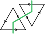
Figure 4. This portion of ${\sigma}$ passing through $D$ contributes the following edges of $X_{T}$ to ${{\mathscr{S}}}_{{\sigma}}$: $a_{0}$, $b_{0}$, $x_{1}$, $y_{1}$, $a_{1}$ ($=a_{5}$), $b_{1}$ ($=b_{5}$), $x_{5}$, $y_{5}$, $a_{4}$, $b_{4}$.

One verifies easily that ${{\mathscr{S}}}_{{\sigma}}$ is a corridor scheme, by examining the relations (6.1) for each triangle of $D$. See also Figure 5. (Because of the two-label phenomenon, it is important here that ${\sigma}$ is maximal.) Corridors defined by this scheme will be called ${\sigma}$–corridors.

2pt $x_{0}$ [b] at 12 100.5 $x_{0}$ [b] at 53 100.5 $x_{1}$ [b] at 93 100.5 $x_{1}$ [b] at 133 100.5 $x_{2}$ [b] at 174 100.5 $x_{2}$ [b] at 214 100.5

$y_{1}$ [r] at 2 90.5 $y_{1}$ [l] at 22.5 90.5 $y_{2}$ [r] at 42 90.5 $y_{2}$ [l] at 63 90.5 $y_{0}$ [r] at 82.5 90.5 $y_{0}$ [l] at 103.5 90.5 $y_{2}$ [r] at 123 90.5 $y_{2}$ [l] at 144 90.5 $y_{0}$ [r] at 163.5 90.5 $y_{0}$ [l] at 184.5 90.5 $y_{1}$ [r] at 204.5 90.5 $y_{1}$ [l] at 225 90.

$x_{0}$ [t] at 12 79.5 $x_{0}$ [t] at 53 79.5 $x_{1}$ [t] at 93 79.5 $x_{1}$ [t] at 133 79.5 $x_{2}$ [t] at 174 79.5 $x_{2}$ [t] at 214 79.5

$x_{0}$ [b] at 50 64.5 $x_{1}$ [b] at 122 64.5 $x_{2}$ [b] at 194 64.5

* $a_{0}$ at 40.5 54 * $a_{1}$ at 113 54 * $a_{2}$ at 184.5 54

$x_{1}$ [r] at 21 54 $x_{1}$ [l] at 61 54 $x_{2}$ [r] at 93 54 $x_{2}$ [l] at 133 54 $x_{0}$ [r] at 165 54 $x_{0}$ [l] at 205 54

$x_{0}$ [t] at 32 43.5 $x_{1}$ [t] at 104 43.5 $x_{2}$ [t] at 177 43.5

$y_{0}$ [b] at 50 28.5 $y_{1}$ [b] at 122 28.5 $y_{2}$ [b] at 194 28.5

$y_{1}$ [r] at 21 18.5 $y_{1}$ [l] at 61 18.5 $y_{2}$ [r] at 93 18.5 $y_{2}$ [l] at 133 18.5 $y_{0}$ [r] at 165 18.5 $y_{0}$ [l] at 205 18.5

* $b_{0}$ at 41 18.5 * $b_{1}$ at 113.5 18.5 * $b_{2}$ at 185.5 18.5

$y_{0}$ [t] at 32 7 $y_{1}$ [t] at 104 7 $y_{2}$ [t] at 177 7

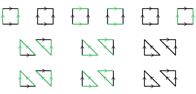
Figure 5. Part of the corridor scheme ${{\mathscr{S}}}_{{\sigma}}$, in green, for the segment ${\sigma}$ from Figure 4. The $2$–cells from the copy of $X$ with triple $(0,1,2)$ are shown. There is an analogous collection of corridor cells for every triangle that $\sigma$ meets.

Remark 6.3.

Looking closely at the corridor scheme ${{\mathscr{S}}}_{{\sigma}}$, two additional properties become evident. First, the ${{\mathscr{S}}}_{{\sigma}}$–edges appearing in a single corridor are all labeled $x_{i}$ or $a_{i}$ for various indices $i$, or they are all labeled $y_{i}$ or $b_{i}$. (That is, ${{\mathscr{S}}}_{{\sigma}}$ is the disjoint union of two smaller corridor schemes.)

Second, the corridor scheme ${{\mathscr{S}}}_{{\sigma}}$ is orientable. Referring to Figure 5, we can give positive orientations (relative to the labeling) to the edges labeled $x_{0}$, $y_{0}$, $x_{1}$, $y_{1}$, $a_{0}$, and $b_{0}$, and negative orientations to those labeled $a_{1}$ and $b_{1}$. This set of choices, or its opposite, can be imposed on any copy of $X$ in $X_{T}$ that contains edges of ${{\mathscr{S}}}_{{\sigma}}$. If two copies are adjacent, meaning that they intersect in a subspace $Y_{i}$, then the orientations on each copy can be made to agree on $Y_{i}$, by reversing the choices on one side if necessary. Now recall that the copies of $X$ containing edges of ${{\mathscr{S}}}_{{\sigma}}$ all lie along ${\sigma}$. Starting with the copy of $X$ at one end, one may propagate these choices consistently over all of ${{\mathscr{S}}}_{{\sigma}}$.

Orientability implies that if an ${{\mathscr{S}}}_{{\sigma}}$–edge label appears more than once along a corridor, then it is oriented the same way across the corridor in each occurrence. Furthermore, if a band type corridor joins two ${{\mathscr{S}}}_{{\sigma}}$–edges in the boundary which carry the same label, then those labels have opposite orientations relative to the boundary of the diagram.

Standard generators for $V_{T}$

Recall that $V_{T}$ contains many free subgroups $A_{i}=\langle a_{i},b_{i}\rangle$ which were the peripheral subgroups of the vertex groups $V$. Some of these subgroups were assigned to edges of $T$ and amalgamated together; these subgroups of $V_{T}$ will be called the internal subgroups, and their generators the internal generators. Recall that every $A_{i}$ that is not an internal subgroup is called a peripheral subgroup of $V_{T}$.

The standard generating set for $V_{T}$ will be the union of the generators of the vertex groups (all the generators $x_{i}$ and $y_{i}$) and the generators $a_{i},b_{i}$ of the peripheral subgroups. The internal generators are not included.

Definition 6.4.

If $w$ is a word let $\lvert{w}\rvert$ denote the length of $w$. We define some additional lengths for a word $w$ in the standard generators of $V_{T}$:

• $\lvert{w}\rvert_{x}$ is the number of occurrences of letters $x_{i}^{\pm 1}$ (for any $i$) in $w$

• $\lvert{w}\rvert_{y}$ is the number of occurrences of letters $y_{i}^{\pm 1}$ (for any $i$) in $w$

• for each $i$, $\lvert{w}\rvert_{i}$ is the number of occurrences of letters $a_{i}^{\pm 1},b_{i}^{\pm 1}$ in $w$

Clearly, $\lvert{w}\rvert=\lvert{w}\rvert_{x}+\lvert{w}\rvert_{y}+\sum_{i}\lvert{w}\rvert_{i}$.

We use similar notation to count occurrences of $x^{\pm 1}$ and $y^{\pm 1}$ in words representing elements of $\langle x,y\rangle$.

Definition 6.5.

We also define weighted word lengths $\lVert{w}\rVert$ similar to the lengths above, where letters are counted with real-valued weights.

Recall that $\varphi$ has transition matrix $M_{\varphi}=\begin{pmatrix}\,\lvert{\varphi(x)}\rvert_{x}&\lvert{\varphi(y)}\rvert_{x}\\ \lvert{\varphi(x)}\rvert_{y}&\lvert{\varphi(y)}\rvert_{y}\,\end{pmatrix}$ with Perron-Frobenius eigenvalue $\lambda>1$. Let $\vec{d}$ be a left eigenvector for $\lambda$ (so that $\vec{d}M_{\varphi}=\lambda\vec{d}$) with positive entries $d_{1}$ and $d_{2}$.

To define the weighted word lengths, we assign the weight $d_{1}$ to the letters $x_{i}$ and $a_{i}$, and we assign $d_{2}$ to each $y_{i}$ and $b_{i}$. Thus,

• $\lVert{w}\rVert_{x}=d_{1}\lvert{w}\rvert_{x}$

• $\lVert{w}\rVert_{y}=d_{2}\lvert{w}\rvert_{y}$

The weighted length functions are needed for the sake of Lemma 6.6 below. Up to scaling, this is the only choice of weights for which the conclusion of the lemma holds.

Lemma 6.6.

Suppose $w$ is a word in the free group $\langle x,y\rangle$ and $v$ is the reduced word representing $\varphi(w)$. Let $\lVert{\,\cdot\,}\rVert$ denote the weighted word length which assigns weight $d_{1}$ to $x^{\pm 1}$ and weight $d_{2}$ to $y^{\pm 1}$, where $\vec{d}M_{\varphi}=\lambda\vec{d}$. Then $\lVert{v}\rVert\leqslant\lambda\lVert{w}\rVert$.

Proof.

This is a simple calculation:

$$\lVert{\varphi(w)}\rVert\ =\ d_{1}\lvert{\varphi(w)}\rvert_{x}+d_{2}\lvert{\varphi(w)}\rvert_{y}$$

$$=\ d_{1}\lvert{\varphi(x)}\rvert_{x}\lvert{w}\rvert_{x}+d_{1}\lvert{\varphi(y)}\rvert_{x}\lvert{w}\rvert_{y}+d_{2}\lvert{\varphi(x)}\rvert_{y}\lvert{w}\rvert_{x}+d_{2}\lvert{\varphi(y)}\rvert_{y}\lvert{w}\rvert_{y}$$

$$=\ \lambda d_{1}\lvert{w}\rvert_{x}+\lambda d_{2}\lvert{w}\rvert_{y}$$

$$=\ \lambda\lVert{w}\rVert.$$

Now, $\lVert{v}\rVert\leqslant\lVert{\varphi(w)}\rVert=\lambda\lVert{w}\rVert$. ∎

The balancing property

A fundamental property of $V_{T}$ and its standard generating set, the balancing property, is given in the next proposition.

Proposition 6.7.

Suppose $w$ and $z(a_{\nu_{0}},b_{\nu_{0}})$ represent the same element of $A_{\nu_{0}}\subset V_{T}$, where $w$ is a word in the standard generators of $V_{T}$ and $z(a_{\nu_{0}},b_{\nu_{0}})$ is reduced. Then for each $i=1,\dotsc,m$ there is an inequality

$$\lvert{z}\rvert\ \leqslant\ \lvert{w}\rvert_{\nu_{i}}+\lvert{w}\rvert_{\nu_{0}}+\lvert{w}\rvert_{x}+\lvert{w}\rvert_{y}.$$

Remarks 6.8.

(1) The proposition says that an element of a peripheral subgroup cannot be expressed efficiently using generators from other peripheral subgroups. For instance, if $w$ contains only generators from $A_{\nu_{1}},\dotsc,A_{\nu_{m}}$, then $\lvert{w}\rvert_{\nu_{0}}=\lvert{w}\rvert_{x}=\lvert{w}\rvert_{y}=0$ and $\lvert{w}\rvert_{\nu_{i}}\geqslant\lvert{z}\rvert$ for every $i$, whence $\lvert{w}\rvert\geqslant m\lvert{z}\rvert$. An example of such a word $w$ is given in (7.1) below, where $z$ is the initial subword $w(a_{\nu_{0}},b_{\nu_{0}})$ and $w$ is the inverse of the remaining expression (see also Figure 7).

(2) There is nothing special about $\nu_{0}$. By re-indexing the peripheral subgroups, there is a corresponding statement that holds for each peripheral subgroup of $V_{T}$.

Proof of Proposition 6.7.

Let ${\sigma}$ be the maximal segment in $\widehat{T}$ with endpoints $v_{\nu_{0}}$ and $v_{\nu_{i}}$. The corridor scheme ${{\mathscr{S}}}_{{\sigma}}$ contains exactly four edges whose labels are peripheral generators of $V_{T}$; these generators are $a_{\nu_{0}}$, $b_{\nu_{0}}$, $a_{\nu_{i}}$, and $b_{\nu_{i}}$. Every other standard generator occurring as the label of an edge in ${{\mathscr{S}}}_{{\sigma}}$ is of the form $x_{j}$ or $y_{j}$.

We may assume without loss of generality that $w$ is reduced. We may further assume that the word $zw^{-1}$ is cyclically reduced, since cancellation of letters between $z$ and $w^{-1}$ does not change the status of the inequality.

Let $\Delta$ be a reduced van Kampen diagram over $X_{T}$ with boundary labeled by $zw^{-1}$. We may assume that $\Delta$ is topologically a disk. Every edge on $z$ is an ${{\mathscr{S}}}_{{\sigma}}$–edge, and is joined by a ${\sigma}$–corridor to another ${{\mathscr{S}}}_{{\sigma}}$–edge on the boundary of $\Delta$. If this latter edge is not in $z$ then it contributes $1$ to the right hand side of the inequality, since it is labeled by a standard generator.

We claim that no ${\sigma}$–corridor can join two edges of $z$. Then, since ${\sigma}$–corridors never have ${{\mathscr{S}}}_{{\sigma}}$–edges in common, there will be at least $\lvert{z}\rvert$ ${{\mathscr{S}}}_{{\sigma}}$–edges along $w^{-1}$, which establishes the result.

If a ${\sigma}$–corridor joins two edges of $z$, then since corridors do not cross, there is an innermost such corridor. The ${{\mathscr{S}}}_{{\sigma}}$–edges that it joins must be adjacent edges of $z$, by the innermost property. Suppose (without loss of generality) the label on one of the edges is $a_{\nu_{0}}$. By Remark 6.3 the label on the other edge must then be $a_{\nu_{0}}^{-1}$, but this contradicts the assumption that $z$ is reduced. ∎

Remark 6.9.

Proposition 6.7 remains true if weighted word lengths are used throughout:

$$\lVert{z}\rVert\ \leqslant\ \lVert{w}\rVert_{\nu_{i}}+\lVert{w}\rVert_{\nu_{0}}+\lVert{w}\rVert_{x}+\lVert{w}\rVert_{y}$$

for each $i=1,\dotsc,m$. Recall that the proof entailed finding corridors joining letters of $z$ to letters of $w$. The letters occurring at the ends of such a corridor will have the same weights, by Remark 6.3. Therefore, each contribution to the left hand side of the inequality has a matching contribution on the right hand side.

7. Canonical diagrams

In this section we construct a large family of van Kampen diagrams over $X_{T}$ called canonical diagrams. These will be used in the construction of snowflake diagrams in the next section. We also develop properties of $\sigma$–corridors in order to show that canonical diagrams and snowflake diagrams minimize area relative to their boundaries.

Canonical diagrams over $X_{T}$

Let $w(x,y)$ be a palindromic word in the free group. In $V_{T}$, for each $i$, one has the relation $w(a_{i},b_{i})=w(\overline{x}_{i},\overline{y}_{i})w(x_{i+1},y_{i+1})$ where “$i+1$” is interpreted appropriately. Since $w$ is palindromic, this relation is identical to the relation $w(a_{i},b_{i})=w(x_{i},y_{i})^{-1}w(x_{i+1},y_{i+1})$. It bounds a triangular van Kampen diagram over $X_{T}$ of area $\lvert{w}\rvert^{2}$; see Figure 6.

2pt $w(x_{0},y_{0})$ [t] at 38.5 2.5 $w(x_{1},y_{1})$ [r] at 2 39 $w(a_{0},b_{0})$ [Bl] at 43 45

$w(a_{0},b_{0})$ [t] at 136 6 $w(a_{1},b_{1})$ [Bl] at 158 41 $w(a_{2},b_{2})$ [Br] at 120 45

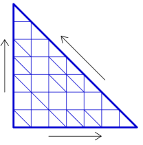
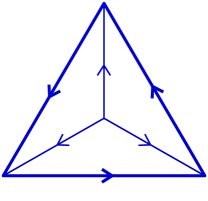
Figure 6. Assembling diagrams over $X_{T}$

Assembling three such diagrams in cyclic fashion, one obtains, for each vertex group $V$ with index triple $(i,j,k)$, a diagram of area $3\lvert{w}\rvert^{2}$ with boundary word $w(a_{i},b_{i})w(a_{j},b_{j})w(a_{k},b_{k})$. Finally, taking diagrams of the latter kind, one for each vertex of $T$, and assembling them according to $T$ (just like the triangles in $D$) one obtains a van Kampen diagram over $X_{T}$ of area $3\lvert{T}\rvert\lvert{w}\rvert^{2}$ with boundary word

$$w(a_{\nu_{0}},b_{\nu_{0}})w(a_{\nu_{1}},b_{\nu_{1}})\dotsm w(a_{\nu_{m}},b_{\nu_{m}}).$$ (7.1)

See Figure 7.

2pt $w(a_{0},b_{0})$ [t] at 18 3.5 $w(a_{9},b_{9})$ [t] at 49 3.5 $w(a_{13},b_{13})$ [tl] at 74 21 $w(a_{15},b_{15})$ [Bl] at 74.5 48 $w_{16}$ [Br] at 60.5 57 $w_{6}$ [Bl] at 35 57 $w(a_{7},b_{7})$ [Br] at 23 49 $w(a_{2},b_{2})$ [Br] at 7 23

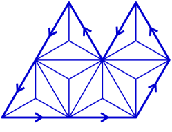
Figure 7. The canonical diagram of $w$ with boundary word (7.1), where $w_{i}=w(a_{i},b_{i})$.

In assembling this diagram, we are using the fact that $w(a_{i},b_{i})=w(a_{j},b_{j})^{-1}$ whenever $A_{i}$ and $A_{j}$ were amalgamated, which also relies on the palindromic property of $w$.

This van Kampen diagram will be called the canonical diagram of $w$, and it is defined for every palindromic word. If $w$ is reduced then the canonical diagram is also reduced.

Our remaining objective in this section is to show that canonical diagrams (and their “doubled” variants) minimize area. To this end, we need to establish some additional properties of ${\sigma}$–corridors.

Lemma 7.2.

Let $\Delta$ be a van Kampen diagram over $X_{T}$ and suppose that $C$ is a ${\sigma}$–corridor and $C^{\prime}$ is a ${\sigma}^{\prime}$–corridor in $\Delta$. If $C$ and $C^{\prime}$ have intersection of positive area, then $C\cap C^{\prime}$ contains one of the following:

1. a quadrilateral relator

2. two neighboring triangular relators with a common ${{\mathscr{S}}}_{{\sigma}}\cap{{\mathscr{S}}}_{{\sigma}^{\prime}}$–edge labeled $a_{i}$ or $b_{i}$

3. a triangular relator with a side labeled by $a_{i}$ or $b_{i}$, which is a ${{\mathscr{S}}}_{{\sigma}}\cap{{\mathscr{S}}}_{{\sigma}^{\prime}}$–edge in the boundary of $\Delta$.

We will refer to the quadrilateral relator in (1) and the union of the two neighboring triangular relators in (2) as crossing squares for $C\cap C^{\prime}$. The triangular relators in (3) will be called crossing triangles. Note that crossing squares have area $2$.

We shall see that canonical diagrams are completely filled by crossing squares and triangles for various pairs of corridors, and that these crossing regions must be present in any diagram with the same boundary.

Proof.

If case (1) does not occur, then $C\cap C^{\prime}$ contains a triangular relator. Note that ${{\mathscr{S}}}_{{\sigma}}$ has the property that a corridor cell is triangular if and only if one of its boundary ${{\mathscr{S}}}_{{\sigma}}$–edges is labeled $a_{i}$ or $b_{i}$; see Figure 5. The same is true of ${{\mathscr{S}}}_{{\sigma}^{\prime}}$. Thus, the side of the triangular relator labeled $a_{i}$ or $b_{i}$ is an ${{\mathscr{S}}}_{{\sigma}}\cap{{\mathscr{S}}}_{{\sigma}^{\prime}}$–edge. If this edge is in the boundary of $\Delta$ then case (3) occurs. Otherwise, the neighboring $2$–cell across that edge is a corridor cell for both ${{\mathscr{S}}}_{{\sigma}}$ and ${{\mathscr{S}}}_{{\sigma}^{\prime}}$ and case (2) occurs. ∎

Lemma 7.3.

If ${\sigma}$ and ${\sigma}^{\prime}$ are maximal segments in $\widehat{T}$ with no edges in common, then ${{\mathscr{S}}}_{{\sigma}}\cap{{\mathscr{S}}}_{{\sigma}^{\prime}}$ is empty and no $2$–cell is a corridor cell for both ${{\mathscr{S}}}_{{\sigma}}$ and ${{\mathscr{S}}}_{{\sigma}^{\prime}}$.

Proof.

Because $\widehat{T}$ has valence at most $3$, ${\sigma}$ and ${\sigma}^{\prime}$ must actually be disjoint. Thus, they never pass through the same triangle of $D$, which shows that ${{\mathscr{S}}}_{{\sigma}}\cap{{\mathscr{S}}}_{{\sigma}^{\prime}}$ is empty. It follows immediately that no triangular $2$–cell can be a corridor cell for both ${{\mathscr{S}}}_{{\sigma}}$ and ${{\mathscr{S}}}_{{\sigma}^{\prime}}$. The same is true for quadrilateral $2$–cells because each such $2$–cell has all of its side labels coming from a single triangle in $D$. ∎

Definition 7.4.

For each edge $e$ in $\widehat{T}$ choose maximal segments ${\sigma}_{e}$, ${\sigma}_{e}^{\prime}$ in $\widehat{T}$ whose intersection is exactly $e$. If $e$ is an interior edge, we also require that the endpoints of ${\sigma}_{e}$ and ${\sigma}_{e}^{\prime}$ are linked in the boundary of the $(\lvert{T}\rvert+2)$–gon; see Figure 8.

If $C$ and $C^{\prime}$ are ${\sigma}_{e}$– and ${\sigma}_{e}^{\prime}$–corridors respectively, a crossing square or crossing triangle for $C\cap C^{\prime}$ will be called an $e$–crossing square or an $e$–crossing triangle (or $e$–crossing region in either case). Figure 8 shows the location of $e$–crossing regions in a canonical diagram $\Delta$.

2pt * $e$ at 41.5 14 ${\color[rgb]{0.54296875,0.16796875,0.88671875}\sigma_{\!e}}$ [tl] at 49 5.5 ${\color[rgb]{0.54296875,0.16796875,0.88671875}\sigma_{\!e}}$ [Br] at 25 52 ${\color[rgb]{1,0,0}\sigma^{\prime}_{\!e}}$ [Br] at 6 20 ${\color[rgb]{1,0,0}\sigma^{\prime}_{\!e}}$ [Bl] at 72 51

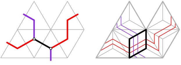
Figure 8. An edge $e$ in $\widehat{T}$ and the segments ${\sigma}_{e}$, ${\sigma}_{e}^{\prime}$. The $e$–crossing squares in $\Delta$ fill a quadrilateral region of area $2\lvert{w}\rvert^{2}$ as shown. If $e$ were a peripheral edge, the $e$–crossing squares and triangles would fill a triangular region next to the boundary of $\Delta$, of area $\lvert{w}\rvert^{2}$.

Lemma 7.5.

If $e$ and $f$ are distinct edges of $\widehat{T}$ then $e$–crossing regions and $f$–crossing regions have no $2$–cells in common.

Proof.

It suffices to show that no $2$–cell is a corridor cell simultaneously for all four corridor schemes ${{\mathscr{S}}}_{{\sigma}_{e}}$, ${{\mathscr{S}}}_{{\sigma}_{e}^{\prime}}$, ${{\mathscr{S}}}_{{\sigma}_{f}}$, ${{\mathscr{S}}}_{{\sigma}_{f}^{\prime}}$.

If $e$ and $f$ are separated by a third edge $g$, then at least one of ${\sigma}_{e}$, ${\sigma}_{e}^{\prime}$ and one of ${\sigma}_{f}$, ${\sigma}_{f}^{\prime}$ does not contain $g$. Hence, these two segments are disjoint and Lemma 7.3 applies.

Otherwise, $e$ and $f$ have a common vertex $v$. Consider the triangle in $D$ centered at $v$. There are three ways that a segment ${\sigma}$ can pass through the triangle, and the four segments must use all three of these. Of the eighteen $2$–cells associated with this triangle, one can verify easily that each $2$–cell is a corridor cell for exactly two of the three possible schemes. It follows that no $2$–cell associated with this triangle can be a corridor cell for all four corridor schemes. No other triangle in $D$ can meet all four segments, so the same is true for the other $2$–cells of $X_{T}$. ∎

Definition 7.6.

A van Kampen diagram over $X$ is called least-area if it has the smallest area of all van Kampen diagrams over $X$ having the same boundary word.

Proposition 7.7.

Let $w(x,y)$ be a reduced palindromic word. The canonical diagram of $w$ is least-area.

Proof.

Let $\Delta$ be the canonical diagram of $w$ and let $\Delta^{\prime}$ be an arbitrary van Kampen diagram with the same boundary word. Let $\ell=\lvert{w}\rvert$.

First we claim that for any choice of ${\sigma}$, say with endpoints $v_{i}$ and $v_{j}$, there are exactly $\ell$ band type ${\sigma}$–corridors in $\Delta^{\prime}$, each joining a letter in $w(a_{i},b_{i})$ with a letter in $w(a_{j},b_{j})$. Certainly, these two subwords of (7.1) contain the only occurrences of ${{\mathscr{S}}}_{{\sigma}}$–edges in the boundary of $\Delta^{\prime}$, so the number of such corridors can only be $\ell$. Also, no such corridor can join two letters of the same subword $w(a_{i},b_{i})$ or $w(a_{j},b_{j})$; using Remark 6.3 as in the proof of Proposition 6.7 one finds that $w$ must then fail to be reduced.

Now let us identify crossing squares and triangles in $\Delta^{\prime}$. If $e$ is an internal edge of $\widehat{T}$ then every ${\sigma}_{e}$–corridor crosses every ${\sigma}_{e}^{\prime}$–corridor, by the linking requirement on ${\sigma}_{e}$ and ${\sigma}_{e}^{\prime}$ (cf. Figure 8). Thus there are exactly $\ell^{2}$ $e$-crossing squares for such $e$.

If $e$ is a peripheral edge of $\widehat{T}$ incident to $v_{i}$, say, then some pairs of ${\sigma}_{e}$– and ${\sigma}_{e}^{\prime}$–corridors cross and some do not. There is one corridor of each type (${\sigma}_{e}$ or ${\sigma}_{e}^{\prime}$) emanating from each letter in the subword $w(a_{i},b_{i})$ on the boundary of $\Delta^{\prime}$, and this accounts for all ${\sigma}_{e}$– and ${\sigma}_{e}^{\prime}$–corridors. For each letter in $w(a_{i},b_{i})$ the two corridors emanating there will contain an $e$–crossing triangle; there are $\ell$ such corridor pairs. Of the remaining corridor pairs, half of them definitely cross (because their endpoints on the boundary are linked), yielding $e$–crossing squares. There are at least $\ell(\ell-1)/2$ of these. In total we have identified $e$-crossing regions of total area $2\ell^{2}$ when $e$ is an internal edge, and of total area $\ell^{2}$ when $e$ is a peripheral edge. By Lemma 7.5 we conclude that $\operatorname{Area}(\Delta^{\prime})\geqslant\operatorname{Area}(\Delta)$. ∎

Doubled canonical diagrams

For any palindromic word $w$, take the canonical diagrams of $w$ and of $w^{-1}$ and join them along their boundary subwords labeled $w(a_{\nu_{0}},b_{\nu_{0}})$ and $w(a_{\nu_{0}},b_{\nu_{0}})^{-1}$ to form a new diagram, called the doubled canonical diagram of $w$. Its boundary word is given by

$$w(a_{\nu_{1}},b_{\nu_{1}})\dotsm w(a_{\nu_{m}},b_{\nu_{m}})w(a_{\nu_{1}},b_{\nu_{1}})^{-1}\dotsm w(a_{\nu_{m}},b_{\nu_{m}})^{-1}.$$ (7.8)

If $w$ is reduced, then so is its doubled canonical diagram.

Proposition 7.9.

Let $w(x,y)$ be a reduced palindromic word. The doubled canonical diagram of $w$ is least-area.

Proof.

Let $D\Delta$ be the doubled canonical diagram of $w$ and let $\Delta^{\prime}$ be an arbitrary van Kampen diagram with the same boundary word.

Let ${\sigma}$ be a maximal segment in $\widehat{T}$ that does not contain $v_{\nu_{0}}$. The ${{\mathscr{S}}}_{{\sigma}}$–edges on the boundary of $\Delta^{\prime}$ comprise four subwords $w(a_{i},b_{i})$, $w(a_{j},b_{j})$, $w(a_{i},b_{i})^{-1}$, $w(a_{j},b_{j})^{-1}$, arranged in this cyclic ordering. We claim that the ${\sigma}$–corridors joining letters in these subwords must in fact join all the letters of $w(a_{i},b_{i})$ to those of $w(a_{j},b_{j})$, and similarly with $w(a_{i},b_{i})^{-1}$ and $w(a_{j},b_{j})^{-1}$.

First, as before, no ${\sigma}$–corridor joins two letters of the same subword, because $w$ is reduced. Next, no corridor runs between $w(a_{i},b_{i})$ and $w(a_{i},b_{i})^{-1}$ (or $w(a_{j},b_{j})$ and $w(a_{j},b_{j})^{-1}$) because then there is no room for the remaining corridors to be disjoint. Thus, the ${\sigma}$–corridors must be arranged as in Figure 9.

2pt $w_{i}$ [Bl] at 103 92 $w_{j}$ [tl] at 104 20 $w_{j}$ [Br] at 10 94 $w_{i}$ [tr] at 9 19

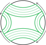
Figure 9. A configuration of $\sigma$–corridors.

It is evident that if any corridor joins $w(a_{i},b_{i})$ to $w(a_{j},b_{j})^{-1}$, then there is such a corridor joining the first letter of $w(a_{i},b_{i})$ to the last letter of $w(a_{j},b_{j})^{-1}$. If the first letter is, say, $a_{i}$ (in the orientation of the boundary of $\Delta^{\prime}$), then the corridor joins it to $a_{j}^{-1}$. On the other hand, in the canonical diagram of $w$, there is a corridor joining $a_{i}$ in the boundary to the last letter of $w(a_{j},b_{j})$, which is $a_{j}$ (because $w$ is palindromic). The existence of both corridors, even in different diagrams, contradicts the orientability of ${\mathscr{S}}_{\sigma}$ established in Remark 6.3. Therefore all corridors join $w(a_{i},b_{i})$ to $w(a_{j},b_{j})$ or $w(a_{i},b_{i})^{-1}$ to $w(a_{j},b_{j})^{-1}$, as claimed.

If ${\sigma}$ is a maximal segment with endpoints $v_{\nu_{0}}$ and $v_{i}$ then the only ${{\mathscr{S}}}_{{\sigma}}$–edges on the boundary are the two subwords $w(a_{i},b_{i})$ and $w(a_{i},b_{i})^{-1}$, and all ${\sigma}$–corridors run between them.

The rest of the proof now proceeds without difficulty just like Proposition 7.7. We have complete knowledge of which pairs of edges in the boundary of $\Delta^{\prime}$ are joined by corridors of various kinds, and these pairings are in agreement with those of $D\Delta$. One easily finds the requisite numbers of $e$–crossing regions for each $e$ and concludes that $\operatorname{Area}(\Delta^{\prime})\geqslant\operatorname{Area}(D\Delta)$. ∎

8. Snowflake diagrams

Snowflake diagrams, defined below, will be used to establish the lower bound in the proof of Theorem 10.14.

The $2$–complex $Y_{T,n}$

Recall that $S_{T,n}$ was defined via the relative presentation (3). Starting with $X_{T}$, adjoin $1$–cells and $2$–cells according to this relative presentation to obtain the $2$–complex $Y_{T,n}$ with fundamental group $S_{T,n}$. There will be $m$ new $1$–cells labeled $r_{1},\dotsc,r_{m}$ and $2m$ new $2$–cells with boundary words given by the relators of (3).

$r_{i}$–corridors

For each $i=1,\dotsc,m$ there is an orientable corridor scheme consisting of the single edge labeled $r_{i}$. It has two corridor cells which we think of as being rectangular, with sides labeled by the words

$$\varphi^{n}(a_{\nu_{i}})^{-1},\ r_{i},\ a_{\nu_{0}},\ r_{i}^{-1}$$ (8.1)

and

$$\varphi^{n}(b_{\nu_{i}})^{-1},\ r_{i},\ b_{\nu_{0}},\ r_{i}^{-1}.$$ (8.2)

The sides labeled by $a_{\nu_{0}}$ or $b_{\nu_{0}}$ will be called the short sides and the sides labeled by $\varphi^{n}(a_{\nu_{i}})^{-1}$ or $\varphi^{n}(b_{\nu_{i}})^{-1}$ the long sides of the corridor cells. The corridors for this scheme are called $r_{i}$–corridors.

Note that in any $r_{i}$–corridor in a reduced van Kampen diagram, the short sides of the corridor cells join up to form a single arc in the boundary of the corridor, labeled by a reduced word $w$ in the generators $a_{\nu_{0}}$, $b_{\nu_{0}}$. If this word happens to be monotone, then the long sides of the corridor cells also assemble to form a monotone (and reduced) word $\varphi^{n}(w)(a_{\nu_{i}},b_{\nu_{i}})$.

Snowflake diagrams

Let $w(x,y)$ be a monotone palindromic word. We will define van Kampen diagrams over $Y_{T,n}$ based on $w$ and an integer $d$ (the depth) denoted $\Delta(w,d)$. To begin, we define $\Delta(w,0)$ to be the doubled canonical diagram of $w$.

Next, to define $\Delta(w,d)$ for $d>0$, start with the diagram $\Delta(\varphi^{n}(w),d-1)$ (noting that $\varphi^{n}(w)$ is also monotone and palindromic, by our assumptions on $\varphi$). Its boundary word will have subwords of the form $\varphi^{n}(w)(a_{\nu_{i}},b_{\nu_{i}})^{\pm 1}$ for each $i=1,\dotsc,m$. Alongside each subword $\varphi^{n}(w)(a_{\nu_{i}},b_{\nu_{i}})^{\varepsilon}$ adjoin a rectangular strip made of $\lvert{w}\rvert$ $2$–cells whose four sides are labeled by the words

$$\varphi^{n}(w)(a_{\nu_{i}},b_{\nu_{i}})^{-\varepsilon},\ r_{i},\ w(a_{\nu_{0}},b_{\nu_{0}})^{\varepsilon},\ r_{i}^{-1}.$$

Then, adjoin a copy of the canonical diagram of $w^{-\varepsilon}$, which contains a side labeled $w(a_{\nu_{0}},b_{\nu_{0}})^{-\varepsilon}$.

Doing this for each subword as described, one obtains $\Delta(w,d)$. See Figure 10. Note that the boundary of $\Delta(w,d)$ contains many copies of the subwords $w(a_{\nu_{i}},b_{\nu_{i}})^{\pm 1}$ for each $i=1,\dotsc,m$. In fact, it is easy to verify by induction on $d$ that the boundary word is made entirely of copies of these words, together with occurrences of the letters $r_{i}^{\pm 1}$.

2pt ${\color[rgb]{0,0,0.81640625}\vdots}$ [B] at 146.5 113 ${\color[rgb]{0,0,0.81640625}\vdots}$ [t] at 216.5 50.5 * ${\color[rgb]{0,0,0.81640625}\vdots}$ at 98.5 138 * ${\color[rgb]{0,0,0.81640625}\vdots}$ at 26 142.5 * ${\color[rgb]{0,0,0.81640625}\vdots}$ at 178 22 * ${\color[rgb]{0,0,0.81640625}\vdots}$ at 1 68 * ${\color[rgb]{0,0,0.81640625}\vdots}$ at 2 10

$w_{0}$ [tl] at 251 75 $w_{1}$ [tr] at 261 49 $w_{2}$ [tl] at 284 49.5 $w_{3}$ [Bl] at 293.5 75 $w_{4}$ [B] at 271 95.5

$w_{0}$ [Bl] at 237 120 $w_{1}$ [tl] at 262.5 114.5 $w_{2}$ [Bl] at 272.5 140 $w_{3}$ [B] at 250 161 $w_{4}$ [Br] at 230 148

$w_{0}$ [Br] at 196 121 $w_{1}$ [Bl] at 200.5 148 $w_{2}$ [B] at 182 161 $w_{3}$ [Br] at 158.5 141 $w_{4}$ [tr] at 165 118

$\varphi^{n}w_{2}$ [Br] at 242 77 $\varphi^{n}w_{0}$ [Bl] at 187.5 82 $\varphi^{2n}w_{3}$ [tr] at 178.5 81 $\varphi^{2n}w_{0}$ [tl] at 112 74 $\varphi^{3n}w_{1}$ [Br] at 102 76.6 $\varphi^{3n}w_{0}$ [B] at 63 52 $\varphi^{4n}w_{3}$ [t] at 63 37

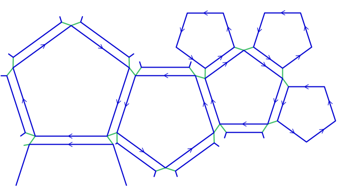
Figure 10. Part of the snowflake diagram $\Delta(w,d)$, with $m=4$ (and $d\geqslant 4$). The word $\varphi^{in}(w)(a_{\nu_{j}},b_{\nu_{j}})$ is abbreviated as $\varphi^{in}w_{j}$. The pentagonal regions are canonical diagrams and the strips between them are $r_{j}$–corridors for various $j$.

Note that $\Delta(w,d)$ contains a sub-diagram $\Delta(\varphi^{in}(w),d-i)$ for each $i$ between $0$ and $d$. In particular, it contains a copy of $\Delta(\varphi^{dn}(w),0)$, which is a doubled canonical diagram of area $6\lvert{T}\rvert\lvert{\varphi^{dn}(w)}\rvert^{2}$.

Proposition 8.3.

Let $w(x,y)$ be a monotone palindromic word. For each $d\geqslant 0$ the diagram $\Delta(w,d)$ is least-area.

Proof.

First note that $\Delta(w,d)$ is reduced, since it is made of reduced sub-diagrams, separated by reduced $r_{i}$–corridors, which have no $2$–cells in common with the sub-diagrams. (The sub-diagrams being reduced depends on the monotonicity of $w$, which implies that the words $\varphi^{in}(w)$ are reduced.)

Now suppose that $d=0$ and let $\Delta^{\prime}$ be any reduced diagram over $Y_{T,n}$ with the same boundary as $\Delta(w,0)$. We claim that there are no $r_{i}$–corridors for any $i$. If there were, they would be of annulus type, and the short side of the corridor would be labeled by a cyclically reduced word $v(a_{\nu_{0}},b_{\nu_{0}})$ representing the trivial element. Since $A_{\nu_{0}}$ is free on $a_{\nu_{0}},b_{\nu_{0}}$, no such corridors can exist. Therefore $\Delta^{\prime}$ is actually a diagram over $X_{T}$, and Proposition 7.9 says that $\operatorname{Area}(\Delta^{\prime})\geqslant\operatorname{Area}(\Delta(w,0))$.

Proceeding by induction on $d$, suppose that $d\geqslant 1$ and $\Delta^{\prime}$ is a reduced diagram over $Y_{T,n}$ of smallest area, with the same boundary as $\Delta(w,d)$. As before, there can be no $r_{i}$–corridors of annulus type. There will be band type $r_{i}$–corridors joining occurrences of $r_{i}^{\pm 1}$ on the boundary. Note that $r_{i}$– and $r_{j}$–corridors cannot cross for any $i,j$ (no $2$–cell is a corridor cell for both corridor schemes). Hence the $r_{i}$–edges on the boundary must be paired by corridors in the same way as in $\Delta(w,d)$.

Consider an outermost $r_{i}$–corridor. Its complement in $\Delta^{\prime}$ is two sub-diagrams, one of which is a diagram over $X_{T}$ with boundary word

$$\widehat{w}(a_{\nu_{0}},b_{\nu_{0}})^{\varepsilon}w(a_{\nu_{1}},b_{\nu_{1}})^{\varepsilon}\dotsm w(a_{\nu_{m}},b_{\nu_{m}})^{\varepsilon}$$

for some word $\widehat{w}$ and some $\varepsilon=\pm 1$. Here, $\widehat{w}(a_{\nu_{0}},b_{\nu_{0}})$ is the word along the short side of the corridor. Recall that in $V_{T}$, the word $w(a_{\nu_{1}},b_{\nu_{1}})^{\varepsilon}\dotsm w(a_{\nu_{m}},b_{\nu_{m}})^{\varepsilon}$ represents the element $w(a_{\nu_{0}},b_{\nu_{0}})^{-\varepsilon}$, which moreover is in the free subgroup $A_{\nu_{0}}$. Since $\widehat{w}(a_{\nu_{0}},b_{\nu_{0}})$ is reduced, it must equal $w(a_{\nu_{0}},b_{\nu_{0}})$. It follows that the corridor, considered as a sub-diagram, is identical to the corresponding corridor in $\Delta(w,d)$. Also, the part of $\Delta^{\prime}$ on the short side of the corridor is a diagram over $X_{T}$ with the same boundary as the canonical diagram of $w^{\varepsilon}$. By Proposition 7.7 its area agrees with that of the canonical diagram.

Taking all the outermost $r$–corridors and the sub-diagrams that they separate from the central region in $\Delta^{\prime}$, we have found that these have total area equal to the corresponding regions in $\Delta(w,d)$. Moreover, if we delete these regions, the resulting boundary word is the boundary word of the corresponding sub-diagram $\Delta(\varphi^{n}(w),d-1)$ of $\Delta(w,d)$. By induction, the central portion of $\Delta^{\prime}$ has area equal to that of $\Delta(\varphi^{n}(w),d-1)$ and we are done. ∎

9. Folded corridors and subgroup distortion

The main result of this section is Proposition 9.7 (and its variant Corollary 9.14) which bounds the distortion of the edge group $A_{\nu_{0}}$ in $S_{T,n}$. After discussing some preliminaries, we proceed to study folded corridors, culminating in Lemma 9.5. This lemma plays an important role in the proof of Proposition 9.7, which occupies the rest of the section.

Define the standard generating set for $S_{T,n}$ to be the standard generating set for $V_{T}$ together with the generators $r_{1},\dotsc,r_{m}$. Recall that the former generators include all generators $x_{i}$ and $y_{i}$, and the peripheral generators $a_{\nu_{i}}$, $b_{\nu_{i}}$ ($i=0,\dotsc,m$).

For $g\in A_{\nu_{i}}$ let $\lvert{g}\rvert_{A_{\nu_{i}}}$ denote the length of the reduced word in the basis $a_{\nu_{i}}$, $b_{\nu_{i}}$ representing $g$. Similarly, let $\lVert{g}\rVert_{A_{\nu_{i}}}$ be the weighted word length of the reduced representative (cf. Definition 6.5). Recall that the letters $a_{i}^{\pm 1}$ and $x_{i}^{\pm 1}$ have weight $1+\sqrt{2}$ and the letters $b_{i}^{\pm 1}$ and $y_{i}^{\pm 1}$ have weight $1$. Let the letters $r_{i}^{\pm 1}$ also be given weight $1$.

Now we assign lengths to the edges of $Y_{T,n}$, and correspondingly to the edges in any van Kampen diagram over $Y_{T,n}$, as follows. Edges labeled by $x_{i}$ or $a_{i}$ are given length $1+\sqrt{2}$, and all other edges (those labeled $y_{i}$, $b_{i}$, or $r_{i}$) are given length $1$. In this section, lengths of paths in a van Kampen diagram will always be meant with respect to these edge lengths.

With this convention, the length of a path in the $1$–skeleton will agree with the weighted length of the word labeling it.

Folded corridors

Recall that each $r_{i}$–corridor cell has a short side and a long side. In any $r_{i}$–corridor, the embedded open annulus or open band inside it separates all of the short sides of the corridor cells from the long sides.

The boundary of an $r_{i}$–corridor is a $1$–complex containing zero or two $r_{i}$–edges. The partial boundary is defined to be the boundary with the interiors of the $r_{i}$–edges removed.

If $C$ is an $r_{i}$–corridor in a reduced diagram, then the short sides of its cells join to form a component of the partial boundary which is labeled by a reduced word in the generators $a_{\nu_{0}}$, $b_{\nu_{0}}$. If $C$ were of annulus type, then we would have a cyclically reduced word in the free group $A_{\nu_{0}}$ representing the trivial element. Hence, $C$ must be of band type.

Following [BG10], a band type $r_{i}$–corridor is called folded if it is reduced and every component of its partial boundary is labeled by a reduced word in the generators of $S_{T,n}$. We have noted already that the short sides of corridor cells form a single such component, which we now call the bottom of the corridor. Any other component is labeled by a reduced word in the generators $a_{\nu_{i}}$, $b_{\nu_{i}}$. Again, such a component cannot be a loop (since $A_{\nu_{i}}$ is free) and hence there is only one other component, which we call the top of the corridor. If $w(a_{\nu_{0}},b_{\nu_{0}})$ is the reduced word along the bottom, then the top is labeled by the reduced word in $a_{\nu_{i}}$, $b_{\nu_{i}}$ representing $\varphi^{n}(w)(a_{\nu_{i}},b_{\nu_{i}})$.

Remark 9.1.

Given any reduced word $w(a_{\nu_{0}},b_{\nu_{0}})$, one can build a folded corridor with bottom labeled by $w$. Start by joining corridor cells end to end along $r_{i}$–edges to form a corridor with bottom side labeled by $w$. Then, the long sides of the corridor cells form an arc labeled by a possibly unreduced word representing $\varphi^{n}(w)(a_{\nu_{i}},b_{\nu_{i}})$. By successively folding together adjacent pairs of edges along the top (with matching labels), one eventually obtains a folded corridor. Each folding operation corresponds to a free reduction in the word labeling the top side of the corridor. The final word along the top of the folded corridor is uniquely determined (being the reduced form of $\varphi^{n}(w)(a_{\nu_{i}},b_{\nu_{i}})$) but the internal structure will depend on the particular sequence of folds chosen.

Let $C$ be a folded $r_{i}$–corridor. Define $S\subset C$ to be the smallest subcomplex containing all the $r_{i}$–edges, and all the open $1$–cells which lie in the interior of $C$ (informally, the seams in $C$). Note that $S$ contains exactly those edges of $C$ that are not in the top or bottom.

Lemma 9.2.

Let $S_{0}$ be a connected component of $S$. Then

1. $S_{0}$ is a tree;

2. $S_{0}$ contains exactly one vertex in the top of $C$;

3. every valence-one vertex in $S_{0}$ lies in the top or bottom of $C$.

Conclusions (2) and (3) imply that $S_{0}$ contains at least one vertex in the bottom of $C$.

Proof.

First note that every $2$–cell of $C$ meets the bottom in exactly one edge. Conclusion (1) follows immediately since a loop in $S_{0}$ would separate a $2$–cell from the bottom. For the same reason, $S_{0}$ cannot contain two or more vertices of the top.

A second observation is that the boundary of every $2$–cell is labeled by a cyclically reduced word (namely, (8.1) or (8.2)). Hence no two adjacent edges of the same cell can be folded together. Therefore $S_{0}$ cannot have a valence-one vertex in the interior of $C$, whence (3).

It remains to show that $S_{0}$ contains a vertex of the top. If not, then it is separated from the top by a $2$–cell which then must meet the bottom in a disconnected set, contradicting the initial observation above. ∎

Let $p$ be a vertex in the top of $C$ and $q$ a vertex in the bottom. We say that $p$ is above $q$ if both vertices are in the same connected component of $S$. We have the following “bounded cancellation” lemma, which is a restatement of Lemma 1.2.4 of [BG10]:

Lemma 9.3.

There is a constant $K_{0}=K_{0}(\varphi^{n})$ such that if $p$ is a vertex in the top of a folded corridor and $q_{1}$, $q_{2}$ are vertices that are both below $p$, then the sub-segment $[q_{1},q_{2}]$ of the bottom has at most $K_{0}$ edges. ∎

For vertices $p$ in the top and $q$ in the bottom, we say that $p$ is nearly above $q$ if there is a vertex $p^{\prime}$ above $q$ such that $p$ and $p^{\prime}$ are in the boundary of a common $2$–cell. It is clear that every vertex in the top is nearly above some vertex on the bottom.

Lemma 9.4.

There is a constant $K_{1}=K_{1}(\varphi^{n})$ such that if $C$ is a folded corridor and $p$ is nearly above $q$ in $C$, then there is a path in the $1$–skeleton of $C$ from $p$ to $q$, containing no bottom edges, of length at most $K_{1}$.

Proof.

Let $L$ be the maximum of the boundary lengths of the two $r_{i}$–corridor cells. Let $p^{\prime}$ be a vertex above $q$ such that $p$ and $p^{\prime}$ are in the boundary of a common $2$–cell $e^{2}$, and let $S_{0}$ be the component of $S$ containing $p^{\prime}$ and $q$. Let $q^{\prime}$ be the unique bottom vertex of $S_{0}$ which is in the boundary of $e^{2}$. There are paths $[p,p^{\prime}]$ in the top and $[p^{\prime},q^{\prime}]$ in $S_{0}$. These have total length at most $L$, since they are in the boundary of $e^{2}$.

Next, any two adjacent bottom vertices in $S_{0}$ are in the boundary of a $2$–cell, and hence are joined by a path in $S_{0}$ of length at most $L$. It follows that $q^{\prime}$ and $q$ are joined by a path $[q^{\prime},q]$ in $S_{0}$ of length at most $K_{0}L$, with $K_{0}$ given by Lemma 9.3. Now the path $[p,p^{\prime}]\cdot[p^{\prime},q^{\prime}]\cdot[q^{\prime},q]$ has length at most $K_{1}=(K_{0}+1)L$. ∎

Lemma 9.5.

There is a constant $K_{2}=K_{2}(\varphi^{n})$ such that if $C$ is a folded corridor and $[p_{1},p_{2}]$, $[q_{1},q_{2}]$ are sub-segments of the top and bottom, respectively, with $p_{j}$ nearly above $q_{j}$ for $j=1,2$, and $u(a_{\nu_{i}},b_{\nu_{i}})$ is the word labeling $[p_{1},p_{2}]$, then

$$\lVert{\varphi^{-n}(u)}\rVert_{A_{\nu_{i}}}-\ K_{2}\ \leqslant\ \lvert{[q_{1},q_{2}]}\rvert\ \leqslant\ \lVert{\varphi^{-n}(u)}\rVert_{A_{\nu_{i}}}+\ K_{2}.$$

The essential point is that the length of $[q_{1},q_{2}]$ is determined, up to an additive error, by the word $u$ labeling $[p_{1},p_{2}]$. (It is certainly not determined by the length of $[p_{1},p_{2}]$ alone.)

Proof.

Let $w(a_{\nu_{0}},b_{\nu_{0}})$ be the reduced word labeling $[q_{1},q_{2}]$. Let $\widehat{S}$ be the union of $S$ and the top of $C$. For $j=1,2$ let $[q_{j},p_{j}]$ be a shortest path in $\widehat{S}$ from $q_{j}$ to $p_{j}$. Its first edge is an $r_{i}$–edge labeled $r_{i}^{-1}$, and so the label on $[q_{j},p_{j}]$ has the form $r_{i}^{-1}\cdot v_{j}(a_{\nu_{i}},b_{\nu_{i}})$ for some reduced word $v_{j}$. This word has weighted length less than $K_{1}$ by Lemma 9.4.

The four segments form a relation in $S_{T,n}$, namely

$$w(a_{\nu_{0}},b_{\nu_{0}})\ =\ r_{i}^{-1}v_{1}(a_{\nu_{i}},b_{\nu_{i}})u(a_{\nu_{i}},b_{\nu_{i}})v_{2}(a_{\nu_{i}},b_{\nu_{i}})^{-1}r_{i}$$

$$=\ \varphi^{-n}(v_{1})(a_{\nu_{0}},b_{\nu_{0}})\,\varphi^{-n}(u)(a_{\nu_{0}},b_{\nu_{0}})\,\varphi^{-n}(v_{2})(a_{\nu_{0}},b_{\nu_{0}}).$$ (9.6)

This is an equality of elements of the free subgroup $A_{\nu_{0}}$. Now define

$$K_{2}\ =\ 2\max\left\{\lVert{\varphi^{-n}(v)}\rVert_{A_{\nu_{0}}}\mid v\text{ is a word in }a_{\nu_{0}},b_{\nu_{0}}\text{ of weighted length }<K_{1}\right\}.$$

Observe that the left hand side of (9.6) has reduced weighted length $\lvert{[q_{1},q_{2}]}\rvert$ and the right hand side has reduced weighted length within $K_{2}$ of $\lVert{\varphi^{-n}(u)(a_{\nu_{0}},b_{\nu_{0}})}\rVert_{A_{\nu_{0}}}$, which is equal to $\lVert{\varphi^{-n}(u)}\rVert_{A_{\nu_{i}}}$. ∎

We turn now to the main result of this section, the bound on edge group distortion. Recall from the Introduction that the proof is an inductive proof based on Britton’s Lemma. It falls into two cases, requiring very different methods.

In the first case, the proof is based on a method from [BB00]. It is the balancing property of $V_{T}$ that allows us to carry out this argument. The crucial moment occurs in (9.8) and the choice of index $j^{\prime}$, and the subsequent reasoning.

The second case makes use of folded corridors and Lemma 9.5. The overvall induction argument is based on the nested structure of $r_{j}$–corridors in a van Kampen diagram. If these corridors are always oriented in the correct direction, then the argument based on the balancing property would suffice. If there exists a backwards-facing $r_{j}$–corridor, then the inductive process will inevitably land in Case II.

The backwards-facing corridor may then introduce geometric effects that adversely affect the inductive calculation. When this occurs, we prove that there will be correctly oriented corridors just behind the first one, and perfectly matching segments along these corridors, along which any metric distortion introduced by the first corridor is exactly undone. This occurs in (9.9), using Lemma 9.5. This argument also depends crucially on $\sigma$–corridors.

Proposition 9.7 (Edge group distortion).

Given $T$ and $n$ there is a constant $K_{3}$ such that if $w$ is a word in the standard generators of $S_{T,n}$ representing an element $g\in A_{\nu_{0}}$ then

$$\lVert{g}\rVert_{A_{\nu_{0}}}\ \leqslant\ K_{3}\lVert{w}\rVert^{\alpha}$$

where $\alpha=n\log_{m}(\lambda)$.

Proof.

Let $K_{3}\ =\ \max\{1,3K_{2}/2,\Lambda^{\!n}\}$ where $K_{2}$ is given by Lemma 9.5 and $\Lambda$ is the maximum stretch factor for $\varphi^{-1}$ with respect to the weighted word length $\lVert{\,\cdot\,}\rVert$.

The universal cover $\widetilde{Y}_{T,n}$ is the total space of a tree of spaces, with vertex spaces equal to copies of the universal cover $\widetilde{X}_{T}$. Every $1$–cell of $\widetilde{Y}_{T,n}$ is either contained in a vertex space, or is labeled $r_{j}^{\pm 1}$ for some $j$ and has endpoints in two neighboring vertex spaces.

We argue by induction on the number of occurrences of $r_{j}^{\pm 1}$ in $w$ (for all $j$). We may assume that $w$ is a shortest word in the generators of $S_{T,n}$ representing $g$. This word describes a labeled geodesic in the $1$–skeleton of $\widetilde{Y}_{T,n}$ with endpoints in the same vertex space. Using the tree structure, one finds a decomposition of $w$ as $w_{1}\dotsm w_{k}$ where each $w_{i}$ satisfies one of the following:

1. $w_{i}=r_{j}u_{i}r_{j}^{-1}$ for some $j$ and $w_{i}$ represents an element of $A_{\nu_{j}}$. Let $v_{i}(a_{\nu_{j}},b_{\nu_{j}})$ be the reduced word representing $w_{i}$ in this case.

2. $w_{i}=r_{j}^{-1}u_{i}r_{j}$ for some $j$ and $w_{i}$ represents an element of $A_{\nu_{0}}$. Let $v_{i}(a_{\nu_{0}},b_{\nu_{0}})$ be the reduced word representing $w_{i}$ in this case.

3. $w_{i}$ is a word in the generators $a_{\nu_{j}}$, $b_{\nu_{j}}$ for some $j$.

4. $w_{i}$ is a word in the generators $\{x_{j},y_{j}\}$ (allowing all $j$).

Let $v_{i}=w_{i}$ in cases (3) and (4), and define $v=v_{1}\dotsm v_{k}$. The proof now splits into cases, based on the structure of the decomposition $w=w_{1}\dotsm w_{k}$.

• Case IA:  all subwords $w_{i}$ are of types (3) or (4). This is simply the base case of the induction.

• Case IB:  either there is a subword $w_{i}$ of type (1), or there are two or more subwords of type (2).

• Case II:  exactly one subword $w_{i}$ is of type (2) and all others are of types (3) or (4).

Proof in Cases IA and IB.  Define the sets

$$I_{j}\ =\ \{\,i\mid v_{i}\text{ is a word in the generators }a_{\nu_{j}},b_{\nu_{j}}\,\},$$

$$I_{xy}\ =\ \{\,i\mid v_{i}\text{ is a word in the generators }\{x_{j},y_{j}\}\,\}.$$

Note that $\lVert{v}\rVert_{\nu_{j}}=\sum_{i\in I_{j}}\lVert{v_{i}}\rVert$ and $\lVert{v}\rVert_{x}+\lVert{v}\rVert_{y}=\sum_{i\in I_{xy}}\lVert{v_{i}}\rVert$. We begin by establishing two claims.

Claim 1: if $i\in I_{j}$ and $j\not=0$ then $\lVert{v_{i}}\rVert\leqslant K_{3}(m\lVert{w_{i}}\rVert)^{\alpha}$. If $w_{i}$ satisfies (3) then the claim is trivial: $\lVert{v_{i}}\rVert=\lVert{w_{i}}\rVert\leqslant K_{3}(m\lVert{w_{i}}\rVert)^{\alpha}$ since $K_{3},m,\alpha\geqslant 1$. Otherwise, $w_{i}$ satisfies (1) and $w_{i}=r_{j}u_{i}r_{j}^{-1}$ where $u_{i}$ represents an element of $A_{\nu_{0}}$. Let $z_{i}$ be the reduced word in $a_{\nu_{0}}$, $b_{\nu_{0}}$ equal to $u_{i}$ in $A_{\nu_{0}}$, and note that $\varphi^{n}(z_{i})(a_{\nu_{j}},b_{\nu_{j}})=v_{i}$ in $A_{\nu_{j}}$. Since $v_{i}$ is reduced we have

$$\lVert{v_{i}}\rVert\ \leqslant\ \lVert{\varphi^{n}(z_{i})(a_{\nu_{j}},b_{\nu_{j}})}\rVert\ =\ \lVert{\varphi^{n}(z_{i})}\rVert\ \leqslant\ \lambda^{n}\lVert{z_{i}}\rVert\ =\ \lambda^{n}\lVert{u_{i}}\rVert_{A_{\nu_{0}}}\ =\ m^{\alpha}\lVert{u_{i}}\rVert_{A_{\nu_{0}}}.$$

Here, the second inequality follows from Lemma 6.6. The final quantity is at most

$$K_{3}m^{\alpha}(\lVert{w_{i}}\rVert-2)^{\alpha}\leqslant K_{3}(m\lVert{w_{i}}\rVert)^{\alpha}$$

by the induction hypothesis.

Claim 2: if $i\in I_{0}\cup I_{xy}$ then $\lVert{v_{i}}\rVert\leqslant K_{3}\lVert{w_{i}}\rVert^{\alpha}$. As in Claim 1, if $w_{i}$ satisfies (3) or (4) then Claim 2 is trivially true. The remaining case is when $w_{i}$ satisfies (2). Now the claim is an instance of the induction hypothesis: since $v_{i}$ is reduced we have $\lVert{v_{i}}\rVert=\lVert{w_{i}}\rVert_{A_{\nu_{0}}}\leqslant K_{3}\lVert{w_{i}}\rVert^{\alpha}$. Note that the induction hypothesis applies precisely because we are not in Case II, and $w_{i}$ contains fewer occurrences of the letters $r_{j}^{\pm 1}$ than $w$.

Among the indices $1,\dotsc,m$, choose $j^{\prime}$ to minimize the sum $\sum_{i\in I_{j^{\prime}}}\lVert{w_{i}}\rVert$. Thus we have

$$m\sum_{i\in I_{j^{\prime}}}\lVert{w_{i}}\rVert\ \leqslant\ \sum_{i\in I_{1}\cup\dotsb\cup I_{m}}\lVert{w_{i}}\rVert.$$ (9.8)

Observe that $v=v_{1}\dotsm v_{k}$ is a word in the standard generators of $V_{T}$ representing the element $g$. Applying Proposition 6.7 (and Remark 6.9) to this word yields the inequality

$$\lVert{g}\rVert_{A_{\nu_{0}}} \leqslant\ \lVert{v}\rVert_{\nu_{0}}+\lVert{v}\rVert_{x}+\lVert{v}\rVert_{y}+\lVert{v}\rVert_{\nu_{j^{\prime}}}$$

$$=\ \sum_{i\in I_{0}}\lVert{v_{i}}\rVert\ +\sum_{i\in I_{xy}}\lVert{v_{i}}\rVert\ +\sum_{i\in I_{j^{\prime}}}\lVert{v_{i}}\rVert.$$

Then we have

$$\lVert{g}\rVert_{A_{\nu_{0}}}\ \leqslant\sum_{i\in I_{0}\cup I_{xy}}K_{3}\lVert{w_{i}}\rVert^{\alpha}\ +\sum_{i\in I_{j^{\prime}}}K_{3}\left(m\lVert{w_{i}}\rVert\right)^{\alpha}$$

$$\leqslant\sum_{i\in I_{0}\cup I_{xy}}K_{3}\lVert{w_{i}}\rVert^{\alpha}\ +\ K_{3}\left(\sum_{i\in I_{j^{\prime}}}m\lVert{w_{i}}\rVert\right)^{\alpha}$$

by Claims 1 and 2, and

$$\lVert{g}\rVert_{A_{\nu_{0}}}\ \leqslant\sum_{i\in I_{0}\cup I_{xy}}K_{3}\lVert{w_{i}}\rVert^{\alpha}\ +\ K_{3}\left(\sum_{i\in(I_{1}\cup\dotsb\cup I_{m})}\lVert{w_{i}}\rVert\right)^{\alpha}$$

$$\leqslant\ K_{3}\left(\sum_{i}\lVert{w_{i}}\rVert\right)^{\alpha}$$

$$=\ K_{3}\lVert{w}\rVert^{\alpha}$$

By (9.8).

Proof in Case II.  In this case we write $w$ as $w_{L}\hat{w}w_{R}$ where $\hat{w}$ is the subword of type (2) and $w_{L}$, $w_{R}$ are products of subwords of types (3) and (4). Thus $\hat{w}=r^{-1}_{{j^{\prime}}}ur_{{j^{\prime}}}$ for some index ${j^{\prime}}\not=0$, where $u$ represents an element of $A_{\nu_{{j^{\prime}}}}$. Let $\hat{v}$ be the reduced word in $a_{\nu_{0}},b_{\nu_{0}}$ representing $\hat{w}$, and let $\hat{u}$ be the reduced word in $a_{\nu_{{j^{\prime}}}},b_{\nu_{{j^{\prime}}}}$ representing $u$.

We proceed by decomposing the word $u$ using the tree of spaces structure of $\widetilde{Y}_{T,n}$. First, choose an index ${j^{\prime\prime}}\not={j^{\prime}}$ from the set $\{1,\dotsc,m\}$. Then write $u=\hat{w}_{1}\dotsm\hat{w}_{k^{\prime}}$ where each $\hat{w}_{i}$ satisfies one of the following:

1. $\hat{w}_{i}=r_{{j^{\prime}}}\hat{u}_{i}r_{{j^{\prime}}}^{-1}$ or $\hat{w}_{i}=r_{{j^{\prime\prime}}}\hat{u}_{i}r_{{j^{\prime\prime}}}^{-1}$. Let $\hat{v}_{i}$ be the reduced word in $a_{\nu_{j^{\prime}}},b_{\nu_{j^{\prime}}}$ or $a_{\nu_{j^{\prime\prime}}},b_{\nu_{j^{\prime\prime}}}$ representing $\hat{w}_{i}$.

2. $\hat{w}_{i}=r_{j}\hat{u}_{i}r_{j}^{-1}$ for some $j\not={j^{\prime}},{j^{\prime\prime}}$. Let $\hat{v}_{i}(a_{\nu_{j}},b_{\nu_{j}})$ be the reduced word representing $\hat{w}_{i}$.

3. $\hat{w}_{i}=r_{j}^{-1}\hat{u}_{i}r_{j}$ for some $j$. Let $\hat{v}_{i}(a_{\nu_{0}},b_{\nu_{0}})$ be the reduced word representing $\hat{w}_{i}$.

4. $\hat{w}_{i}$ is a word in the standard generators of $V_{T}$. Let $\hat{v}_{i}=\hat{w}_{i}$ in this case.

There is an equality $\hat{u}=\hat{v}_{1}\dotsm\hat{v}_{k^{\prime}}$ in $V_{T}$. Let $\Delta$ be a van Kampen diagram over $X_{T}$ with boundary word $\hat{v}_{1}\dotsm\hat{v}_{k^{\prime}}\hat{u}^{-1}$. The arcs in the boundary of $\Delta$ labeled by the words $\hat{v}_{i}$ or $\hat{u}^{-1}$ are called the sides of $\Delta$. The side labeled by $\hat{v}_{i}$ is declared to be of type (5), (6), (7), or (8) accordingly as $\hat{w}_{i}$ is of one of these types. The remaining side will be regarded as being oriented in the opposite direction, so that its label reads $\hat{u}$.

We enlarge $\Delta$ to a diagram $\Delta^{\prime}$ by adjoining folded $r$–corridors, as follows. First, for each subword $\hat{w}_{i}$ of type (5), build a folded corridor $C_{i}$ whose top is labeled by $\hat{v}_{i}$ and whose bottom is labeled by the reduced word in $a_{\nu_{0}},b_{\nu_{0}}$ representing $\hat{u}_{i}$ in $A_{\nu_{0}}$. Adjoin this corridor to $\Delta$ along the side labeled by $\hat{v}_{i}$. Next, build a folded $r_{j^{\prime}}$–corridor $C_{0}$ whose top is labeled by $\hat{u}$ and whose bottom is labeled by $\hat{v}$. Adjoin it to $\Delta$ along the side labeled by $\hat{u}$. The resulting diagram is $\Delta^{\prime}$.

Now let $\sigma\subset\widehat{T}$ be the maximal segment whose endpoints correspond to the peripheral subgroups $A_{\nu_{j^{\prime}}}$ and $A_{\nu_{j^{\prime\prime}}}$. The corridor scheme ${\mathscr{S}}_{\sigma}$ defines $\sigma$–corridors in $\Delta$. Every edge in the side labeled $\hat{u}$ has a $\sigma$–corridor emanating from it, landing on a side of type (5) or (8). (They cannot land on the other sides, because their edges are not members of ${\mathscr{S}}_{\sigma}$. They cannot land on the side labeled $\hat{u}$, because $\hat{u}$ is reduced; cf. the proof of Proposition 6.7.) Decompose $\hat{u}$ as $z_{1}\dotsm z_{\ell}$ such that

• for each $z_{i}$, the $\sigma$–corridors emanating from the edges labeled by $z_{i}$ either land on a single side of type (5), or on a union of sides of type (8)

• each $z_{i}$ is maximal with respect to the preceding property.

Let $p_{0},\dotsc,p_{\ell}$ be the vertices along the side labeled $\hat{u}$ such that for each $i$, the arc labeled by $z_{i}$ has endpoints $p_{i-1}$ and $p_{i}$. These vertices lie along the top of the folded $r_{j^{\prime}}$–corridor $C_{0}$. Choose vertices $q_{0},\dotsc,q_{\ell}$ along the bottom of $C_{0}$ such that $p_{i}$ is nearly above $q_{i}$ for each $i$ and $q_{0},q_{\ell}$ are the endpoints of the bottom. Let $[p_{i-1},p_{i}]$ and $[q_{i-1},q_{i}]$ denote the segments along the top and bottom, respectively, with the indicated endpoints.

Next define the index sets

$$I_{\textup{\maketag@@@{(\ignorespaces{\ref{hw1}}\@@italiccorr)}}}\ =\ \{i\mid\text{ the $\sigma$--corridors emanating from $z_{i}$ land on a side of type {\maketag@@@{(\ignorespaces{\ref{hw1}}\@@italiccorr)}}}\},$$

$$I_{\textup{\maketag@@@{(\ignorespaces{\ref{hw4}}\@@italiccorr)}}}\ =\ \{i\mid\text{ the $\sigma$--corridors emanating from $z_{i}$ land on sides of type {\maketag@@@{(\ignorespaces{\ref{hw4}}\@@italiccorr)}}}\}$$

so that $I_{\textup{\maketag@@@{(\ignorespaces{\ref{hw1}}\@@italiccorr)}}}\cup I_{\textup{\maketag@@@{(\ignorespaces{\ref{hw4}}\@@italiccorr)}}}=\{1,\dotsc,\ell\}$. For each $i\in I_{\textup{\maketag@@@{(\ignorespaces{\ref{hw1}}\@@italiccorr)}}}$ let $j_{i}$ be the index such that the $\sigma$–corridors emanating from $z_{i}$ land on the side labeled by $\hat{v}_{j_{i}}$.

If $C$ and $C^{\prime}$ are two $\sigma$–corridors emanating from $\hat{u}$ and landing on the same side $\hat{v}_{j}$, then every corridor emanating from $\hat{u}$ between $C$ and $C^{\prime}$ must also land on $\hat{v}_{j}$, since corridors do not cross. Moreover, if $C$ and $C^{\prime}$ are adjacent in $\hat{u}$ then they will land on adjacent edges of $\hat{v}_{j}$; otherwise, any $\sigma$–corridor emanating from $\hat{v}_{j}$ between $C$ and $C^{\prime}$ is forced to land on $\hat{v}_{j}$, contradicting that $\hat{v}_{j}$ is reduced.

These remarks imply that for every $i\in I_{\textup{\maketag@@@{(\ignorespaces{\ref{hw1}}\@@italiccorr)}}}$, the corridors emanating from $z_{i}$ land on a connected subarc $\alpha_{i}$ of the side labeled $\hat{v}_{j_{i}}$, and in fact the label along $\alpha_{i}$ is the word $z_{i}(a_{\nu_{j^{\prime}}},b_{\nu_{j^{\prime}}})$ or $z_{i}(a_{\nu_{j^{\prime\prime}}},b_{\nu_{j^{\prime\prime}}})$, by Remark 6.3. Note that $\alpha_{i}$ lies along the top of the $r$–corridor $C_{j_{i}}$. Let $\beta_{i}$ be a subarc of the bottom of $C_{j_{i}}$ such that the endpoints of $\alpha_{i}$ are nearly above those of $\beta_{i}$. Since $[p_{i-1},p_{i}]$ and $\alpha_{i}$ are labeled by the same word, we have

$$\lvert{\lvert{[q_{i-1},q_{i}]}\rvert-\lvert{\beta_{i}}\rvert}\rvert\ \leqslant\ 2K_{2}$$ (9.9)

by Lemma 9.5. Therefore,

$$\lvert{[q_{i-1},q_{i}]}\rvert\ \leqslant\ \lVert{\hat{u}_{j_{i}}}\rVert_{A_{\nu_{0}}}+\ 2K_{2}.$$

Applying the induction hypothesis to $\hat{u}_{j_{i}}$ we obtain

$$\lvert{[q_{i-1},q_{i}]}\rvert\ \leqslant\ K_{3}\lVert{\hat{u}_{j_{i}}}\rVert^{\alpha}\ +\ 2K_{2}$$

$$=\ K_{3}(\lVert{\hat{w}_{j_{i}}}\rVert-2)^{\alpha}\ +\ 2K_{2}.$$ (9.10)

Next, if $i\in I_{\textup{\maketag@@@{(\ignorespaces{\ref{hw4}}\@@italiccorr)}}}$, we have

$$\lvert{[q_{i-1},q_{i}]}\rvert\ \leqslant\ \lVert{\varphi^{-n}(z_{i})}\rVert_{A_{\nu_{j^{\prime}}}}+\ K_{2}$$

$$\leqslant\ \Lambda^{\!n}\lVert{z_{i}}\rVert\ +\ K_{2}$$

$$\leqslant\ K_{3}\lVert{z_{i}}\rVert\ +\ K_{2}$$ (9.11)

by Lemma 9.5. Now define the disjoint sets

$$J_{\textup{\maketag@@@{(\ignorespaces{\ref{hw1}}\@@italiccorr)}}}\ =\ \{j_{i}\mid i\in I_{\textup{\maketag@@@{(\ignorespaces{\ref{hw1}}\@@italiccorr)}}}\},$$

$$J_{\textup{\maketag@@@{(\ignorespaces{\ref{hw4}}\@@italiccorr)}}}\ =\ \{j\mid\hat{w}_{j}\text{ is of type }\textup{\maketag@@@{(\ignorespaces{\ref{hw4}}\@@italiccorr)}}\}$$

and note that $\lvert{J_{\textup{\maketag@@@{(\ignorespaces{\ref{hw1}}\@@italiccorr)}}}}\rvert=\lvert{I_{\textup{\maketag@@@{(\ignorespaces{\ref{hw1}}\@@italiccorr)}}}}\rvert$. Summing the inequalities (9) and (9) over all $i\in I_{\textup{\maketag@@@{(\ignorespaces{\ref{hw1}}\@@italiccorr)}}}\cup I_{\textup{\maketag@@@{(\ignorespaces{\ref{hw4}}\@@italiccorr)}}}$ we obtain

$$\lVert{\hat{v}}\rVert\ =\ \sum_{i=1}^{\ell}\lvert{q_{i-1},q_{i}}\rvert\ \leqslant\ K_{3}\left(\sum_{i\in I_{\textup{\maketag@@@{(\ignorespaces{\ref{hw1}}\@@italiccorr)}}}}(\lVert{\hat{w}_{j_{i}}}\rVert-2)^{\alpha}\right)\ +\ K_{3}\left(\sum_{i\in I_{\textup{\maketag@@@{(\ignorespaces{\ref{hw4}}\@@italiccorr)}}}}\lVert{z_{i}}\rVert\right)\ +\ \left(2\lvert{I_{\textup{\maketag@@@{(\ignorespaces{\ref{hw1}}\@@italiccorr)}}}}\rvert+\lvert{I_{\textup{\maketag@@@{(\ignorespaces{\ref{hw4}}\@@italiccorr)}}}}\rvert\right)K_{2}.$$

By considering $\sigma$–corridors we have $\sum_{i\in I_{\textup{\maketag@@@{(\ignorespaces{\ref{hw4}}\@@italiccorr)}}}}\lVert{z_{i}}\rVert\leqslant\sum_{j\in J_{\textup{\maketag@@@{(\ignorespaces{\ref{hw4}}\@@italiccorr)}}}}\lVert{\hat{w}_{j}}\rVert$, and therefore

$$\lVert{\hat{v}}\rVert\ \leqslant\ K_{3}\left(\sum_{j\in J_{\textup{\maketag@@@{(\ignorespaces{\ref{hw1}}\@@italiccorr)}}}}(\lVert{\hat{w}_{j}}\rVert-2)^{\alpha}\right)\ +\ K_{3}\left(\sum_{j\in J_{\textup{\maketag@@@{(\ignorespaces{\ref{hw4}}\@@italiccorr)}}}}\lVert{\hat{w}_{j}}\rVert\right)\ +\ \left(2\lvert{I_{\textup{\maketag@@@{(\ignorespaces{\ref{hw1}}\@@italiccorr)}}}}\rvert+\lvert{I_{\textup{\maketag@@@{(\ignorespaces{\ref{hw4}}\@@italiccorr)}}}}\rvert\right)K_{2}.$$ (9.12)

Now observe that no two adjacent indices can both be in $I_{\textup{\maketag@@@{(\ignorespaces{\ref{hw4}}\@@italiccorr)}}}$, by the maximality property of the words $z_{i}$. It follows that $\lvert{I_{\textup{\maketag@@@{(\ignorespaces{\ref{hw4}}\@@italiccorr)}}}}\rvert\leqslant\lvert{I_{\textup{\maketag@@@{(\ignorespaces{\ref{hw1}}\@@italiccorr)}}}}\rvert+1$, and since $K_{3}\geqslant 3K_{2}/2$, we have

$$\left(2\lvert{I_{\textup{\maketag@@@{(\ignorespaces{\ref{hw1}}\@@italiccorr)}}}}\rvert+\lvert{I_{\textup{\maketag@@@{(\ignorespaces{\ref{hw4}}\@@italiccorr)}}}}\rvert\right)K_{2}\ \leqslant\ \left(3\lvert{I_{\textup{\maketag@@@{(\ignorespaces{\ref{hw1}}\@@italiccorr)}}}}\rvert+1\right)K_{2}$$

$$\leqslant\ K_{3}\left(2\lvert{I_{\textup{\maketag@@@{(\ignorespaces{\ref{hw1}}\@@italiccorr)}}}}\rvert+2\right).$$

Combining this with (9.12) we obtain

$$\lVert{\hat{v}}\rVert\ \leqslant\ K_{3}\left(\,2\ +\sum_{j\in J_{\textup{\maketag@@@{(\ignorespaces{\ref{hw1}}\@@italiccorr)}}}}\left((\lVert{\hat{w}_{j}}\rVert-2)^{\alpha}+2\right)\right)\ +\ K_{3}\left(\sum_{j\in J_{\textup{\maketag@@@{(\ignorespaces{\ref{hw4}}\@@italiccorr)}}}}\lVert{\hat{w}_{j}}\rVert\right)$$

$$\leqslant\ K_{3}\left(\,2^{\alpha}+\sum_{j\in J_{\textup{\maketag@@@{(\ignorespaces{\ref{hw1}}\@@italiccorr)}}}}\lVert{\hat{w}_{j}}\rVert^{\alpha}+\sum_{j\in J_{\textup{\maketag@@@{(\ignorespaces{\ref{hw4}}\@@italiccorr)}}}}\lVert{\hat{w}_{j}}\rVert^{\alpha}\right)$$

$$\leqslant\ K_{3}\left(\,2+\sum_{j=1}^{k^{\prime}}\lVert{\hat{w}_{j}}\rVert\right)^{\alpha}\ =\ \ K_{3}\lVert{\hat{w}}\rVert^{\alpha}.$$ (9.13)

Finally, consider the words $w_{L}$ and $w_{R}$, and note that $v=w_{L}\hat{v}w_{R}$. Choose any index $j\in\{1,\dotsc,m\}$ and apply Proposition 6.7/Remark 6.9 to obtain

$$\lVert{g}\rVert_{A_{\nu_{0}}}\ \leqslant\ \lVert{v}\rVert_{\nu_{j}}+\lVert{v}\rVert_{\nu_{0}}+\lVert{v}\rVert_{x}+\lVert{v}\rVert_{y}\ \leqslant\ \lVert{v}\rVert\ =\ \lVert{w_{L}}\rVert+\lVert{\hat{v}}\rVert+\lVert{w_{R}}\rVert.$$

Combining this with (9) yields

$$\lVert{g}\rVert_{A_{\nu_{0}}}\ \leqslant\ \lVert{w_{L}}\rVert+K_{3}\lVert{\hat{w}}\rVert^{\alpha}+\lVert{w_{R}}\rVert\ \leqslant\ K_{3}\lVert{w_{L}\hat{w}w_{R}}\rVert^{\alpha}\ =\ K_{3}\lVert{w}\rVert^{\alpha}.$$

This completes the proof in Case II, and the proof of the proposition. ∎

Corollary 9.14.

Given $T$ and $n$ there is a constant $K_{4}$ such that if $w$ is a word in the standard generators of $S_{T,n}$ representing an element $g\in A_{\nu_{0}}$ then

$$\lvert{g}\rvert_{A_{\nu_{0}}}\ \leqslant\ K_{4}\lvert{w}\rvert^{\alpha}$$

where $\alpha=n\log_{m}(\lambda)$.

Proof.

One simply enlarges the constant $K_{3}$ to $K_{4}$, to account for the maximum scaling factor between $\lvert{\,\cdot\,}\rvert$ and $\lVert{\,\cdot\,}\rVert$. ∎

10. The Dehn function of $S_{T,n}$

Before proceeding we need to establish some additional properties of $\sigma$–corridors. First, we identify the subgroups of $V_{T}$ generated by the labels along the sides of $\sigma$–corridors. Fixing $\sigma$, this subgroup will be denoted $S_{\sigma}$ (the side subgroup). Looking at the corridor cells in Figure 5, it is clear that $S_{\sigma}$ is generated by the subgroups $F_{j}$ for various $j$; namely, whenever $\sigma$ passes through a triangle in the $(\lvert{T}\rvert+2)$–gon with corners $i,j,k$, if $\sigma$ separates $i$ from $j$ and $k$, then $F_{j}$ and $F_{k}$ are in $S_{\sigma}$.

Lemma 10.1.

The side subgroup $S_{\sigma}$ is the free product of the factors $F_{j}\times F_{k}$, with one factor for each triangle in the $(\lvert{T}\rvert+2)$–gon through which $\sigma$ passes.

Proof.

First, there is a surjective homomorphism from the free product onto $S_{\sigma}$, induced by inclusion of the subgroups $F_{j}\times F_{k}$. Injectivity then follows from Lemma 5.1, once we observe that in each vertex group $F_{i}\times F_{j}\times F_{k}$ of $V_{T}$, the subgroup $F_{j}\times F_{k}$ has trivial intersection with the edge groups $A_{i}\subset F_{i}\times F_{j}$ and $A_{k}\subset F_{k}\times F_{i}$. ∎

Next we need some observations about corridors in diagrams over the subgroup $F_{0}\times F_{1}\subset V$. Let $X_{01}\subset X$ be the subcomplex whose $2$–cells have boundary edges labeled by the elements $x_{0},y_{0},x_{1},y_{1},a_{0},b_{0}$. It has two quadrilateral cells and four triangular cells (see Figure 5). Its fundamental group is $F_{0}\times F_{1}$. Define two orientable corridor schemes ${\mathscr{S}}_{0},{\mathscr{S}}_{1}$ over $X_{01}$ as follows: ${\mathscr{S}}_{0}$ contains the edges labeled $x_{0},y_{0},a_{0},b_{0}$ and ${\mathscr{S}}_{1}$ contains the edges labeled $x_{1},y_{1},a_{0},b_{0}$. Note that the side subgroup associated with ${\mathscr{S}}_{0}$ is $F_{1}$, and the side subgroup of ${\mathscr{S}}_{1}$ is $F_{0}$.

Remarks 10.2.

Let $\Delta$ be a reduced diagram over $X_{01}$.

(1) Let $\alpha$ be a path in the $1$–skeleton of $\Delta$ along the side of an ${\mathscr{S}}_{0}$–corridor, and let $\beta$ be a path along the side of an ${\mathscr{S}}_{1}$–corridor. Then $\alpha$ and $\beta$ intersect in at most one point. If there were two points in the intersection, then the labels along $\alpha$ and $\beta$ between these points give non-trivial elements of $F_{1}$ and $F_{0}$ respectively, representing the same element of $F_{0}\times F_{1}$.

(2) Every $2$–cell of $\Delta$ is contained in both an ${\mathscr{S}}_{0}$– and an ${\mathscr{S}}_{1}$–corridor. This is immediate by examining the corridor cells for ${\mathscr{S}}_{0}$ and ${\mathscr{S}}_{1}$.

(3) There are no ${\mathscr{S}}_{0}$– or ${\mathscr{S}}_{1}$–corridors of annulus type (because the side subgroups are free and $\Delta$ is reduced).

Proposition 10.3 (Area in $V_{T}$).

Given $T$ there is a constant $K_{5}$ with the following property. Suppose $w$ and $z(a_{\nu_{\ell}},b_{\nu_{\ell}})$ represent the same element of $A_{\nu_{\ell}}\subset V_{T}$, where $z$ is reduced and $w$ decomposes as $w_{1}\dotsm w_{k}$ where each $w_{i}$ is a reduced word in the generators $x_{j},y_{j}$ for some $j$, or the peripheral generators $a_{\nu_{j}},b_{\nu_{j}}$ for some $j$. Let ${\mathscr{I}}$ be the set of pairs of indices $(i,j)$ such that either $i\not=j$ or $i=j$ and $w_{i}$ is not a word in peripheral generators of $V_{T}$. Then

$$\operatorname{Area}(wz^{-1})\ \leqslant\ K_{5}\sum_{(i,j)\in{\mathscr{I}}}\lvert{w_{i}}\rvert\lvert{w_{j}}\rvert.$$

Remark 10.4.

Let ${\mathscr{P}}$ be the set of indices $i$ such that $w_{i}$ is a word in peripheral generators of $V_{T}$. Then

$$\sum_{(i,j)\in{\mathscr{I}}}\lvert{w_{i}}\rvert\lvert{w_{j}}\rvert\ +\ \sum_{i\in{\mathscr{P}}}\lvert{w_{i}}\rvert^{2}\ =\ \lvert{w}\rvert^{2}.$$

Proof of Proposition 10.3.

Recall from Remark 4.4 that $V_{T}$ is CAT(0), and therefore its Dehn function is quadratic. Thus there is a constant $C\geqslant 1$ (independent of $z,w$) such that $\operatorname{Area}(wz^{-1})\leqslant C(\lvert{w}\rvert+\lvert{z}\rvert)^{2}$. Also, $\lvert{z}\rvert\leqslant\lvert{w}\rvert$ by Proposition 6.7, so $\operatorname{Area}(wz^{-1})\leqslant 4C\lvert{w}\rvert^{2}$.

The proof now falls into two cases: the generic case and a special case which is somewhat more difficult. The latter case is when there is an index $i^{\prime}$ such that $w_{i^{\prime}}$ is a word in the generators $a_{\nu_{\ell}},b_{\nu_{\ell}}$ (the same as $z$) and $\lvert{w_{i^{\prime}}}\rvert>(1/2)\lvert{w}\rvert$.

Consider first the generic case (that is, whenever $w_{i}$ is a word in the generators $a_{\nu_{\ell}},b_{\nu_{\ell}}$ we have $\lvert{w_{i}}\rvert\leqslant(1/2)\lvert{w}\rvert$). We claim that $\lvert{w_{i}}\rvert\leqslant(1/2)\lvert{w}\rvert$ for every $i\in{\mathscr{P}}$. To see this, suppose $w_{i}$ is a word in $a_{\nu_{j}},b_{\nu_{j}}$ with $j\not=\ell$ and let $\nu_{j^{\prime}}$ be a peripheral index not equal to $\nu_{j}$ or $\nu_{\ell}$. Let $\hat{w}$ be the complement of $w_{i}$ in the cyclic word $wz^{-1}$. Apply Proposition 6.7 to obtain

$$\lvert{w_{i}}\rvert\ \leqslant\ \lvert{\hat{w}}\rvert_{\nu_{j^{\prime}}}+\lvert{\hat{w}}\rvert_{\nu_{j}}+\lvert{\hat{w}}\rvert_{x}+\lvert{\hat{w}}\rvert_{y}.$$

The right hand side counts no letters of $z$ because $j,j^{\prime}\not=\ell$. Thus, $\lvert{w_{i}}\rvert\leqslant(1/2)\lvert{w}\rvert$.

This claim implies (see Figure 11) that

$$\sum_{i\in{\mathscr{P}}}\lvert{w_{i}}\rvert^{2}\ \leqslant\ \sum_{i\not=j}\lvert{w_{i}}\rvert\lvert{w_{j}}\rvert.$$ (10.5)

2pt * $\lvert{w_{i}}\rvert$ at 7.5 41.5

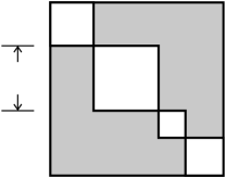
Figure 11. The area of the squares does not exceed the shaded area, if the side lengths are each at most half the total side length.

From Remark 10.4 we deduce that

$$\sum_{i\in{\mathscr{P}}}\lvert{w_{i}}\rvert^{2}\ \leqslant\ (1/2)\lvert{w}\rvert^{2}$$

and therefore

$$\sum_{(i,j)\in{\mathscr{I}}}\lvert{w_{i}}\rvert\lvert{w_{j}}\rvert\ \geqslant\ (1/2)\lvert{w}\rvert^{2}.$$

Finally, we have

$$\operatorname{Area}(wz^{-1})\ \leqslant\ 4C\lvert{w}\rvert^{2}\ \leqslant\ 8C\sum_{(i,j)\in{\mathscr{I}}}\lvert{w_{i}}\rvert\lvert{w_{j}}\rvert$$

so we are done by taking $K_{5}\geqslant 8C$.

Next consider the special case: $w_{i^{\prime}}$ is a word in $a_{\nu_{\ell}},b_{\nu_{\ell}}$ and $\lvert{w_{i^{\prime}}}\rvert>(1/2)\lvert{w}\rvert$. Write $w=w_{L}w_{i^{\prime}}w_{R}$, so that $\lvert{w_{L}}\rvert+\lvert{w_{R}}\rvert<\lvert{w_{i^{\prime}}}\rvert$. Note that it will suffice for us to prove that $\operatorname{Area}(wz^{-1})\ \leqslant\ K_{5}\lvert{w_{i^{\prime}}}\rvert(\lvert{w_{L}}\rvert+\lvert{w_{R}}\rvert)$.

Let $\sigma$ and $\sigma^{\prime}$ be maximal segments in $\widehat{T}$ with common endpoint $v_{\nu_{\ell}}$, which diverge immediately. That is, their intersection consists of the single edge from the leaf $v_{\nu_{\ell}}$ to its parent vertex in $T$. This edge lies inside a triangle in the $(\lvert{T}\rvert+2)$–gon. Suppose without loss of generality that this triangle has index triple $(0,1,2)$ and that $A_{\nu_{\ell}}=A_{0}\subset F_{0}\times F_{1}$. The vertex group in $V_{T}$ corresponding to this triangle is $F_{0}\times F_{1}\times F_{2}$; denote this subgroup by $V$. For concreteness, suppose that $\sigma$ separates corner $0$ from corners $1$ and $2$, and $\sigma^{\prime}$ separates corner $1$ from corners $2$ and $0$.

We can express the $(\lvert{T}\rvert+2)$–gon as a union of two smaller sub-diagrams whose intersection is the $(0,1,2)$ triangle. Note that $\sigma$ and $\sigma^{\prime}$ each lie wholly inside one of these sub-diagrams. Thus $V_{T}$ has an expression as $A\ast_{V}B$ where $A$ is the fundamental group of the sub-diagram containing $\sigma$ and $B$ is the fundamental group of the sub-diagram containing $\sigma^{\prime}$. See Figure 12.

2pt * $=$ at 95 32 * $\cup$ at 178 32

${\sigma}$ [Br] at 6 18.5 ${\sigma}$ [tr] at 46 3.3 ${\sigma^{\prime}}$ [tl] at 49 6 ${\sigma^{\prime}}$ [Bl] at 74 15

${\sigma}$ [Br] at 112.5 20 ${\sigma}$ [t] at 154 3.5 ${\sigma^{\prime}}$ [t] at 205 6 ${\sigma^{\prime}}$ [l] at 230 19

* ${\color[rgb]{0,0,1}0}$ at 40.5 12 * ${\color[rgb]{0,0,1}1}$ at 55.5 12 * ${\color[rgb]{0,0,1}2}$ at 48 24

* ${\color[rgb]{0,0,1}0}$ at 147 12 * ${\color[rgb]{0,0,1}1}$ at 160 12 * ${\color[rgb]{0,0,1}2}$ at 154 24

* ${\color[rgb]{0,0,1}0}$ at 197 12 * ${\color[rgb]{0,0,1}1}$ at 209.5 12 * ${\color[rgb]{0,0,1}2}$ at 203.5 24

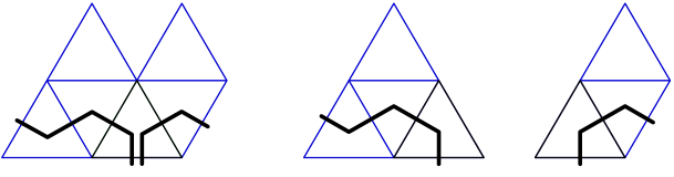
Figure 12. Expressing $V_{T}$ as $A\ast_{V}B$ with $S_{\sigma}\subset A$ and $S_{\sigma^{\prime}}\subset B$.

In particular, $S_{\sigma}\subset A$, $S_{\sigma^{\prime}}\subset B$, and $A\cap B=V$.

Let $\Delta$ be a reduced van Kampen diagram over $X_{T}$ with boundary $wz^{-1}$. Think of the boundary as being two arcs with the same endpoints, labeled by $w$ and $z$ respectively. Every edge along $w_{i^{\prime}}$ has a $\sigma$–corridor emanating from it. Since $w_{i^{\prime}}$ and $z$ are reduced words in $a_{\nu_{\ell}},b_{\nu_{\ell}}$, we can argue (as usual) that no $\sigma$–corridor has both ends on $w_{i^{\prime}}$ or on $z$, and that the $\sigma$–corridors emanating from $w_{i^{\prime}}$ and landing on $z$ all land on a connected subarc of the arc labeled $z$. The $\sigma$–corridors not landing on $z$ must land on $w_{L}$ or $w_{R}$, and one finds that these comprise at most $1/3$ of the corridors emanating from $w_{i^{\prime}}$ (because $\lvert{w_{i^{\prime}}}\rvert>\lvert{w_{L}}\rvert+\lvert{w_{R}}\rvert$).

Let $p_{1},p_{2}$ be the initial and final endpoints of the maximal segment along $w_{i^{\prime}}$ whose $\sigma$–corridors land on $z$. Let $q_{1},q_{2}$ be the analogous points along $z$, so that $p_{i}$ is joined to $q_{i}$ by the side of a $\sigma$–corridor ($i=1,2$). Note that the subsegments $[p_{1},p_{2}]$ and $[q_{1},q_{2}]$ are labeled by the same word in $a_{\nu_{\ell}},b_{\nu_{\ell}}$, by Remark 6.3.

In a similar fashion, there are $\sigma^{\prime}$–corridors emanating from $w_{i^{\prime}}$, at least 2/3 of which land on a connected subsegment of $z$. Define $p_{1}^{\prime}$, $p_{2}^{\prime}$, $q_{1}^{\prime}$, $q_{2}^{\prime}$ analogously to $p_{1}$, $p_{2}$, $q_{1}$, and $q_{2}$.

Now let $[p_{i},q_{i}]$ denote the side of the $\sigma$–corridor joining $p_{i}$ to $q_{i}$ ($i=1,2$). Define $[p_{i}^{\prime},q_{i}^{\prime}]$ analogously. Note that the label along $[p_{1},q_{1}]$ represents an element of $S_{\sigma}\subset A$. However, $p_{1}$ and $q_{1}$ are also joined by the path $[p_{1},p_{1}^{\prime}]\cdot[p_{1}^{\prime},q_{1}^{\prime}]\cdot[q_{1}^{\prime},q_{1}]$ where the first and third segments run along $w_{i^{\prime}}$ and $z$ respectively. This path represents an element of $B$. Therefore, $[p_{1},q_{1}]$ represents an element of $A\cap B=V$. By Lemma 10.1 we have $S_{\sigma}\cap V=F_{1}\times F_{2}$, and so $[p_{1},q_{1}]$ in fact represents an element of this latter subgroup. By the same argument, $[p_{2},q_{2}]$ also represents an element of $F_{1}\times F_{2}$.

We need to introduce a little more notation. Let $\alpha$ be the path along the boundary of $\Delta$ from $q_{1}$ to $p_{1}$ which contains the segment labeled $w_{L}$. Similarly, let $\beta$ be the path in the boundary from $p_{2}$ to $q_{2}$ which contains $w_{R}$. Let $p_{0},p_{3}$ be the initial and final endpoints of the segment labeled $w_{i^{\prime}}$. Let $q_{0},q_{3}$ be the endpoints of the segment labeled $z$. Note that $\lvert{[p_{0},p_{1}]}\rvert\leqslant\lvert{w_{L}}\rvert$ since the $\sigma$–corridors from $[p_{0},p_{1}]$ land on $w_{L}$. Similarly, $\lvert{[p_{2},p_{3}]}\rvert\leqslant\lvert{w_{R}}\rvert$. Because $\lvert{z}\rvert\leqslant\lvert{w}\rvert$, we have

$$\lvert{[q_{0},q_{1}]}\rvert+\lvert{[q_{2},q_{3}]}\rvert\ \leqslant\ \lvert{w_{L}}\rvert+\lvert{[p_{0},p_{1}]}\rvert+\lvert{[p_{2},p_{3}]}\rvert+\lvert{w_{R}}\rvert$$

$$\leqslant\ 2(\lvert{w_{L}}\rvert+\lvert{w_{R}}\rvert)$$

and therefore

$$\lvert{\alpha}\rvert+\lvert{\beta}\rvert\ \leqslant\ 4(\lvert{w_{L}}\rvert+\lvert{w_{R}}\rvert).$$ (10.6)

At this point we discard the diagram $\Delta$ and start over with its boundary loop. We have seen that $\alpha$ and $\beta$ represent elements $g_{\alpha}$ and $g_{\beta}$ of the subgroup $F_{1}\times F_{2}\subset V$. Attach a segment $[q_{1},p_{1}]$ to the points $q_{1}$ and $p_{1}$, and label it by a reduced word representing $g_{\alpha}$, of the form $u(x_{1},y_{1})v(x_{2},y_{2})$. Similarly, attach a segment $[q_{2},p_{2}]$ labeled by a reduced word $u^{\prime}(x_{1},y_{1})v^{\prime}(x_{2},y_{2})$ representing $g_{\beta}^{-1}$ to the points $q_{2}$ and $p_{2}$. Note that the loop $[p_{1},p_{2}]\cdot[p_{2},q_{2}]\cdot[q_{2},q_{1}]\cdot[q_{1},p_{1}]$ is labeled by generators of $V$, and the only occurrences of generators of $F_{2}$ are in the reduced words $v$ and $v^{\prime}$. It follows that $v=v^{\prime}$.

Now define $o_{1}$ to be the point along $[q_{1},p_{1}]$ such that $[q_{1},o_{1}]$ is labeled by $u(x_{1},y_{1})$ and $[o_{1},p_{1}]$ is labeled by $v(x_{2},y_{2})$. Similarly let $o_{2}$ be the point on $[q_{2},p_{2}]$ such that $[q_{2},o_{2}]$ is labeled by $u^{\prime}(x_{1},y_{1})$ and $[o_{2},p_{2}]$ is labeled by $v(x_{2},y_{2})$. Attach one more segment $[o_{1},o_{2}]$ to the points $o_{1}$ and $o_{2}$, labeled by the same word in $a_{0},b_{0}$ ($=a_{\nu_{\ell}},b_{\nu_{\ell}}$) as $[p_{1},p_{2}]$ and $[q_{1},q_{2}]$.

We proceed now to fill the original boundary loop with a van Kampen diagram, in four parts. Fill the loop $\alpha\cdot[p_{1},q_{1}]$ with a least-area van Kampen diagram $\Delta_{\alpha}$ over $X_{T}$. Fill $\beta\cdot[q_{2},p_{2}]$ with a least-area diagram $\Delta_{\beta}$ over $X_{T}$. To estimate the areas of $\Delta_{\alpha}$ and $\Delta_{\beta}$, choose a segment $\sigma^{\prime\prime}\subset\widehat{T}$ which passes through the $(0,1,2)$ triangle and separates corner $2$ from corners $0$ and $1$. Note that $x_{1},y_{1}\in{\mathscr{S}}_{\sigma^{\prime}}-{\mathscr{S}}_{\sigma^{\prime\prime}}$ and $x_{2},y_{2}\in{\mathscr{S}}_{\sigma^{\prime\prime}}-{\mathscr{S}}_{\sigma^{\prime}}$. Every edge along $[p_{1},q_{1}]$ has either a $\sigma^{\prime}$–corridor or a $\sigma^{\prime\prime}$–corridor in $\Delta_{\alpha}$ emanating from it, and not both. Since the words $u(x_{1},y_{1})$, $v(x_{2},y_{2})$ are reduced, these corridors can only land on $\alpha$. It follows that

$$\lvert{[p_{1},q_{1}]}\rvert\ \leqslant\ 2\lvert{\alpha}\rvert.$$ (10.7)

By a similar argument using $\Delta_{\beta}$, we have

$$\lvert{[p_{2},q_{2}]}\rvert\ \leqslant\ 2\lvert{\beta}\rvert.$$ (10.8)

From (10.7) and (10.8) we deduce that

$$\operatorname{Area}(\Delta_{\alpha})\ \leqslant\ C(3\lvert{\alpha}\rvert)^{2}\ \text{ and }\ \operatorname{Area}(\Delta_{\beta})\ \leqslant\ C(3\lvert{\beta}\rvert)^{2}.$$

Two more loops remain to be filled. Let $\hat{w}(a_{0},b_{0})$ be the word labeling $[p_{1},p_{2}]$ and $[o_{1},o_{2}]$. The loop $[p_{1},p_{2}]\cdot[p_{2},o_{2}]\cdot[o_{2},o_{1}]\cdot[o_{1},p_{1}]$ is labeled by the commutator $[\hat{w}(a_{0},b_{0}),v(x_{2},y_{2})]$. Adjoin a triangular relator to each edge of $[p_{1},p_{2}]$ and $[o_{1},o_{2}]$ to obtain paths labeled by the word $\hat{w}(\overline{x}_{0}x_{1},\overline{y}_{0}y_{1})$. Now these paths and the paths $[p_{1},o_{1}]$, $[p_{2},o_{2}]$ can be filled using commutator relators. In this way the loop $[p_{1},p_{2}]\cdot[p_{2},o_{2}]\cdot[o_{2},o_{1}]\cdot[o_{1},p_{1}]$ bounds a diagram $\Delta_{012}$ over $X_{T}$ of area $2\lvert{[p_{1},p_{2}]}\rvert+2(2\lvert{[p_{1},p_{2}]}\rvert)\lvert{v}\rvert$.

Finally consider the loop $[o_{1},o_{2}]\cdot[o_{2},q_{2}]\cdot[q_{2},q_{1}]\cdot[q_{1},o_{1}]$. It is labeled entirely by generators of $F_{0}\times F_{1}$ and represents the trivial element, so it bounds a least-area diagram $\Delta_{01}$ over $X_{01}$. Its boundary is labeled by the word

$$\hat{w}(a_{0},b_{0})u^{\prime}(x_{1},y_{1})^{-1}\hat{w}(a_{0},b_{0})^{-1}u(x_{1},y_{1})$$

with each of the four subwords being reduced. Consider corridors in $\Delta_{01}$ for the corridor schemes ${\mathscr{S}}_{0}$ and ${\mathscr{S}}_{1}$. The ${\mathscr{S}}_{0}$–corridors can only land on the sides $[q_{1},q_{2}]$ and $[o_{1},o_{2}]$, and since these sides are labeled by reduced words, each such corridor has one end on each side. Thus, each edge of $[q_{1},q_{2}]$ is joined by an ${\mathscr{S}}_{0}$–corridor to the edge of $[o_{1},o_{2}]$ corresponding to the same letter of $\hat{w}$.

Consider the arrangement of the ${\mathscr{S}}_{1}$–corridors in $\Delta_{01}$. Every edge in the boundary has an ${\mathscr{S}}_{1}$–corridor emanating from it. There are no corridors of annulus type (see Remarks 10.2), and corridors cannot join two edges in the same side of the boundary. If there is a corridor joining $[q_{1},o_{1}]$ to $[q_{2},o_{2}]$ then we must have

$$2\lvert{[p_{1},p_{2}]}\rvert\ \leqslant\ \lvert{[q_{1},o_{1}]}\rvert+\lvert{[q_{2},o_{2}]}\rvert$$ (10.9)

and we will be satisfied for the moment. Assume now that no such corridor is present. Then, the most general arrangement is shown in Figure 13.

2pt * $m$ at 24 6 $o_{1}$ [r] at 0 60 $q_{1}$ [r] at .5 14 $o_{2}$ [l] at 128.5 65 $q_{2}$ [l] at 127 1

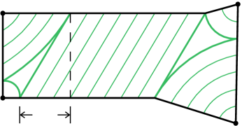
Figure 13. A generic configuration of ${\mathscr{S}}_{1}$–corridors in $\Delta_{01}$.

Notice that corridors running between $[o_{1},o_{2}]$ and $[q_{1},q_{2}]$ will land on edges that are offset by a fixed amount $m\leqslant\min\{\lvert{[q_{1},o_{1}]}\rvert,\lvert{[q_{2},o_{2}]}\rvert\}$. In particular an ${\mathscr{S}}_{0}$–corridor can be crossed by at most $m+1$ ${\mathscr{S}}_{1}$–corridors of this type. There are $\lvert{[q_{1},o_{1}]}\rvert+\lvert{[q_{2},o_{2}]}\rvert$ ${\mathscr{S}}_{1}$–corridors not of this type, so an ${\mathscr{S}}_{0}$–corridor can cross no more than $2(\lvert{[q_{1},o_{1}]}\rvert+\lvert{[q_{2},o_{2}]}\rvert)$ ${\mathscr{S}}_{1}$–corridors overall.

By Remarks 10.2, an ${\mathscr{S}}_{0}$–corridor and an ${\mathscr{S}}_{1}$–corridor will intersect if and only if their endpoints are linked (or equal) in the boundary of $\Delta_{01}$, and when this occurs, the intersection will have area $1$ or $2$. Moreover, every $2$–cell of $\Delta_{01}$ is in the intersection of such a pair. Since every ${\mathscr{S}}_{0}$–corridor is crossed by at most $2(\lvert{[q_{1},o_{1}]}\rvert+\lvert{[q_{2},o_{2}]}\rvert)$ ${\mathscr{S}}_{1}$–corridors, we conclude that

$$\operatorname{Area}(\Delta_{01})\leqslant 4(\lvert{[q_{1},o_{1}]}\rvert+\lvert{[q_{2},o_{2}]}\rvert)\lvert{[o_{1},o_{2}]}\rvert.$$

To finish, first suppose we are in the special case where (10.9) holds. Then, the total perimeter is at most $12(\lvert{w_{L}}\rvert+\lvert{w_{R}}\rvert)$ by (10.7), (10.8), and (10.6). Then

$$\operatorname{Area}(wz^{-1})\ \leqslant\ C(12(\lvert{w_{L}}\rvert+\lvert{w_{R}}\rvert))^{2}\ \leqslant\ 144C\lvert{w_{i^{\prime}}}\rvert(\lvert{w_{L}}\rvert+\lvert{w_{R}}\rvert)$$

so we require $K_{5}\geqslant 144C$ to cover this case.

Otherwise, we use our estimates for the areas of the four diagrams $\Delta_{\alpha}$, $\Delta_{\beta}$, $\Delta_{012}$, and $\Delta_{01}$. Since $\lvert{[p_{1},p_{2}]}\rvert=\lvert{[o_{1},o_{2}]}\rvert=\lvert{[q_{1},q_{2}]}\rvert\leqslant\lvert{w_{i^{\prime}}}\rvert$, these estimates yield

$$\operatorname{Area}(wz^{-1})\ \leqslant\ 9C\lvert{\alpha}\rvert^{2}+9C\lvert{\beta}\rvert^{2}+(2\lvert{w_{i^{\prime}}}\rvert+4\lvert{w_{i^{\prime}}}\rvert\lvert{v}\rvert)+4(\lvert{u}\rvert+\lvert{u^{\prime}}\rvert)\lvert{w_{i^{\prime}}}\rvert.$$

Using (10.7) and (10.8) this reduces to

$$\operatorname{Area}(wz^{-1})\ \leqslant\ 9C(\lvert{\alpha}\rvert+\lvert{\beta}\rvert)^{2}+\lvert{w_{i^{\prime}}}\rvert(2+8(\lvert{\alpha}\rvert+\lvert{\beta}\rvert)).$$

Note that $(\lvert{\alpha}\rvert+\lvert{\beta}\rvert)\leqslant 4\lvert{w_{i^{\prime}}}\rvert$ by (10.6), and a further application of (10.6) yields the following:

$$\operatorname{Area}(wz^{-1})\ \leqslant\ 36C\lvert{w_{i^{\prime}}}\rvert(\lvert{\alpha}\rvert+\lvert{\beta}\rvert)+\lvert{w_{i^{\prime}}}\rvert(2+8(\lvert{\alpha}\rvert+\lvert{\beta}\rvert))$$

$$\leqslant\ (36C+10)\lvert{w_{i^{\prime}}}\rvert(\lvert{\alpha}\rvert+\lvert{\beta}\rvert)$$

$$\leqslant\ (144C+40)\lvert{w_{i^{\prime}}}\rvert(\lvert{w_{L}}\rvert+\lvert{w_{R}}\rvert).$$

Taking $K_{5}\geqslant 144C+40$ completes the proof. ∎

Proposition 10.10 (Area in $S_{T,n}$).

Given $T$ and $n$ there is a constant $K_{6}$ with the following property. Suppose $w$ and $z(a_{\nu_{j}},b_{\nu_{j}})$ represent the same element of $A_{\nu_{j}}\subset S_{T,n}$, where $w$ is a word in the standard generators of $S_{T,n}$ and $z$ is reduced. Then $\operatorname{Area}(wz^{-1})\ \leqslant\ K_{6}\lvert{w}\rvert^{2\alpha}$.

We follow the proof of Proposition 5.5 in [BBFS09].

Proof.

The proof is by induction on $\lvert{w}\rvert$. Let $M=\max\{\lvert{\varphi^{n}(x)}\rvert,\lvert{\varphi^{n}(y)}\rvert,\lvert{\varphi^{-n}(x)}\rvert,\lvert{\varphi^{-n}(y)}\rvert\}$. Let $K_{6}=M^{2}K_{4}^{2}K_{5}$, where $K_{4}$ is given by Corollary 9.14 and $K_{5}$ is given by Proposition 10.3. Write $w$ as $w_{1}\dotsc w_{k}$ where each $w_{i}$ either is a word in the standard generators of $V_{T}$, or $w_{i}=r_{j}^{\pm 1}u_{i}r_{j}^{\mp 1}$ for some $j$. Let $I_{r}$ be the set of indices for which the latter case occurs, and note that $w_{i}$ represents an element of a peripheral subgroup of $V_{T}$. Let $v_{i}$ be the reduced word in the generators of that subgroup representing $w_{i}$. For $i\not\in I_{r}$ let $v_{i}=w_{i}$, and define $v=v_{1}\dotsm v_{k}$.

By Proposition 10.3 we have $\operatorname{Area}(vz^{-1})\leqslant K_{5}\sum_{(i,j)\in{\mathscr{I}}}\lvert{v_{i}}\rvert\lvert{v_{j}}\rvert$. For $i\in I_{r}$ we have either $\lvert{v_{i}}\rvert\leqslant K_{4}\lvert{w_{i}}\rvert^{\alpha}$ (if $v_{i}\in A_{\nu_{0}}$) or $\lvert{v_{i}}\rvert\leqslant MK_{4}\lvert{u_{i}}\rvert^{\alpha}$ (if $u_{i}\in A_{\nu_{0}}$), by Corollary 9.14. In any case (including $i\not\in I_{r})$ we have $\lvert{v_{i}}\rvert\leqslant MK_{4}\lvert{w_{i}}\rvert^{\alpha}$. Therefore,

$$\operatorname{Area}(vz^{-1})\ \leqslant\ K_{6}\sum_{(i,j)\in{\mathscr{I}}}\lvert{w_{i}}\rvert^{\alpha}\lvert{w_{j}}\rvert^{\alpha}.$$ (10.11)

Next note that

$$\operatorname{Area}(wv^{-1})\ \leqslant\ \sum_{i\in I_{r}}\operatorname{Area}(w_{i}v_{i}^{-1})$$

since $w_{i}=v_{i}$ for $i\not\in I_{r}$. For each term $\operatorname{Area}(w_{i}v_{i}^{-1})$, recall that $w_{i}=r_{j}^{\pm 1}u_{i}r_{j}^{\mp 1}$. Let $z_{i}$ be the reduced word in peripheral generators representing the same peripheral element as $u_{i}$. Apply the induction hypothesis to $u_{i}$ to obtain

$$\operatorname{Area}(u_{i}z_{i}^{-1})\ \leqslant\ K_{6}\lvert{u_{i}}\rvert^{2\alpha}\ =\ K_{6}(\lvert{w_{i}}\rvert-2)^{2\alpha}.$$ (10.12)

One of the words $z_{i},v_{i}$ is an element of $A_{\nu_{0}}$, so there is a folded $r_{j}$–corridor with boundary word $r_{j}^{\pm 1}z_{i}r_{j}^{\mp 1}v_{i}^{-1}$, where one of the boundary arcs labeled $z_{i}$ or $v_{i}$ is the bottom and the other is the top. The area of this corridor is the length of the bottom, which is at most $M\lvert{v_{i}}\rvert$. As noted above, $\lvert{v_{i}}\rvert\leqslant MK_{4}\lvert{w_{i}}\rvert^{\alpha}$, and so

$$\operatorname{Area}(r_{j}^{\pm 1}z_{i}r_{j}^{\mp 1}v_{i}^{-1})\ \leqslant\ MK_{4}\lvert{w_{i}}\rvert^{\alpha}.$$

Together with (10.12) we obtain

$$\operatorname{Area}(w_{i}v_{i}^{-1})\ \leqslant\ K_{6}((\lvert{w_{i}}\rvert-2)^{2\alpha}+\lvert{w_{i}}\rvert^{\alpha})$$

$$\leqslant\ K_{6}\lvert{w_{i}}\rvert^{2\alpha}$$ (10.13)

for $i\in I_{r}$. The last inequality above holds exactly as in [BBFS09, Proposition 5.5]: for numbers $x\geqslant 0$ one has $(x+2)^{2\alpha}\geqslant x^{\alpha}(x+2)^{\alpha}+2^{\alpha}(x+2)^{\alpha}\geqslant x^{2\alpha}+(x+2)^{\alpha}$.

Lastly, add together (10.11) and (10) for each $i\in I_{r}$ to obtain

$$\operatorname{Area}(wz^{-1})\ \leqslant\ K_{6}\sum_{(i,j)\in{\mathscr{I}}}\lvert{w_{i}}\rvert^{\alpha}\lvert{w_{j}}\rvert^{\alpha}\ +\ K_{6}\sum_{i\in I_{r}}\lvert{w_{i}}\rvert^{2\alpha}$$

$$\leqslant\ K_{6}\sum_{i\not=j}\lvert{w_{i}}\rvert^{\alpha}\lvert{w_{j}}\rvert^{\alpha}\ +\ K_{6}\sum_{i}\lvert{w_{i}}\rvert^{2\alpha}.$$

The latter quantity is $K_{6}\lvert{w}\rvert^{2\alpha}$, as desired. ∎

Theorem 10.14.

Given $T$ and $n$ let $m=\lvert{T}\rvert+1$, let $\lambda>1$ be the Perron-Frobenius eigenvalue of $\varphi$, and let $\alpha=n\log_{m}(\lambda)$. If $\alpha\geqslant 1$ then the Dehn function of $S_{T,n}$ is given by $\delta(x)=x^{2\alpha}$.

Proof.

First we establish the lower bound $\delta(x)\succcurlyeq x^{2\alpha}$. Let $w(x,y)$ be a monotone palindromic word (eg. $x$) and consider the snowflake diagrams $\Delta(w,i)$ for $i\geqslant 1$. Let $n_{i}$ be the boundary length of $\Delta(w,i)$. The boundary word has $4m^{i-1}$ occurrences of the letters $r_{j}$ in it, and two adjacent such letters are never separated by more than $m\lvert{w}\rvert$ letters from $V_{T}$. Thus we have

$$4m^{i-1}\ \leqslant\ n_{i}\ \leqslant\ 4(m\lvert{w}\rvert+1)m^{i-1}.$$ (10.15)

From the second of these inequalities we obtain

$$(n_{i})^{\alpha}\ \leqslant\ \left(\frac{4(m\lvert{w}\rvert+1)}{m}\right)^{\alpha}(m^{\alpha})^{i}$$

$$=\ \left(\frac{4(m\lvert{w}\rvert+1)}{m}\right)^{\alpha}\lambda^{ni}$$

and so

$$\left(\frac{m}{4(m\lvert{w}\rvert+1)}\right)^{\alpha}(n_{i})^{\alpha}\ \leqslant\ \lambda^{ni}.$$

Next, $\Delta(w,i)$ has area at least $6\lvert{T}\rvert\lvert{\varphi^{in}(w)}\rvert^{2}$, which is the area of the doubled canonical diagram at its center. There is a constant $C$ such that $\lvert{\varphi^{k}(v)}\rvert\geqslant C\lambda^{k}\lvert{v}\rvert$ for every non-trivial word $v$. Thus,

$$\operatorname{Area}(\Delta(w,i))\ \geqslant\ 6\lvert{T}\rvert C^{2}\lvert{w}\rvert^{2}\bigl{(}\lambda^{ni}\bigr{)}^{2}$$

$$\geqslant\ 6\lvert{T}\rvert C^{2}\lvert{w}\rvert^{2}\left(\frac{m}{4(m\lvert{w}\rvert+1)}\right)^{2\alpha}(n_{i})^{2\alpha}.$$

Taking $D=6\lvert{T}\rvert C^{2}\lvert{w}\rvert^{2}\left(\frac{m}{4(m\lvert{w}\rvert+1)}\right)^{2\alpha}$, we have shown that $\delta_{Y_{T,n}}(n_{i})\geqslant D(n_{i})^{2\alpha}$ for each $i$, because $\Delta(w,i)$ is a least-area diagram over $Y_{T,n}$ with boundary length $n_{i}$. By (10.15) the ratios $n_{i+1}/n_{i}$ are bounded, and so we conclude by Remark 2.1 that $\delta(x)\succcurlyeq x^{2\alpha}$.

The upper bound follows immediately from Proposition 10.10: taking $z$ to be the empty word, $\operatorname{Area}(w)\leqslant K_{6}\lvert{w}\rvert^{2\alpha}$ for every word $w$ representing the trivial element of $S_{T,n}$. Thus $\delta(x)\preccurlyeq x^{2\alpha}$. ∎

References

- [ABD+13] Aaron Abrams, Noel Brady, Pallavi Dani, Moon Duchin, and Robert Young, Pushing fillings in right-angled Artin groups, J. Lond. Math. Soc. (2) 87 (2013), no. 3, 663–688. MR 3073670
- [ABDY13] Aaron Abrams, Noel Brady, Pallavi Dani, and Robert Young, Homological and homotopical Dehn functions are different, Proc. Natl. Acad. Sci. USA 110 (2013), no. 48, 19206–19212. MR 3153947
- [Bas93] Hyman Bass, Covering theory for graphs of groups, J. Pure Appl. Algebra 89 (1993), no. 1-2, 3–47. MR 1239551 (94j:20028)
- [BB00] N. Brady and M. R. Bridson, There is only one gap in the isoperimetric spectrum, Geom. Funct. Anal. 10 (2000), no. 5, 1053–1070. MR 1800063 (2001j:20046)
- [BBFS09] Noel Brady, Martin R. Bridson, Max Forester, and Krishnan Shankar, Snowflake groups, Perron-Frobenius eigenvalues and isoperimetric spectra, Geom. Topol. 13 (2009), no. 1, 141–187. MR 2469516 (2010a:20090)
- [BBMS97] Gilbert Baumslag, Martin R. Bridson, Charles F. Miller, III, and Hamish Short, Finitely presented subgroups of automatic groups and their isoperimetric functions, J. London Math. Soc. (2) 56 (1997), no. 2, 292–304. MR 1489138 (98j:20034)
- [BBMS00] by same author, Fibre products, non-positive curvature, and decision problems, Comment. Math. Helv. 75 (2000), no. 3, 457–477. MR 1793798 (2001k:20091)
- [BCD08] Noel Brady, Matt Clay, and Pallavi Dani, Morse theory and conjugacy classes of finite subgroups, Geom. Dedicata 135 (2008), 15–22. MR 2413325 (2009d:20103)
- [BG10] Martin R. Bridson and Daniel Groves, The quadratic isoperimetric inequality for mapping tori of free group automorphisms, Mem. Amer. Math. Soc. 203 (2010), no. 955, xii+152. MR 2590896 (2011g:20058)
- [BGL11] Noel Brady, Dan P. Guralnik, and Sang Rae Lee, Dehn functions and finiteness properties of subgroups of perturbed right-angled Artin groups, preprint, http://arxiv.org/abs/1102.5551, 2011.
- [BH99] Martin R. Bridson and André Haefliger, Metric spaces of non-positive curvature, Grundlehren der Mathematischen Wissenschaften [Fundamental Principles of Mathematical Sciences], vol. 319, Springer-Verlag, Berlin, 1999. MR 1744486 (2000k:53038)
- [Bra95] Thomas Brady, Complexes of nonpositive curvature for extensions of by , Topology Appl. 63 (1995), no. 3, 267–275. MR 1334311 (96e:20056)
- [Bri02] Martin R. Bridson, The geometry of the word problem, Invitations to geometry and topology, Oxf. Grad. Texts Math., vol. 7, Oxford Univ. Press, Oxford, 2002, pp. 29–91. MR 1967746 (2004g:20056)
- [Bri13] by same author, On the subgroups of right-angled Artin groups and mapping class groups, Math. Res. Lett. 20 (2013), no. 2, 203–212. MR 3151642
- [BRS07] Noel Brady, Tim Riley, and Hamish Short, The geometry of the word problem for finitely generated groups, Advanced Courses in Mathematics. CRM Barcelona, Birkhäuser Verlag, Basel, 2007, Papers from the Advanced Course held in Barcelona, July 5–15, 2005. MR 2281936 (2009j:20053)
- [DR13] Will Dison and Timothy R. Riley, Hydra groups, Comment. Math. Helv. 88 (2013), no. 3, 507–540. MR 3093501
- [FM91] Mark Feighn and Geoffrey Mess, Conjugacy classes of finite subgroups of Kleinian groups, Amer. J. Math. 113 (1991), no. 1, 179–188. MR 1087807 (92a:57042)
- [Ger98] S. M. Gersten, Cohomological lower bounds for isoperimetric functions on groups, Topology 37 (1998), no. 5, 1031–1072. MR 1650363 (2000c:20063)
- [LN03] Ian J. Leary and Brita E. A. Nucinkis, Some groups of type , Invent. Math. 151 (2003), no. 1, 135–165. MR 1943744 (2003k:20086)
- [SBR02] Mark V. Sapir, Jean-Camille Birget, and Eliyahu Rips, Isoperimetric and isodiametric functions of groups, Ann. of Math. (2) 156 (2002), no. 2, 345–466. MR 1933723 (2005b:20077a)