Cortical Computation via Iterative Constructions
Abstract
We study Boolean functions of an arbitrary number of input variables that can be realized by simple iterative constructions based on constant-size primitives. This restricted type of construction needs little global coordination or control and thus is a candidate for neurally feasible computation. Valiant’s construction of a majority function can be realized in this manner and, as we show, can be generalized to any uniform threshold function. We study the rate of convergence, finding that while linear convergence to the correct function can be achieved for any threshold using a fixed set of primitives, for quadratic convergence, the size of the primitives must grow as the threshold approaches or . We also study finite realizations of this process and the learnability of the functions realized. We show that the constructions realized are accurate outside a small interval near the target threshold, where the size of the construction grows as the inverse square of the interval width. This phenomenon, that errors are higher closer to thresholds (and thresholds closer to the boundary are harder to represent), is a well-known cognitive finding.
1 Introduction
Cortical computation.
Among the many unexplained abilities of the cortex are learning complex patterns and invariants from relatively few examples. This is manifested in a range of cognitive functions including visual and auditory categorization, motor learning and language. In spite of the highly varied perceptual and cognitive tasks accomplished, the substrate appears to be relatively uniform in the distribution and type of cells. How could these billion cells organize themselves so effectively?
Cortical computation must therefore be highly distributed, require little synchrony (number of pairs of events that must happen in lock-step across neurons), little global control (longest chain of events that must happen in sequence) and be based on very simple primitives [Papadimitriou and Vempala, 2015b]. Assuming that external stimuli are parsed as sets of binary sensory features, our central question is the following:
What functions can be represented and learned by algorithms so simple that one could imagine them happening in the cortex?
Perhaps the most natural primitives are the AND and OR functions on two input variables. These functions are arguably neurally plausible. They were studied as JOIN and LINK by Valiant [1994, 2000, 2005], Feldman and Valiant [2009], who showed how to implement them in the neuroidal model. An item is a collection of neurons (corresponding to a neural assembly in neuroscience) that represents some learned or sensed concept. Given two items , the JOIN operation forms a new item , which “fires” when both and fire, i.e., represents . captures association, and causes to fire whenever fires. By setting and , we achieve that is effectively . While the precise implementation and neural correlates of JOIN and LINK are unclear, there is evidence that the brain routinely engages in hierarchical memory formation.
Monotone Boolean functions.
Functions constructed by recursive processes based on AND/OR trees have been widely studied in the literature, motivated by the design of reliable circuits as in [Moore and Shannon, 1956] and more recently, understanding the complexity-theoretic limitations of monotone Boolean functions. One line of work studies the set of functions that could be the limits of recursive processes, where at each step, the leaves of a tree are each replaced by constant-size functions. Moore and Shannon [1956], showed that a simple recursive construction leads to a threshold function, which can be applied to construct stable circuits. Valiant [1984] used their -variable primitive function to derive a small depth and size threshold function that evaluates to if at least fraction of the inputs are set to and to zero otherwise. The depth and size were and respectively. Calling it the amplification method, Boppana [1985] showed that Valiant’s construction is optimal. Dubiner and Zwick [1992] extended the lower bound to classes of read-once formulae. Hoory et al. [2006] gave smaller size Boolean circuits (where each gate can have fan out more than ), of size for the same threshold function. Luby et al. [1998] gave an alternative analysis of Valiant’s construction along with applications to coding. The construction of a Boolean formula was extended by Servedio [2004] to monotone linear threshold functions, in that they can be approximated on most inputs by monotone Boolean formulae of polynomial size. Friedman [1986] gave more efficient constructions for threshold functions with small thresholds.
Savicky gives conditions under which the limit of such a process is the uniform distribution on all Boolean functions with inputs [Savicky, 1987, 1990] (see also Brodsky and Pippenger [2005], Fournier et al. [2009]). In a different application, Goldman et al. [1993] showed how to use properties of these constructions to identify read-once formulae from their input-output behavior.
Our work.
Unlike previous work, where a single constant-sized function is chosen and applied recursively, we will allow constructions that randomly choose one of two constant-sized functions. To be neurally plausible, our constructions are bottom-up rather than top-down, i.e., at each step, we apply a constant-size function to an existing set of outputs. In addition, the algorithm itself must be very simple — our goal is not to find ways to realize all Boolean functions or to optimize the size of such realizations. Here we address the following questions: What functions of input items can be constructed in this iterative manner? Can arbitrary uniform threshold functions be realized? What size and depth of iterative constructions suffices to guarantee accurate computations? Can such functions and constructions be learned from examples, where the learning algorithm is also neurally plausible?
Our rationale for uniform threshold functions is two-fold. First, uniform threshold functions are fundamental in computer science and likely also for cognition. Second, the restriction to JOIN and LINK as primitives ensures that any resulting function will be monotone since negation is not possible in this framework. Moreover, if we require the construction to be symmetric, it would seem that the only obtainable family of Boolean functions are uniform thresholds. However, as we will see, there is a surprise here, and in fact we can get staircase functions, i.e., functions that take value on the interval where and .
To be able to describe our results precisely, we begin with a definition of iterative constructions.
1.1 Iterative constructions
A sequence of AND/OR operations can be represented as a tree. Such a tree with leaves naturally computes a function . We can build larger trees in a neurally plausible way by using a set of small AND/OR trees as building blocks. Let be a probability distribution on a finite set of trees. We define an iterative tree for as follows.
IterativeTree():
For each level from to , apply the following iteration times:
(level consists of the input items )
1.
Choose a tree according to .
2.
Choose items at random from the items on level .
3.
Build the tree with these items as leaves.
The construction of small AND/OR trees is a decentralized process requiring a short sequence of steps, i.e., the synchrony and control parameters are small. Therefore, we consider them to be neurally plausible.
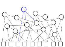
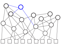
The iterative tree construction has a well-defined sequence of levels, with items from the next level having leaves only in the current level. A construction that needs even less coordination is the following: the probability that an item participates in future item creation decays exponentially with time. The weight of an item starts at when it is created and decays by a factor of each time unit. We refer to such constructions as exponential iterative constructions. An extreme version of this, which we call wild iterative construction, is to have , i.e, all items are equally likely to participate in the creation of new items. Figure 1 illustrates these constructions.
ExponentialConstruction():
Initialize the weights of input items to .
Construct items as follows:
1.
Choose a tree according to .
2.
Choose the leafs for independently from existing items with probability proportional to the weight of the item.
3.
Build the tree with these items as leaves.
4.
Multiply the weight of every item by .
1.2 Results
We are interested in the functions computed by high-level items of iterative constructions. In particular, we design iterative constructions so that high-level items compute a threshold function with high probability.
Definition 1.1.
The function is a -threshold if for and for .
For given probability distribution on a set of trees, the output of high-level items of a corresponding iterative construction depends on the following: the fraction of input items firing, the width of the levels, and the number of levels. For an item input, the fraction of input items firing must take the form , . Throughout the paper, we assume that the distance between the desired threshold and the fraction of input items firing is at least . To address , we first analyze the functions computed by high-level items of an iterative construction when the width of the levels is infinite, which is equivalent to the “top down” approach. Then in Section 5, we remove this assumption and analyze the “bottom-up” construction in which the items at level are fixed before the items at level are created. The following theorems give a guarantee on the probability that an iterative tree with infinite width levels accurately computes a threshold function in terms of the number of levels. To start, we restate Valiant’s result [Valiant, 1984]. Here is the golden ratio ().
Theorem 1.2.
Let be the tree that computes . Then, an item at level of an infinite width iteratively constructed tree for computes a -threshold function accurately with probability at least .
In this construction, the iterative tree that computes the threshold function is built using only one small tree. We show that it is possible to achieve arbitrary threshold functions if we allow our iterative tree to be built according to a probability distribution on two distinct smaller trees.
Theorem 1.3.
Let and let where is the tree that computes and is the tree that computes . Then, an item at level of an infinite width iteratively constructed tree for computes a -threshold function accurately with probability at least
The rate of convergence of this more general construction is linear rather than quadratic. While both are interesting, the latter allows us to guarantee a correct function on every input with depth only , since there are possible inputs.
Definition 1.4.
A construction exhibits linear convergence if items at level of an infinite width iterative tree accurately compute the threshold function with probability at least . A construction exhibits quadratic convergence if items at level of an infinite width iterative tree accurately compute the threshold function with probability at least .
The next theorem gives constructions using slightly larger trees with and leaves respectively (illustrated in Figure 2) that converge quadratically to a -threshold function for a range of values of , with more leaves giving a larger range. Moreover, these ranges are tight, i.e. no construction on trees with or leaves yields quadratic convergence to a -threshold function for outside these ranges.
Theorem 1.5.
(A) Let
and . Let be the probably distribution on trees in Figure 2. Then, an item at level of an infinite width iteratively constructed tree for computes a -threshold function accurately with probability at least . Moreover, for outside this range, there exists no such construction on trees with four leaves that converge quadratically to a -threshold function.
(B) Let and let be a value for which , so . Let be the probably distribution on trees in Figure 2. Then, an item at level of an infinite width iteratively constructed tree for computes a -threshold function accurately with probability at least . Moreover, for outside this range, there exists no such construction on trees with five leaves that converges quadratically to a -threshold function.
As the desired threshold approaches or , we show that an iterative tree that computes the -threshold function must use increasingly large trees as building blocks.
Theorem 1.6.
Let be a threshold, and let . Then, the construction of an iterative tree whose level items compute a -threshold function with probability at least must be defined over a probability distribution on trees with at least leaves.
This raises the question of whether it is possible to have quadratic convergence for any threshold. We can extend the constructions described in Theorem 1.5 by using analogous trees with six and seven leaves to obtain quadratic convergence for thresholds in the ranges and respectively. However, it is not possible to generalize this construction beyond this point, as we discuss in Section 4. Instead, to achieve quadratic convergence for thresholds near the boundaries, we turn to the following construction, which asymptotically matches the lower bound of Theorem 1.6. We define as a tree on leaves that computes and as a tree on leaves that computes .
Theorem 1.7.
For any , there exists and a probability distribution on and that yields an iterative tree with quadratic convergence to a -threshold function. Similarly for any , there exists and a probability distribution on and that yields an iterative tree with quadratic convergence to a -threshold function.
There is a trade-off between constructing iterative trees that converge faster and requiring minimal coordination in order to build the subtrees. Building a specified tree on a small number of leaves requires less coordination than building a specified tree on many leaves. Therefore, as approaches or , constructing an iterative tree with quadratic convergence becomes less neurally plausible because the construction of each subtree requires much coordination. These results are in line with behavioral findings [Rosch et al., 1976, Rosch, 1978] and computational models [Arriaga and Vempala, 2006, Arriaga et al., 2015] about categorization being easier when concepts are more robust.
In Section 4, we characterize the class of functions that can be achieved by iterative constructions allowing building block trees of any size. We show that it is possible to achieve an arbitrarily close approximation of any staircase function in which each step intersects the line . This result is described more precisely in Theorem 4.10.
In the following section we turn to finite realizations of iterative trees. The above theorems analyze the behavior of an iterative construction where the width of the levels is infinite. We assumed that for any input the number of items turned on at given level of the tree is equal to its expectation. Imagining a “bottom up” construction, we note that the chance that the number of items firing at a given level deviates from expectation is non-trivial. Such deviations percolate up the tree and effect the probability that high-level items compute the threshold function accurately. The smaller the width of a level, the more likely that the number of items on at that level deviates significantly from expectation, rendering the tree less accurate. How large do the levels of an iteratively constructed tree need to be in order to ensure a reasonable degree of accuracy?
Theorem 1.8.
Consider a construction of a -threshold function with quadratic convergence described in Theorem 1.5 or Theorem 1.7 in which each level has items and the fraction of input items firing is at least from the threshold . Then, with probability at least , items at level will accurately compute the threshold function for and .
As a direct corollary, by setting and , we realize a -threshold construction of size for any , matching the best-known construction which was for a specific threshold [Hoory et al., 2006]. The finite-width version of Theorem 1.3 is given in Section 5.
The exponential iterative construction also converges to a -threshold function for appropriate . We give the statements here for the wild iterative construction (with no weight decay) and the general exponential construction.
Theorem 1.9.
Consider a wild construction on inputs for the -threshold function given in Theorem 1.3 in which where is the distance between and the fraction of inputs firing. Then, there is an absolute constant such that for , the item accurately computes the -threshold function with probability at least .
Theorem 1.10.
Consider an exponential construction on inputs for the -threshold function given in Theorem 1.3 in which and Then for
with probability at least , the item will compute the -threshold function.
Finally, in Section 6, we give a simple cortical algorithm to learn a uniform threshold function from a single example, described more precisely by the following theorem.
Theorem 1.11.
Let such that , , and . Then, on any input in which the fraction of input items firing is outside , items at level of an iterative tree produced by LearnThreshold() will compute a -threshold function with probability at least .
2 Polynomials of AND/OR Trees
Let be the Boolean function computed by an AND/OR tree with leaves. We define as the probability that evaluates to if each input item is independently set to with probability .
We analogously define for probability distributions on trees; let be the probability that a tree chosen according to evaluates to 1 if each input item is independently set to with probability . Let be the probability of in distribution . We have
In an iterative construction for the probability distribution , an item at level evaluates to 1 with probability where is the probability that an item at level evaluates to . In the case where the width of the levels is infinite, the fraction of inputs firing any level is exactly equal its expectation. Therefore, the probability that items at level evaluate to 1 is where is the probability an input is set to 1. This follows directly from the recurrence relation:
In the remainder of this section, we collect properties of polynomials of AND/OR trees to be used in the analysis of iterative trees.
We call a polynomial achievable if it can be written as for some AND/OR tree . We call a polynomial achievable through convex combinations if it can be written as for some probability distribution on AND/OR trees . Table 1 lists all achievable polynomials with degree at most five. Note that is closed under the AND and OR operations. If , then and . The set of polynomials achievable through convex combinations is the convex hull of .
Lemma 2.1.
Let be the set of achievable polynomials. Let be a polynomial in . Then,
-
1.
-
2.
-
3.
-
4.
If has degree , then is the polynomial for a tree on leaves.
Proof.
We proceed by induction on the degree of . For , is the only polynomial in and all the above properties hold. Next assume all the properties hold for polynomials of degree less than . Let be an achievable polynomial of degree . Then the root of the tree for , which we call , is either an AND or an OR operation. In the former case, and in the latter case where and has degree and has degree for . In either case, the first three properties follow trivially from the inductive hypothesis. For item (4), let and be trees that correspond to and respectively. Then and have and leaves respectively. Since is adjoined with with an AND or OR operation, has leaves.
Lemma 2.2.
Let be an achievable polynomial of degree , . Then .
Proof.
Proceed by induction. The only achievable polynomial of degree is , so the statement clearly holds. Next, assume holds for all . Let be a degree achievable polynomial. We may assume or where and are achievable polynomials with degree and respectively where . First consider the case when , meaning the root of the tree corresponding to is an OR operation. Observe
Next consider the case when , meaning the root of the tree corresponding to is an AND operation. Observe that
We observe a relationship between the polynomial of a tree and the polynomial of its complement. We define the complement of the AND/OR tree to be the tree obtained from by switching the operation at each node.
Lemma 2.3.
Let and be complementary AND/OR trees and let and be the corresponding polynomials. Then for all .
Proof.
Proceed by induction on the number of leaves of the tree. For a tree on one leaf, the statement holds trivially. Without loss of generality, assume that the root of tree is an AND operation. Then and where the trees corresponding to and are complements and the trees corresponding to and are also complements. By the inductive hypothesis, and . Observe
Let be a polynomial achievable through convex combinations, . Let and be complementary AND/OR trees. Let . We say that and are complementary polynomials.
Corollary 2.4.
Let and be complementary polynomials. Then
-
1.
For all ,
-
2.
If is a fixed point of then is a fixed point of
-
3.
For all ,
Definition 2.5.
We say that in an attractive fixed point of if there exists such that for all such that , . We say that in a non-attractive fixed point of if there exists such that for all such that , . Equivalently, is a non-attractive fixed point if , and an attractive fixed point if .
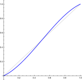
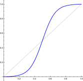
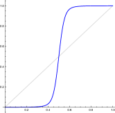
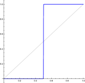
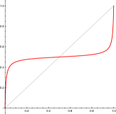
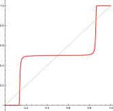
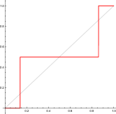
For the function illustrated in Figure 3, 0 and 1 are attractive fixed points and is a non-attractive fixed point. For the function illustrated in Figure 4, 0 and 1 are non-attractive fixed points and is an attractive fixed point.
Lemma 2.6.
Let be an achievable polynomial corresponding to a tree with at least one AND or OR operation. Then
-
1.
The function has an attractive fixed point at 0, a non-attractive fixed point at 1, and no fixed points in if and only if there is a path from the root to a leaf in in which each node represents an AND operation.
-
2.
The function has an non-attractive fixed point at 0, an attractive fixed point at 1, and no fixed points in if and only if there is a path from the root to a leaf in in which each node represents an OR operation.
-
3.
The function has attractive fixed points at 0 and 1, and precisely one non-attractive fixed point in if and only if there is no path from the root to a leaf in in which each node represents an AND operation and there is no path from the root to a leaf in in which each node represents an OR operation. Moreover, is irrational.
[Moore and Shannon, 1956] prove a stronger version of (3). They show that any polynomial corresponding to an arbitrary circuit of AND and OR operations can have at most one fixed point on . We present a similar version of their argument for the setting when is corresponds to a tree.
Proof.
It suffices to prove necessity for each statement.
(1) Let be the polynomials computed by the nodes of some AND path. Since each corresponds to a tree with an AND root, where is the polynomial corresponding to the subtree of the node that does not intersect that AND path. Thus, . For ,
Therefore, has no fixed points on . To see that is an attractive fixed point, note that for any , Thus, . Similarly, is a non-attractive fixed point because for all .
(2) Follows from (1) and Lemma 2.3.
(3) First we show that if the tree has no path of OR operations, then the corresponding polynomial will not have a linear term by proving the contrapositive. The root of a tree corresponding to a polynomial with a linear term must be an OR operation since if the root were an AND operation, the corresponding polynomial would the product of two non-zero polynomials with no constant terms. Given that the root has a linear term and computes for some achievable polynomials and , it follows that or has a linear term. We iteratively apply this argument for the appropriate subtrees and conclude that there is a path of OR operations.
Since has no linear term, for small , . Therefore, there is an neighborhood around zero such that . It follows that , so is an attractive fixed point. The fact that 1 is also an attractive fixed point follows from Lemma 2.3. Since there is no AND path for , there is no OR path in the complementary tree. Thus, 0 is an attractive fixed point of , so 1 is an attractive fixed point of .
Next, we show that there exists some fixed point of on . Since and are attractive fixed points, there exists such that and . By the intermediate value theorem, must cross the line . Thus, there exists some such that .
To prove that is a non-attractive fixed point and that is the unique fixed point on , it suffices to show that for any fixed point , . We use an argument inspired by [Moore and Shannon, 1956] to prove for . Proceed by induction on the size of the tree. Clearly, the statement holds for the leaves which compute the polynomial . Let be the polynomials associated to the two subtrees joined at the root of . If the root is an AND operation, , and we have
The final inequality uses the fact that since , . If the root is an OR operation, and we have
Finally, we prove that is irrational. Suppose for contradiction that where and are relatively prime. Let be the degree of . We may write
where and . Let be the coefficient of the term in . Since is achievable, by Lemma 2.1, each , , and is or . We show by induction that for all for some . First note that . Since , where . Similarly, , so for some . We have , so for some . Assume that for all . We have
Since and are integer multiples of , it follows that is integer. Since is integer, for some . We have shown that are integer multiples of . We have Since is a non-zero integer multiple of , it follows that is not -1 or 1, a contradiction.
Finally, we make some observations about the polynomials associated with the specific family of trees we use in many of our constructions.
Definition 2.7.
Let be a tree on leaves that computes . Let be a tree on leaves that computes .
Lemma 2.8.
Let and be the polynomials corresponding to and respectively. Then has a unique fixed point in the interval and has a fixed point in the interval .
The proof of Lemma 2.8 will use the following elementary inequality.
Lemma 2.9.
For , and any integer , .
of Lemma 2.8..
Lemma 2.10.
Let and where is the polynomial corresponding to . Let be the fixed point of in . Then for all .
Proof.
By definition
Since and are fixed points of , and divide . Therefore, we may write polynomial. We claim that all coefficients of are positive. Note that
Observe
Note that , so for all . Next observe that since comparing the coefficients of the terms on both sides gives . It follows that . For all , Therefore for all .
Since all coefficients of are positive, all derivatives are increasing. In particular the first derivative of is increasing on the interval . Therefore for all .
Lemma 2.11.
Let and be the polynomials corresponding to and respectively. For , there exists some and such that has fixed point . Moreover, . Similarly, for , there exists some and such that has fixed point . Moreover, .
Proof.
3 Convergence of iterative trees to threshold functions
In the previous section, we showed that if the width of each level is infinite, then items at level of an iterative tree evaluate to 1 with probability when each input is independently set to 1 with probability . In this section, we demonstrate ways of selecting so that converges to a -threshold function.
By an abuse of notation, we say that converges to a -threshold function if
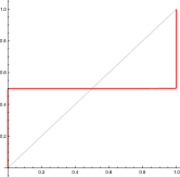
Moreover, we say that converges quadratically to a -threshold function if the corresponding iterative construction exhibits quadratic convergence. The function depicted in Figure 3 converges to a -threshold function.
We now prove that the construction described in Theorem 1.3 converges to a -threshold function.
of Theorem 1.3..
Let be the polynomial that describes the iterative construction in which and are selected with probability and respectively. Since, and ,
Since , the fixed points of are and . We claim that exhibits linear convergence to a -threshold function.
Let be the probability that an input item fires. It suffices to consider the case when . By Corollary 2.4, convergence to 1 for follows from the complementary construction.
First we show that the probability an item at level fires is less than . By definition . Observe that for
It follows that for all either or
For .
Next, we show that at additional levels, the probability an items fires is less than . For ,
It follows
Thus, for , . We have shown that when the input items fire with probability , items level will evaluate to with probability less than .
3.1 Quadratic convergence from iterative trees with small building blocks
In this section we show that using trees with four or five leaves as building blocks, we can construct an iterative tree that converges quadratically to a -threshold function for restricted values of . We begin with a lemma that provides sufficient conditions for quadratic convergence.
Lemma 3.1.
Let be a function corresponding to an iterative construction on inputs that satisfies the following conditions:
-
•
On the interval , has precisely three fixed points: and .
-
•
(Linear Divergence) There exists constants satisfying and and constants such that
-
1.
for , and
-
2.
for .
-
1.
-
•
(Quadratic Convergence) For the constants as above, there exists constants such that and and
-
1.
for , and
-
2.
for .
-
1.
Then exhibits quadratic convergence to a -threshold function, meaning items at level of the corresponding infinite width iterative construction compute a -threshold function with probability at least .
Proof.
Let be the probability an input item fires. First we consider the case when . By the linear divergence assumption, for . It follows that or
Thus for , . Therefore, level items fire with probability at most . Next we show that given a level in which items fire with probability at most , the items at levels higher in the iterative tree fire with probability at most . Let be the probability an item fires at the first level for which the probability an item fires is below . By the quadratic convergence assumption, for . It follows that for , . We have shown that in expectation items at fire with probability less than when . A similar argument applies for .
Remark 3.2.
Let be a function corresponding to an iterative construction with fixed point . Then there exists and for which the quadratic convergence condition of Lemma 3.1 holds if and only if and .
Proof.
Quadratic convergence to is observed if and only if there exists some positive constant sufficiently close to for which all , . Writing according to its Taylor series expansion about implies that such behavior occurs if and only if . Similarly, the observing the Taylor series expansion about allows us to conclude that quadratic convergence to is observed if and only if .
Next, we prove that the construction given in Theorem 1.5A converges quadratically to a - threshold function.
of Theorem 1.5A..
Since , and the probability distribution is well-defined. By construction, and , so
We apply Lemma 3.1. First note that and are fixed points. Let be the fraction of input items firing. It suffices to show convergence to 0 when . By Corollary 2.4, convergence to 1 for follows from the complementary construction.
First we show linear divergence from . Let . We claim for . If , then . If , then . Observe that for any constant and
Thus satisfies the first linear divergence condition.
Next, we show quadratic convergence. Let . Observe that
Since , taking satisfies the first condition of quadratic convergence. Thus, we may apply Lemma 3.1 to conclude that items at level in the limit of the iterative construction compute a -threshold function with probability at least .
It remains to show that no construction using trees with four leaves will yield quadratic convergence to a -threshold function for outside the range . A -threshold function with quadratic convergence must satisfy the following five constraints: (i) , (ii) , (iii) , (iv) , (v) . Solving these equations gives the function
Suppose that can realized by a convex combination of degree four polynomials. Then the leading coefficient of must be between and since all achievable polynomials have leading coefficient or . Thus, , which implies that .
of Theorem 1.5B..
By construction and , so
We apply Lemma 3.1. First note that and are fixed points. Let be the fraction of input items firing. It show convergence to 0 when . By Corollary 2.4, convergence to 1 for follows from the complementary construction.
First we show linear divergence from . Let . We claim that for . If , then . If , then . Thus as in the proof of part A, satisfies the first linear divergence condition. Next we show quadratic convergence. Let . Note that
Since , taking satisfies the first condition of quadratic convergence. Thus, we may apply Lemma 3.1 to conclude that in expectation items at level of the iterative construction compute a -threshold function with probability at least .
It remains to show that no construction using trees with five leaves will yield quadratic convergence to a -threshold function for outside the range . A -threshold function with quadratic convergence must satisfy the following five constraints: (i) , (ii) , (iii) , (iv) , (v) . Such a function will have the form:
Since each achievable polynomial has leading coefficient or , if can written as a convex combination of achievable polynomials of degree five, then
where and are convex combinations of achievable polynomials of degree five with leading coefficient and respectively and . Thus, it suffices to determine the values of for which is achievable through convex combinations and the values of for which is achievable through convex combinations.
Claim: Let . If the function is achievable through convex combinations then , meaning .
Notice that achievable polynomials of degree five with leading coefficient have coefficient (see Table 1). It follows that
so . Next, note that the coefficient of must be non-negative (see Table 1). It follows that
so .
Claim: Let and . If the function is achievable through convex combinations, then and , meaning
Assume is achievable through convex combinations. Notice that for degree five achievable polynomials with and , . It follows that
so and .
Now consider or . By the above claims, and are not achievable through convex combinations. It follows that is not achievable through convex combinations, meaning no construction on trees with five leaves that converges quadratically to a -threshold function for or .
Using a similar technique as in the proof above, it is possible to show that the analogous constructions on six and seven leaves yield iterative constructions that converge quadratically to threshold functions for thresholds in the ranges and respectively. However, it is not possible to generalize such a construction beyond this point. Instead, we observe the emergence of a staircase functions, which will be discussed in Example 4.4.
3.2 Quadratic convergence for arbitrary thresholds.
In this section we show that as approaches 0 or 1, increasingly large building blocks trees are needed to construct an iterative tree that converges quadratically to a - threshold function. Further, we give a construction that exhibits quadratic convergence for arbitrary thresholds near and . We begin by proving Theorem 1.6, which can be restated as follows: Let be an achievable polynomial with fixed points , , and that exhibits quadratic convergence to a -threshold function. Then, has degree at least where .
of Theorem 1.6..
Let be an achievable polynomial with fixed points , , and that exhibits quadratic convergence. Then for sufficiently small, , which implies . For , we have
Since is a fixed point of , . Thus, . It follows that . By Lemma 2.3, if there exists an achievable polynomial with fixed point , then there also exists a complementary achievable polynomial with fixed point . Thus, .
We now prove that a nearly matching iterative construction exists.
To achieve quadratic convergence to thresholds near 0 or 1, we average trees of the form and or and respectively.
of Theorem 1.7..
By Corollary 2.4, it suffices to prove the theorem for . The complement of a construction that achieves quadratic convergence to a -threshold function yields quadratic convergence for to a -threshold function. By Lemma 2.11, there exists and such that has fixed point . Moreover, .
We apply Lemma 3.1 to prove that converges to a -threshold function. Let be the probability an input item is on. First suppose that . We show linear divergence away from . For any constant , and by Lemma 2.11 we have
Thus, is a valid choice for in Lemma 3.1.
Next, we claim that is a valid starting point for quadratic convergence towards 0. We write where . Let . Note that is increasing on the interval since each increases on this interval. For ,
It follows that . Thus, is increasing on the interval . Thus, is a valid choice for in Lemma 3.1.
4 Convergence of iterative constructions to staircase functions
In this section, we explore the possible functions that can be achieved by sampling from the high-level items of iterative constructions with no restrictions on the size of building block trees.
Definition 4.1.
The function is a staircase function if on the interval where , .
We will show in Theorem 4.10 that any staircase function in which each step intersects the line , or more precisely for all , can be approximated by a high-level of an iterative tree.
This result may seem to suggest that the high-level items of these constructions are pseudorandom. However, this is not the case. The output of a high-level item is highly influenced by which of tree it is the root of. The distribution of items firing at a given high-level behaves according to the staircase function, rather than each item individually behaving according to the staircase function.
We begin by giving a couple of examples of staircase functions arising from probability distributions of small trees. The first example is a one step staircase.
Example 4.2.
Consider the iterative construction that selects a tree that computes with probability and a tree that computes with probability . Let be the corresponding polynomial. For , converges to an one step staircase function, i.e. takes value on . For and inputs in which the fraction of inputs firing is not 0 or 1, approximately half the high-level items will fire. Figure 4 illustrates for .
Lemma 4.3.
Consider the iterative construction that selects a tree that computes with probability and a tree that computes with probability where . Let be the corresponding polynomial. Then is the only fixed point of on and it is an attractive fixed point.
Proof.
The only fixed points of are the roots of , which are . To prove that is an attractive fixed point, we show that . We compute . For , we have
We remark that roughly levels are needed (and suffice) to get within of where is the distance of the input from . We omit the proof, which is similar to other proofs of finite bounds in this paper.
In the above construction, a randomly sampled high-level item fires with probability approximately half. However, whether a fixed high-level item fires is not pseudorandom. Given that half of the items at level fire, an item at level that is the root of an building block tree fires with probability . An item at level that is the root of a building block tree fires with probability .
Another simple example of a staircase function is the generalization of the construction given in Theorem 1.5.
Example 4.4.
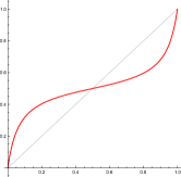
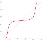
For , the function converges to a three step staircase function. The function has a non-attractive fixed point , a non-attractive fixed point , and an attractive fixed point at . Figure 5 illustrates . Therefore, for inputs in the interval , approximately half the high-level items return and half return . For inputs in the intervals and , high-level items return and respectively with high probability.
Lemma 4.5.
Let . Consider an iterative construction in which and are each selected with probability . Let be the corresponding polynomial. Then is an attractive fixed point of .
Proof.
Let . It suffices to show for . We compute . It follows for that
Finally, we show that it is possible to approximate any staircase function. The proof will rely on Lemma 4.6 and Lemma 4.7, which describe the scope of achievable polynomials for a single tree.
Lemma 4.6.
Let be a fixed point of some achievable polynomial with attractive fixed points and , . Then, for any there exists an achievable polynomial such that for and for
Proof.
First we claim that if is achievable, then is also achievable. Let be the polynomial corresponding to a tree . Define to be the tree modified so that each of the leaves is replaced with a copy of . Let be the tree modified so that each of the leaves is replaced with a copy of . Note that is the polynomial for .
Let be the polynomial for which is a fixed point. It suffices to show that there exists some such that for and for Since is the only fixed point and 0 is an attractive fixed point, for , . Let . Then for all , or . Let . Then for , . A similar argument proves the case when .
The following lemma says that with a single tree, the set of achievable fixed points is dense in . A weaker version of this lemma in which the building blocks of the constructions are arbitrary circuits rather than trees is given by [Moore and Shannon, 1956]. Our proof is inspired by their argument.
Lemma 4.7.
The set of fixed points of achievable polynomials is dense in .
The proof will rely on the following claims.
Claim 4.8.
Let be achievable polynomials such that and has fixed point , . Let . Then for all sufficiently small , there exists such that the fixed point of is in .
Proof.
Note that for any , . Therefore, to prove that there is a fixed point in , it suffices to show that . Since is increasing, for some . By the same arguement in the second paragraph of the proof of Lemma 4.6, there exists such that for any . Taking , we have .
Claim 4.9.
Let be the tree that computes and let be the corresponding polynomial. Then
-
1.
For all and fixed , there exists such that .
-
2.
For all and , .
-
3.
For , is decreasing on .
Proof.
Statement (1) follows from the limit computation
For (2) we first observe that for ,
where denotes the derivative with respect to . For ,
Finally, for (3), note that for .
of Lemma 4.7.
. To prove that the set of achievable fixed points is dense in , it suffices to show that for all , there exists a set of achievable fixed points such that for all , there exists such that . Corollary 2.4 will imply density in .
We construct as follows. Let . Recall has fixed point . Let where is chosen according to Claim 4.9.1 so that . We define and inductively, where is an achievable polynomial with fixed point . Let . By Claim 4.8, there exists such that the fixed point of is less than . Define and to be the corresponding fixed point. Apply Claim 4.9, we observe
It follows that satisfy the desired property that every point in is within of some .
Theorem 4.10.
For any , , such that for all , there exists a probability distribution on a set of trees such that for the corresponding polynomial has the property that for all .
Proof.
We define a probability distribution of a set of trees, the existence of which are guaranteed by Lemma 4.7 and Lemma 4.6. For , let be an achievable fixed point in . Let be an achievable function with fixed point the property that for and for . It follows that for and for . Let and for . Let .
We show is the desired function by computing for . Note that for and for . Observe
Thus, for all .
Theorem 4.10 implies that any staircase function for which for all , can be approximated by the distribution of items at a high-level of an iterative tree. The condition that for all guarantees the heights of each step are fixed points, and therefore the stairs are maintained when is iterated.
5 Finite iterative constructions of threshold trees
In the above section, we analyzed the behavior of iterative trees in the limit with respect to level width. We assumed that for any input the number of items turned on at level of the tree is equal to its expectation, where is the width of level and is the fraction of the inputs turned on. In a “bottom up” construction in which the items of one level are fixed before the next level is built, we note that the chance that the number of items that fire at a given level deviates from expectation is non-trivial. In this section, we give a bound on the width of the levels required to achieve a desired degree of accuracy for finite realizations of iterative constructions.
Remark 5.1.
We can use a transition matrix to directly compute the probability that a high-level item of an iterative construction fires given the width of the levels. Let be the function corresponding to the construction, be the fraction of input items firing, and the width of the levels. Define , , and
for . Then the probability that an item at level fires is .
We will use the following concentration inequalities.
Lemma 5.2.
(Chernoff) Let be independent with and . Then, for any ,
Lemma 5.3.
Let be a sum of binomial random variables with mean . Then, for ,
where
For ease of notation, all statements in this section about the probability of taking some values refers to the probability of taking some values given .
The following lemma describes linear divergence for finite width constructions.
Lemma 5.4.
Consider the construction of a -threshold function in which each level has items and the fraction of input items firing is at least below the threshold . Let be the minimum value of on the interval . Then, with probability at least , the fraction of inputs firing at level will be less than any fixed constant when
where is the linear divergence constant.
Proof.
Let be the fraction of items firing at level . Then . In expectation, the sequence converges to . We will show that with probability at least , the sequence obeys the half-progress relation and therefore for .
Write where is a polynomial in . Let be the minimum value obtained by on the interval . First we compute probability that given by applying Lemma 5.2. Observe
Let and . Then for ,
Next we compute the probability that is the first value for which the half-progress relation is not satisfied given . If the half-progress relation is satisfied meaning , then where . It follows that if the half-progress relation is satisfied for all , then . Thus,
By linear divergence, there exists such that if the sequence satisfies the half-progress relation for all , then . We bound the probability that this does not happen. Let . For ease of notation, let . Observe
Theorem 5.5.
Consider the construction of a -threshold function with linear convergence given in Theorem 1.3 in which each level has items and the fraction of input items firing is at least from the threshold . Then, with probability at least , items at level will accurately compute the threshold function for
Proof.
Let be the fraction of items firing at level . Then . By Corollary 2.4, it suffices to consider the case when the fraction of inputs firing is less that . As proved in Theorem 1.3, in expectation, the sequence convergences to . We will show that with probability at least , the sequence drops below . First we apply Lemma 5.4. Recall that the polynomial corresponding to this construction is and therefore in the statement of Lemma 5.4 is . Let be a constant , and . Thus, with probability at least .
Next we show that given the probability that the sequence continues to obey the half-progress relation (as defined in Lemma 5.4) and drops below is at least . Let . Given a fixed value ,
We compute the probability that is the first value for which the half-progress relation is not satisfied given . If and the half-progress relation is satisfied at then where . It follows that if the half-progress relation is satisfied for all , then . Let . If for all , the half-progress relation is satisfied then . We bound the probability that this does not happen. Let . For ease of notation, let . Observe
Therefore, with probability at least , items at level of an iterative construction with width fire with probability at most for Thus, the iterative construction accurately computes the threshold function with probability at least .
We give a tighter bound for the accuracy of the finite width construction for functions with quadratic convergence. We now prove Theorem 1.8, which can be restated as follows: in order to accurately compute, with probability at least , a -threshold function for inputs in which the fraction of inputs firing is within of , the width of the levels must be
of Theorem 1.8..
Let be the fraction of items firing at level . Then . By Corollary 2.4, it suffices to consider the case when the fraction of inputs firing is less that . As proved in Lemma 3.1, in expectation, the sequence convergences to . We will show that with probability at least , the sequence reaches .
First we apply Lemma 5.4. Recall from the proof of Theorem 1.5, that the minimum value of is on the interval . Therefore for such constructions in the statement of Lemma 5.4 is . For constructions described in Theorem 1.7, the minimum value of is on the interval , as proved in Lemma 2.11. Therefore for such constructions in the statement of Lemma 5.4 is . Let be the constant in quadratic convergence as in Lemma 3.1, and . Thus, with probability at least .
Next, we bound the probability given , that . We say that regresses if . For and as in Lemma 3.1, we apply Lemma 5.3 and obtain
It follows that
Next we bound the probability that given , .
Therefore
Let . It follows and therefore . We now compute
We have shown that given , . Therefore, with probability at least , items at level do not fire for
5.1 Exponential and wild constructions
In this section, we analyze exponential constructions, where items are chosen with probabilities proportional to their weights, and the latter decay exponentially with time, by a factor of . The wild construction is the special case of the exponential construction in which the , i.e. the weights of the items do not decay with time. Here we analyze the wild and exponential constructions for the probability distribution given in Theorem 1.3, which converges linearly to a threshold function. Analogous results, up to constants, hold for the constructions with quadratic convergence.
Throughout this section, we use the following notation. We define to be the probability an item chosen according to the weights at the beginning of the iteration is 1. We define
Additionally, we use the following concentration inequality.
Lemma 5.6.
(Hoeffding) Let be independent random variables with , and . Then for ,
The following two lemmas lay the foundation for the proofs of Theorem 1.9 and 1.10, which prove convergence for the wild and exponential constructions respectively.
Lemma 5.7.
Consider an exponential construction corresponding to a -threshold function given in Theorem 1.3. Let be the probability an item chosen according to the weights at the beginning of the iteration is 1, and let . Let be the event that . Then
where .
Proof.
Note
We now bound Let be random variables where takes value if the item fires. Let . We compute
The statement is equivalent to the following statements, with :
Note that We have
Note that . Applying Hoeffding, we obtain
It follows that
Lemma 5.8.
Consider an exponential construction corresponding to a -threshold function given in Theorem 1.3. Let be the probability an item chosen according to the weights at the beginning of the iteration is 1, and let . Assume for all . Then
Proof.
For , we use the definition of to compute
We compute
We are now ready to prove Theorem 1.9 and Theorem 1.10 which describe the number of items needed to guarantee high accuracy in the wild and exponential constructions respectively.
of Theorem 1.9..
Assume that initial fraction of inputs firing is below the target threshold. The other case follows similarly. We divide the analysis into phases in each of which the total number of items double; in phase , new items are created. Let be the fraction of the first items and the inputs that fire. First we show that with high probability, holds for the entire phase, meaning for all . We call this event where denotes the phase. Lemma 5.7 for states
We bound the probability that does not occur for some phase
Next, we compute the expected progress of the sequence of corresponding to the final items in each phase. Setting , Lemma 5.8 states
We now show that with high probability, the actual progress made by each phase is close to its expectation. Let be indicator random variables where if the item fires, and let . We apply the Hoeffding bound and obtain
Let be the event that . Thus,
We have shown, with probability at least , the events and hold until the fraction of items firing is less that . At this point, an item does not fire and therefore correctly computes the threshold function with probability .
To bound the total number of items, we compute the number of phases needed to achieve We divide the analysis into two parts, when and . In the first part, grows by a constant factor in each phase, while in the second part decays by a constant factor in each phase. So the total number of phases needed is . The total number of items therefore is for some absolute constant .
of Theorem 1.10..
As before, we assume without loss of generality that the initial fraction of inputs firing is below the threshold. We divide the analysis into phases where is the number of items created in a phase, is the number of items created prior to the start of the phase, and is the number of inputs. Let be the probability an item selected according to the probability distribution in the iteration fires. We will set the length of a phase .
First we compute the probability that, holds for the entire phase, meaning for all . We call this event where denotes the phase. Recall the definition of given in Lemma 5.7. For and , we have
where the final inequality follows from the observations that if then , and if , then . Note that , so . Lemma 5.7 implies that
Therefore
Next, we compute the probability that the progress made in a phase is close to its expectation. We ignore the progress made in the first phases. Let be the event that where , , and , given and . First note that
Lemma 5.8 implies that
For phases, we have and therefore,
We now show that with high probability, the actual progress made by each phase is close to its expectation. Let be indicator random variables where if the item fires, and let . Note
We apply the Hoeffding bound, noting that , and obtain
The third step uses the fact that .
Next we compute the total number of phases needed before given holds for all phases and assuming holds after the first phases. For each phase after the first phases, we have
We use the observation that if , then . Observe that
Thus, after phases, the current is less than . Similarly we compute
and conclude that after an additional phases the current is less than . We may assume . The following is an upper bound on the total number of phases needed to have a failure probability less than :
It suffices to show that the probability holds for the first phases is at least and the probability holds for the latter phases is at least . We show in two parts. First we analyze the probability of some event in the for the first phases. We have
For ease of notation, let . For , . For , note . We rewrite the above expression.
Observe
Next we compute
Statement follows from the calculation:
We have shown after phases the next item will fire with probability less than . Since each phase has new items, the total new items created to achieve this is
Finally, we note the lemmas and theorems in this section hold up to modification of constants for wild and exponential constructions corresponding to constructions given in Theorem 1.5 and Theorem 1.7, which exhibit quadratic convergence in the iterative tree setting. However, unlike in the leveled iterative construction, in the exponential and wild constructions we do not see asymptotically faster convergence than the corresponding linear constructions, even in the quadratic regime. In our analysis of the latter constructions, we track the probability that the sequence of goes to zero faster than iterating on curve that is a weighted average of and the function . Regardless of whether has quadratic behavior, has a linear term, implying exhibits linear convergence. Since this yardstick function exhibits linear convergence, this analysis will not yield asymptotically improved results for functions with quadratic convergence.
6 Learning
So far we have studied the realizability of thresholds via neurally plausible simple iterative constructions. These constructions were based on prior knowledge of the target threshold. Here we study the learnability of thresholds from examples. It is important that the learning algorithm should be neurally plausible and not overly specialized to the learning task. We believe the simple results presented here are suggestive of considerably richer possibilities.
We begin with a one-shot learning algorithm. We show that given a single example of a string with , we can build an iterative tree that computes a -threshold function with high probability. Let and be the building block trees in the construction given in Theorem 1.3. The simple LearnThreshold algorithm, described below, has the guarantee stated in Theorem 1.11, which follows from Theorem 1.3.
LearnThreshold():
Input: Levels parameter , a string such that , width parameter .
Output: A finite realization of iterative tree with width .
For each level from to , apply the following iteration times:
(level consists of the input items )
1.
Pick a random input item .
2.
If then let , else let .
3.
Pick items from the previous level.
4.
Build with these items as leaves.
7 Discussion
We have seen that very simple, distributed algorithms requiring minimal global coordination and control can lead to stable and efficient constructions of important classes of functions. Our work raises several interesting questions.
-
1.
What are the ways in which threshold functions are applied in cognition? Object recognition is one application of threshold functions in cognition. For instance, suppose we have items representing features such as “trunk,” “grey,” “wrinkled skin,” and “big ears,” and an item representing our concept of an “elephant.” If a certain threshold of items representing the features we associate with an elephant fire, then the “elephant” item will fire. This structure lends itself to a hierarchical organization of concepts that is consistent with the fact that as we learn, we build on our existing set of knowledge. For example, when a toddler learns to identify an elephant, he does not need to re-learn how to identify an ear. The item representing “ear” already exists and will fire as a result of some threshold function created when the toddler learned to identify ears. Now the item representing “ear” may be used as an input as the toddler learns to identify elephants and other animals.
-
2.
What is an interesting model and neurally plausible algorithm for learning threshold functions of relevant input items? In this scenario, the input is a set of sparse binary strings of length representing examples in which at least of relevant items are firing. The output is an iterative tree that computes a -threshold function on the relevant items. We can formulate the previously described example of learning to identify an elephant as an instance of this problem. Each time the toddler sees an example of an elephant, many features associated with elephant will fire in addition to some features that are not associated with elephants. There may also be features associated with an elephant that are not present in the example and therefore not firing. A learning algorithm must rely on information about the items that are currently firing to learn both the set of relevant items and a threshold function on this set of items. It might also be beneficial to utilize prediction, as e.g., done by Papadimitriou and Vempala [2015a].
-
3.
To what extent can general linear threshold functions with general weights be constructed/learned by cortical algorithms?
- 4.
-
5.
A simple way to include non monotone Boolean functions with the same constructions as we study here, would be to have input items together with their negations (as in e.g., [Savicky, 1990]). What functions can be realized this way, using a distribution on a small set of fixed-size trees?
References
- Arriaga and Vempala [2006] Rosa I. Arriaga and Santosh Vempala. An algorithmic theory of learning: Robust concepts and random projection. Machine Learning, 63(2):161–182, 2006. doi: 10.1007/s10994-006-6265-7. URL http://dx.doi.org/10.1007/s10994-006-6265-7.
- Arriaga et al. [2015] Rosa I. Arriaga, David Rutter, Maya Cakmak, and Santosh S. Vempala. Visual categorization with random projection. Neural Computation, 27(10):2132–2147, 2015. doi: 10.1162/NECO_a_00769. URL http://dx.doi.org/10.1162/NECO_a_00769.
- Boppana [1985] Ravi B. Boppana. Amplification of probabilistic boolean formulas. In Foundations of Computer Science, 1985., 26th Annual Symposium on, pages 20–29, Oct 1985. doi: 10.1109/SFCS.1985.5.
- Brodsky and Pippenger [2005] Alex Brodsky and Nicholas Pippenger. The boolean functions computed by random boolean formulas or how to grow the right function. Random Structures & Algorithms, 27(4):490–519, 2005. ISSN 1098-2418. doi: 10.1002/rsa.20095. URL http://dx.doi.org/10.1002/rsa.20095.
- Dubiner and Zwick [1992] M. Dubiner and U. Zwick. Amplification and percolation [probabilistic boolean functions]. In Foundations of Computer Science, 1992. Proceedings., 33rd Annual Symposium on, pages 258–267, Oct 1992. doi: 10.1109/SFCS.1992.267766.
- Feldman and Valiant [2009] Vitaly Feldman and Leslie G. Valiant. Experience-induced neural circuits that achieve high capacity. Neural Computation, 21(10):2715–2754, 2009. doi: 10.1162/neco.2009.08-08-851.
- Fournier et al. [2009] Hervé Fournier, Danièle Gardy, and Antoine Genitrini. Balanced and/or trees and linear threshold functions. In Proceedings of the Meeting on Analytic Algorithmics and Combinatorics, ANALCO ’09, pages 51–57, Philadelphia, PA, USA, 2009. Society for Industrial and Applied Mathematics. URL http://dl.acm.org/citation.cfm?id=2791158.2791166.
- Friedman [1986] Joel Friedman. Constructing size monotone formulae for the threshold function of boolean variables. SIAM Journal on Computing, 15(3):641–654, 1986.
- Goldman et al. [1993] Sally A Goldman, Michael J Kearns, and Robert E Schapire. Exact identification of read-once formulas using fixed points of amplification functions. SIAM Journal on Computing, 22(4):705–726, 1993.
- Hoory et al. [2006] Shlomo Hoory, Avner Magen, and Toniann Pitassi. Monotone circuits for the majority function. In Approximation, Randomization, and Combinatorial Optimization. Algorithms and Techniques, pages 410–425. Springer, 2006.
- Luby et al. [1998] Michael Luby, Michael Mitzenmacher, and Mohammad Amin Shokrollahi. Analysis of random processes via and-or tree evaluation. In SODA, volume 98, pages 364–373, 1998.
- Moore and Shannon [1956] Edward F Moore and Claude E Shannon. Reliable circuits using less reliable relays. Journal of the Franklin Institute, 262(3):191–208, 1956.
- Papadimitriou and Vempala [2015a] Christos H. Papadimitriou and Santosh S. Vempala. Cortical learning via prediction. In Proc. of COLT, 2015a.
- Papadimitriou and Vempala [2015b] Christos H. Papadimitriou and Santosh S. Vempala. Cortical computation. In Proc. of PODC, 2015b.
- Rosch [1978] E. Rosch. Principles of categorization. In Eleanor Rosch and Barbara Lloyd, editors, Cognition and Categorization. Lawrence Elbaum Associates, 1978.
- Rosch et al. [1976] Eleanor Rosch, Carolyn B. Mervis, Wayne D. Gray, David M. Johnson, and Penny Boyes-braem. Basic objects in natural categories. COGNITIVE PSYCHOLOGY, 8:382–439, 1976.
- Savicky [1987] Petr Savicky. Boolean functions represented by random formulas. Commentationes Mathematicae Universitatis Carolinae, 28(2):397–398, 1987.
- Savicky [1990] Petr Savicky. Random boolean formulas representing any boolean function with asymptotically equal probability. Discrete Mathematics, 83(1):95 – 103, 1990. ISSN 0012-365X. doi: http://dx.doi.org/10.1016/0012-365X(90)90223-5. URL http://www.sciencedirect.com/science/article/pii/0012365X90902235.
- Servedio [2004] Rocco A. Servedio. Monotone boolean formulas can approximate monotone linear threshold functions. Discrete Applied Mathematics, 142(1–3):181 – 187, 2004. ISSN 0166-218X. doi: http://dx.doi.org/10.1016/j.dam.2004.02.003. URL http://www.sciencedirect.com/science/article/pii/S0166218X04000174. Boolean and Pseudo-Boolean Functions.
- Valiant [1984] Leslie G. Valiant. Short monotone formulae for the majority function. Journal of Algorithms, 5(3), 1984.
- Valiant [1994] Leslie G. Valiant. Circuits of the mind. Oxford University Press, 1994. ISBN 978-0-19-508926-4.
- Valiant [2000] Leslie G. Valiant. A neuroidal architecture for cognitive computation. J. ACM, 47(5):854–882, 2000. doi: 10.1145/355483.355486.
- Valiant [2005] Leslie G. Valiant. Memorization and association on a realistic neural model. Neural Computation, 17(3):527–555, 2005. doi: 10.1162/0899766053019890.
8 Appendix
| Degree | Polynomials in |
|---|---|
| 1 | (0,1) |
| 2 | (0, 0, 1) |
| (0, 2, -1) | |
| 3 | (0, 0, 0, 1) |
| (0, 1, 1, -1) | |
| (0, 0, 2, -1) | |
| (0, 3, -3, 1)) | |
| 4 | ((0, 0, 0, 0, 1) |
| (0, 1, 0, 1, -1) | |
| (0, 0, 1, 1, -1) | |
| (0, 2, 0, -2, 1) | |
| (0, 0, 0, 2, -1) | |
| (0, 1, 2, -3, 1) | |
| (0, 0, 3, -3, 1) | |
| (0, 4, -6, 4, -1) | |
| (0, 0, 2, 0, -1) | |
| (0, 0, 4, -4, 1)) |
| Degree | Polynomials in |
|---|---|
| 5 | (0, 0, 0, 0, 0, 1) |
| (0, 1, 0, 0, 1, -1) | |
| (0, 0, 1, 0, 1, -1) | |
| (0, 2, -1, 1, -2, 1) | |
| (0, 0, 0, 1, 1, -1) | |
| (0, 1, 1, 0, -2, 1) | |
| (0, 0, 2, 0, -2, 1) | |
| (0, 3, -2, -2, 3, -1) | |
| (0, 0, 0, 0, 2, -1) | |
| (0, 1, 0, 2, -3, 1) | |
| (0, 0, 1, 2, -3, 1) | |
| (0, 2, 1, -5, 4, -1) | |
| (0, 0, 0, 3, -3, 1) | |
| (0, 1, 3, -6, 4, -1) | |
| (0, 0, 4, -6, 4, -1) | |
| (0, 5, -10, 10, -5, 1) | |
| (0, 0, 0, 2, 0, -1) | |
| (0, 1, 2, -2, -1, 1) | |
| (0, 0, 0, 4, -4, 1) | |
| (0, 1, 4, -8, 5, -1) | |
| (0, 0, 1, 1, 0, -1) | |
| (0, 0, 3, -1, -2, 1) | |
| (0, 0, 2, 1, -3, 1) | |
| (0, 0, 6, -9, 5, -1) |