On short-term traffic flow forecasting
and its reliability

Abstract

Recent advances in time series, where deterministic and stochastic modelings as well as the storage and analysis of big data are useless, permit a new approach to short-term traffic flow forecasting and to its reliability, i.e., to the traffic volatility. Several convincing computer simulations, which utilize concrete data, are presented and discussed.

1 Introduction

We recently proposed a new feedback control law for ramp metering (Abouaïssa, Fliess, Iordanova & Join (2012)), which is based on the most fruitful model-free control setting (Fliess & Join (2013)). It has not only been patented but also successfully tested in 2015 on a highway in northern France. It will soon be implemented on a larger scale. We are therefore lead to study another important topic for intelligent transportation systems, i.e., short-term traffic flow forecasting: it plays a key rôle in the planning and development of traffic management. This importance explains the extensive literature on this subject since at least thirty years. Several surveys (see, e.g., Bolshinsky & Friedman (2012); Chang, Zhang, Yao & Yue (2011); Lippi, Bertini & Frasconi (2013); Smith, Williams & Oswald (2002); Vlahogianni, Karlaftis & Golias (2014)) provide useful informations on the various approaches which have been already employed: regression analysis, time series, expert systems, artificial neural networks, fuzzy logic, etc. We follow here another road, i.e., a new approach to time series (Fliess & Join (2009, 2015a, 2015b); Fliess, Join & Hatt (2011a, b)):

• A quite recent theorem due to Cartier & Perrin (1995) yields the most important notions of trends and quick fluctuations, which do not seem to have any analogue in other theoretical approaches. Among those existing approaches, the dominant one today has been developed for econometric goals (see, e.g., Mélard (2008), Tsay (2010), and Meuriot (2012) for some historical and epistemological issues). It is quite popular in traffic flow forecasting.

• Although its origin lies in financial engineering, it has been recently applied for short-term meteorological forecasts for the purpose of renewable energy management (Join, Voyant, Fliess, Nivet, Muselli, Paoli & Chaxel (2014); Voyant, Join, Fliess, Nivet, Muselli & Paoli (2015); Join, Fliess, Voyant & Chaxel (2016)).

• Like in model-free control (Fliess & Join (2013)), no deterministic or probabilistic mathematical modeling is needed. Moreover the storage and analysis of big data is useless.Those facts open new perspectives to intelligent knowledge-based systems.

The reliability of those computations should nevertheless be examined, at least for a better risk understanding. This subject, which is crucial for any type of approach, has been much less studied (see, e.g., Guo, Huang & Williams (2014); Laflamme & Ossenbruggen (2014); Zhang, Zhang & Haghani (2014), and the references therein). This risk may of course be studied via the concept of volatility, which may be found everywhere in finance (see, e.g., Tsay (2010); Wilmott (2006)). The strong attacks against the very concept of volatility seem to have been ignored in the community studying intelligent transportation systems. We are thus reproducing the following quote from Fliess, Join & Hatt (2011a). Wilmott (2006) (chap. 49, p. 813) writes: Quite frankly, we do not know what volatility currently is, never mind what it may be in the future. The lack moreover of any precise mathematical definition leads to multiple ways for computing volatility which are by no means equivalent and might even be sometimes misleading (see, e.g., Goldstein & Taleb (2007)). Our theoretical formalism and the corresponding computer simulations will confirm what most practitioners already know. It is well expressed by Gunn (2009) (p. 49): Volatility is not only referring to something that fluctuates sharply up and down but is also referring to something that moves sharply in a sustained direction. Let us stress that in econometrics and in financial engineering the notion of volatility is usually examined via the returns of financial assets. This setting seems to be pointless in the context of traffic flow. Defining the volatility directly from the time series (see also Fliess, Join & Hatt (2011b)) makes much more sense.

Our viewpoint on time series is sketched in Section 2. Section 3 investigates the fundamental notion of persistence. The forecasting techniques for the traffic flow on a French highway and the corresponding computer experiments are discussed in Section 4. Short concluding remarks may be found in Section 5.

2 Revisiting time series

2.1 Time series via nonstandard analysis

Take the time interval $[0,1]\subset\mathbb{R}$ and introduce as often in nonstandard analysis (see, e.g., (Lobry & Sari (2008); Fliess & Join (2009, 2015a)), and some of the references therein, for basics in nonstandard analysis) for the infinitesimal sampling

$${\mathfrak{T}}=\{0=t_{0}<t_{1}<\dots<t_{\nu}=1\}$$

where $t_{i+1}-t_{i}$, $0\leq i<\nu$, is infinitesimal, i.e., “very small”. A time series $X(t)$ is a function $X:{\mathfrak{T}}\rightarrow\mathbb{R}$.

A time series ${\mathcal{X}}:{\mathfrak{T}}\rightarrow\mathbb{R}$ is said to be quickly fluctuating, or oscillating, if, and only if, the integral $\int_{A}{\mathcal{X}}dm$ is infinitesimal, i.e., very small, for any appreciable interval, i.e., an interval which is neither very small nor very large.

According to a theorem due to Cartier & Perrin (1995) the following additive decomposition holds for any time series $X$, which satisfies a weak integrability condition,

$$\boxed{X(t)=E(X)(t)+X_{\tiny{\rm fluctuation}}(t)}$$ (1)

where

• the mean, or average, $E(X)(t)$ is “quite smooth.”,

• $X_{\tiny{\rm fluctuation}}(t)$ is quickly fluctuating.

The decomposition (1) is unique up to an infinitesimal.

2.2 On the numerical differentiation of a noisy signal

Let us start with the first degree polynomial time function $p_{1}(\tau)=a_{0}+a_{1}\tau$, $\tau\geq 0$, $a_{0},a_{1}\in\mathbb{R}$. Rewrite thanks to classic operational calculus with respect to the variable $\tau$ (see, e.g., Yosida (1984)) $p_{1}$ as $P_{1}=\frac{a_{0}}{s}+\frac{a_{1}}{s^{2}}$. Multiply both sides by $s^{2}$:

$$s^{2}P_{1}=a_{0}s+a_{1}$$ (2)

Take the derivative of both sides with respect to $s$, which corresponds in the time domain to the multiplication by $-t$:

$$s^{2}\frac{dP_{1}}{ds}+2sP_{1}=a_{0}$$ (3)

The coefficients $a_{0},a_{1}$ are obtained via the triangular system of equations (2)-(3). We get rid of the time derivatives, i.e., of $sP_{1}$, $s^{2}P_{1}$, and $s^{2}\frac{dP_{1}}{ds}$, by multiplying both sides of Equations (2)-(3) by $s^{-n}$, $n\geq 2$. The corresponding iterated time integrals are low pass filters which attenuate the corrupting noises (see Fliess (2006) for an explanation). A quite short time window is sufficient for obtaining accurate values of $a_{0}$, $a_{1}$. Note that estimating $a_{0}$ yields the trend.

The extension to polynomial functions of higher degree is straightforward. For derivative estimates up to some finite order of a given smooth function $f:[0,+\infty)\to\mathbb{R}$, take a suitable truncated Taylor expansion around a given time instant $t_{0}$, and apply the previous computations. Resetting and utilizing sliding time windows permit to estimate derivatives of various orders at any sampled time instant.

Remark 1

See (Fliess, Join & Sira-Ramírez (2008); Mboup, Join & Fliess (2009); Sira-Ramírez, García-Rodríguez, Cortès-Romero & Luviano-Juárez (2014)) for more details.

2.3 Forecasting

Set the following forecast $X_{\text{est}}(t+\Delta T)$, where $\Delta T>0$ is not too “large”,

$$X_{\text{forecast}}(t+\Delta T)=E(X)(t)+\left[\frac{dE(X)(t)}{dt}\right]_{e}\Delta T$$ (4)

where $E(X)(t)$ and $\left[\frac{dE(X)(t)}{dt}\right]_{e}$ are estimated like $a_{0}$ and $a_{1}$ in Section 2.2. Let us stress that what we predict is the trend and not the quick fluctuations (see also Fliess & Join (2009); Fliess, Join & Hatt (2011b); Join, Voyant, Fliess, Nivet, Muselli, Paoli & Chaxel (2014); Voyant, Join, Fliess, Nivet, Muselli & Paoli (2015)).

2.4 Volatility

Contrarily to our previous approach via returns (Fliess, Join & Hatt (2011a, b)), we use here the difference $X(t)-E(X)(t)$ between the time series and its trend. If this difference is square integrable, i.e., if $(X(t)-E(X)(t))^{2}$ is integrable, volatility is defined via the following standard deviation type formula:

$${{\text{\bf vol}}}(X)(t) = \sqrt{E\left(X-E(X)\right)^{2}}$$

$$\simeq \sqrt{E(X^{2})-E(X)^{2}}$$

3 Persistence

3.1 Definition

The persistence method is the simplest way of producing a forecast. It assumes that the conditions at the time of the forecast will not change, i.e.,

$$X_{\text{forecast}}(t+\Delta T)=X(t)$$ (5)

3.2 Scaled Persistence

Scaled persistence, which is often encountered in meteorology (see, e.g., (Lauret, Voyant, Soubdhari, David & Poggi (2015)), and (Join, Voyant, Fliess, Nivet, Muselli, Paoli & Chaxel (2014); Voyant, Join, Fliess, Nivet, Muselli & Paoli (2015))) improves Formula (5) by writing

$$X_{\text{Pe}}(t+\Delta T)=E(X)(t)\times S_{c}(t)$$ (6)

where

• $E(X)(t)$ is estimated like $a_{0}$ in Section 2.1,

• the scaling factor $S_{c}(t)$ will be made precise according to the situation,

• contrarily to (5) quick fluctuations are disregarded and the trend is emphasized.

4 Case study

4.1 Description

Consider a section of the highway A25 from Dunkirk (Dunkerque in French) to Lille (see Figure 1). There are two lanes on this section, and about $900$m between two measurements stations. Congestions often occur.

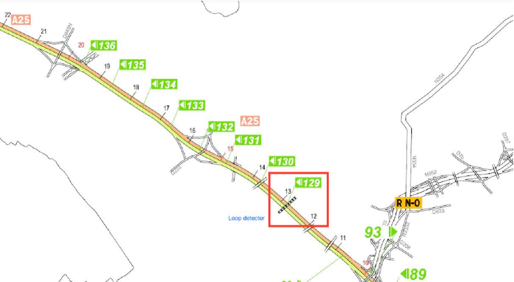
Figure 1: Our highway section

The traffic volume, the occupation rate and and the mean vehicle speed, which yield excellent traffic characterizations, are measured. We focus here on the traffic volume $Q(t)$, in veh/min. It is registered every minute from 1 to 30 June 2014, and displayed in Figure 2-(a). Two single days are detailed in Figures 2-(b) and 2-(c). In all those Figures the trend is also drawn. It is computed by using 100 points and the following non-causal moving average

$$\text{mean}(Q(t-49),...,Q(t+50))=\frac{Q(t-49)+\dots+Q(t+50)}{100}$$ (7)

4.2 Forecastings

Let us emphasize that forecasting errors will be defined with respect to the trend derived from (7). Three forecast horizons are considered$:$ $5$, $15$, and $60$ minutes. Set $X(t)=Q(t)$. The term $E(Q)(t)$ in (4) and (6) are deduced from the causal moving average

$$E_{100}(Q)(t)=\text{mean}(Q(t-99),...,Q(t))=\frac{Q(t-99)+\dots+Q(t)}{100}$$

The scaling factor $S_{c}(t)$ in (6) is given by

$$S_{c}(t)=\frac{E_{100}(Q)(t-1\text{day}+\Delta T)}{E_{100}(Q)(t-1\text{day})}$$

where

• $\text{1day}=60\times 24=1440\ \text{minutes}$,

• $\Delta T$ is equal to one of the three following values$:$ 5, 15, 60 minutes.

Then (4) and (6) become respectively

$$Q_{\text{A}}(t+\Delta T)=E_{100}(Q)(t)+\left[\frac{dE_{100}(Q)(t)}{dt}\right]_{e}\Delta T$$ (8)

and

$$Q_{\text{Pe}}(t+\Delta T)=E_{100}(Q)(t)\times\frac{E_{100}(Q)(t-1\text{day}+\Delta T)}{E_{100}(Q)(t-1\text{day})}$$ (9)

Computer experiments show that (8) and (9) suffer respectively from rather large overshoots and undershoots. In order to remedy this annoying fact write (9) in the form

$$Q_{\text{Pe}}(t+\Delta t)=E_{100}(Q)(t)+E_{100}(Q)(t)\frac{Sc(t)-1}{\Delta t}\Delta t$$

It yields the following forecasting equation

$$Q_{\text{MixedForecast}}(t+\Delta t)=E_{100}(Q)(t)+\tilde{a}_{1}(t)\Delta t$$ (10)

where $\tilde{a}_{1}$ is equal to

1. $\frac{dE_{100}(Q)(t)}{dt}$ if its module is smaller than the module of $E_{100}(Q)(t)\frac{Sc(t)-1}{\Delta t}$,

2. $E_{100}(Q)(t)\frac{Sc(t)-1}{\Delta t}$ if not.

4.3 Computer Experiments

Results are displayed in Figures 3, 4 and 5 . The superiority of the forecasting (10) is obvious. Table 1, with its squared errors, provide a quantified comparison of the various approaches.

Table 1: $\sum\text{Errors}^{2}$

Horizon	Pe	Al [gain in %]	Mi [gain in %]
$t+5\text{min}$	2.08e+06	1.01e+06 [105%]	8.75e+05 [137%]
$t+15\text{min}$	2.64e+06	1.7335e+06 [52%]	1.23e+06 [114%]
$t+60\text{min}$	1.15e+07	8.47e+06 [36%]	4.29e+06 [169%]

4.4 Volatility

Figure 6 displays the various trends, which are computed via the non-causal mean (7), for three time scales: $100$, $250$, or $500$ minutes. Note that larger is the time scale smoother is the trend. On the other hand Figure 7 shows a volatility increase. Due to a lack of space, only forecasting volatility via Formula (8) for a $15$ minutes time horizon is displayed in Figure 8, where the middle value, i.e., $250$ minutes, is utilized for calculating the trend. The results are rather good.

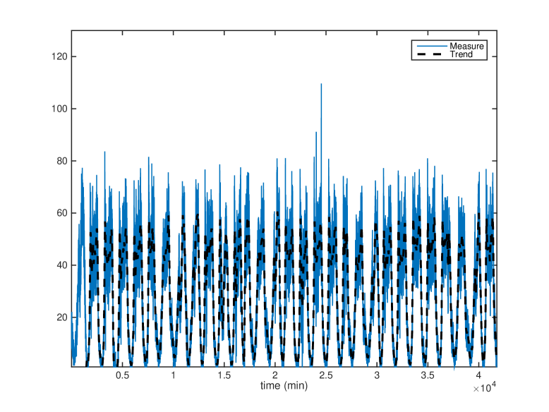
(a) From 1 to 30 June 2014

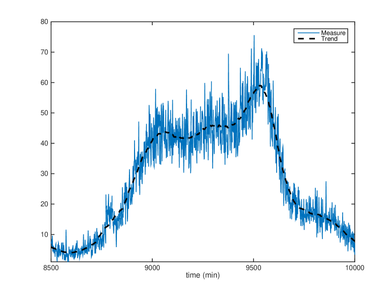
(b) Zoom 1

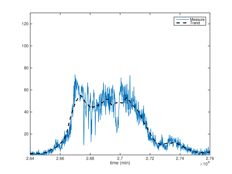
(c) Zoom 2

Figure 2: Measures and trend

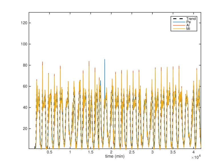
(a) The whole set of data

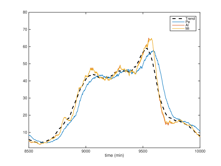
(b) Zoom 1

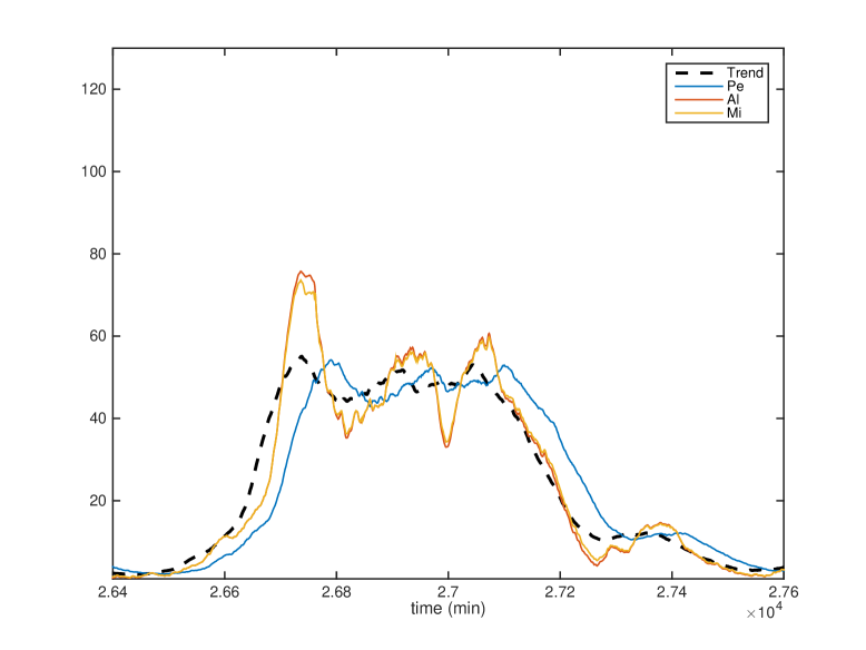
(c) Zoom 2

Figure 3: 5 minutes forecasts

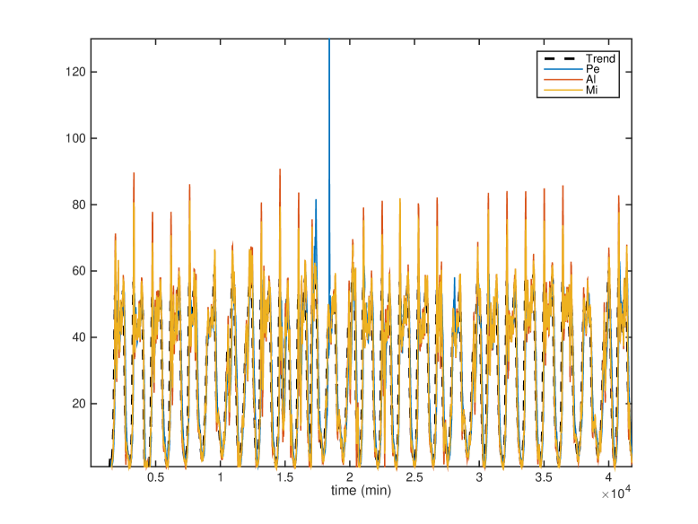
(a) From 1 to 30 June 2014

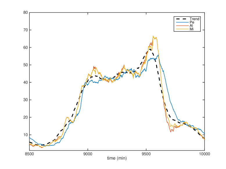
(b) Zoom 1

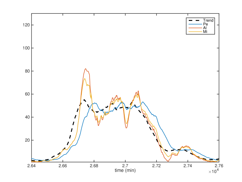
(c) Zoom 2

Figure 4: 15 minutes forecasts

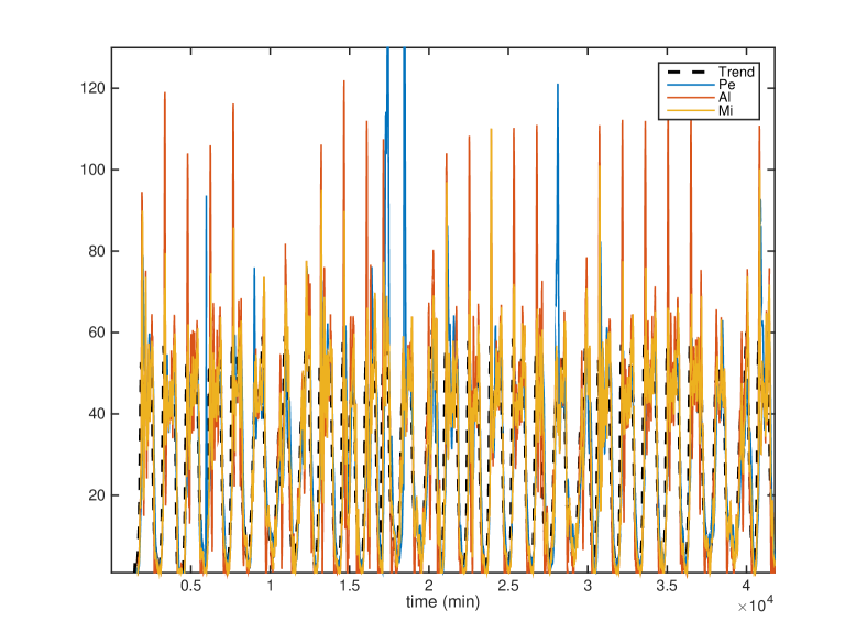
(a) The whole set of data

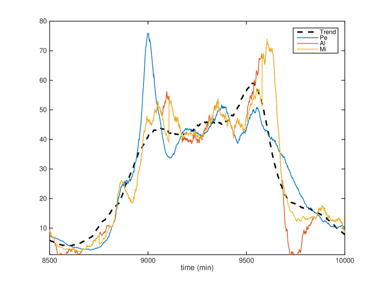
(b) Zoom 1

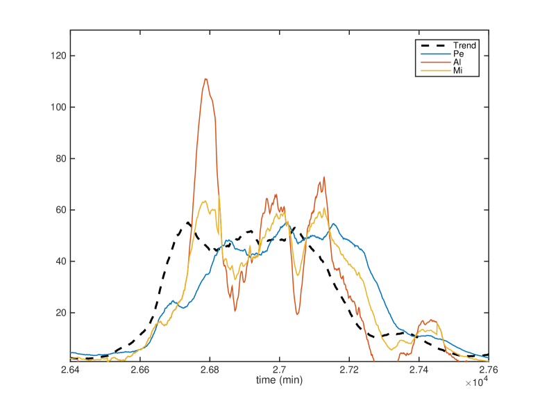
(c) Zoom 2

Figure 5: 60 minutes forecasts

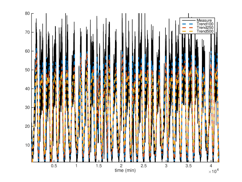
(a) The whole set of data

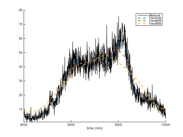
(b) Zoom 1

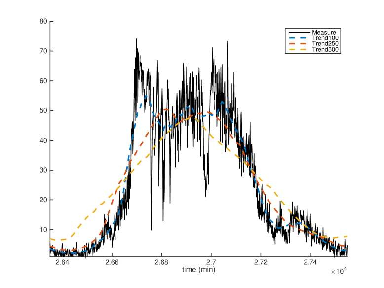
(c) Zoom 2

Figure 6: Trend and time scales

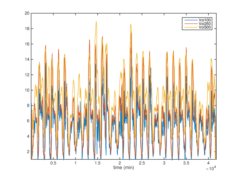
(a) The whole set of data

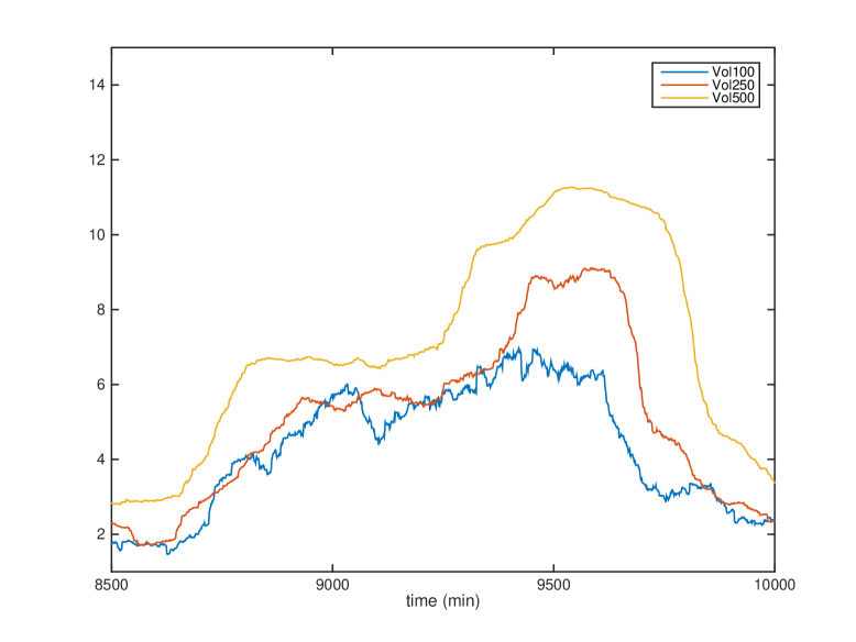
(b) Zoom 1

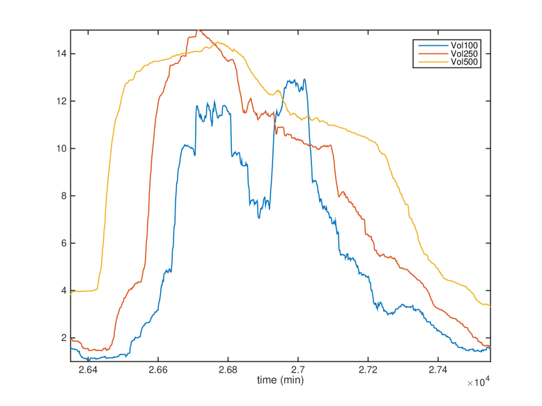
(c) Zoom 2

Figure 7: Volatility and time scales

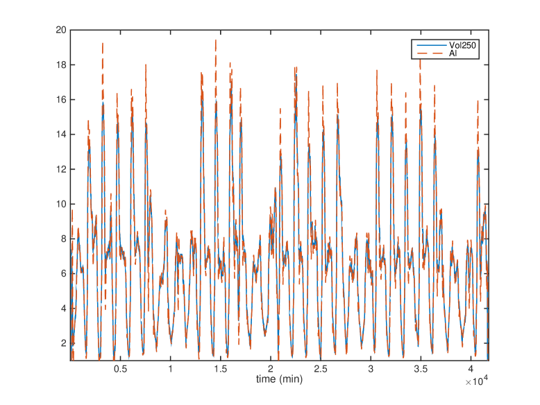
(a) The whole set of data

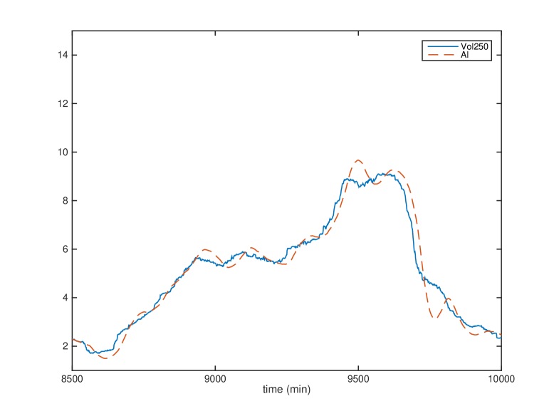
(b) Zoom 1

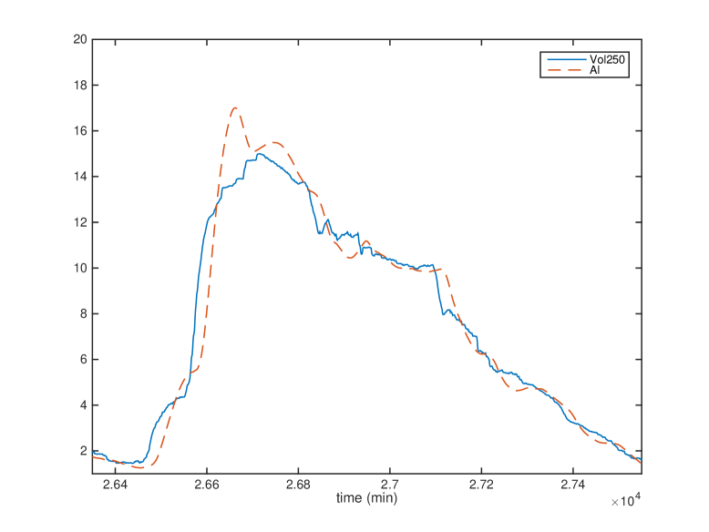
(c) Zoom 2

Figure 8: Forcasting volatility

5 Conclusion

Although encouraging our preliminary results need not only to be further developed but also to be compared with other existing approaches. Let us emphasize that such comparisons began to be discussed for short-term meteorological forecasts by Join, Voyant, Fliess, Nivet, Muselli, Paoli & Chaxel (2014) and Voyant, Join, Fliess, Nivet, Muselli & Paoli (2015). Our methods were easier to implement and much less demanding in terms of historical data. For a deeper study of reliability and risk, see Join, Fliess, Voyant & Chaxel (2016) where the notion of confidence bands may be extended to traffic management in a straightforward way.

The Cerema (Centre d’études et d’expertise sur les risques, l’environnement, la mobilité et l’aménagement) provided the authors with the necessary data for the highway A25. This highway is managed by the DIRN (Direction Interdépartementale des Routes Nord) via the ALLEGRO (Agglomération liLLoise Exploitation Gestion de la ROute) system.

References

- Abouaïssa, Fliess, Iordanova & Join (2012) H. Abouaïssa, M. Fliess, V. Iordanova, C. Join. Freeway ramp metering control made easy and efficient. 13th IFAC Symp. Control Transportation Systems, Sofia, 2012. Online: https://hal.archives-ouvertes.fr/hal-00711847/en/
- Bolshinsky & Friedman (2012) E. Bolshinsky, R. Friedman. Traffic flow forecast survey. Tech. Rep., Comput. Sci. Dept., Technion, Haifa, 2012.
- Cartier & Perrin (1995) P. Cartier, Y. Perrin. Integration over finite sets. F. & M. Diener editors: Nonstandard Analysis in Practice, pp. 195–204, Springer, 1995.
- Chang, Zhang, Yao & Yue (2011) G. Chang, Y. Zhang, D. Yao, Y. Yue. A summary of short-term traffic flow forecasting methods. ICCTP, 2011.
- Fliess (2006) M. Fliess. Analyse non standard du bruit. C.R. Acad. Sci. Paris Ser. I, 342 797–802, 2006
- Fliess & Join (2009) M. Fliess, C. Join. A mathematical proof of the existence of trends in financial time series. In A. El Jai, L. Afifi, E. Zerrik, editors, Systems Theory: Modeling, Analysis and Control, 43–62, Presses Universitaires de Perpignan, 2009. Online: https//hal.archives-ouvertes.fr/inria-00352834/en/
- Fliess & Join (2013) M. Fliess, C. Join. Model-free control. Int. J. Control, 86 2228–2252, 2013.
- Fliess & Join (2015a) M. Fliess, C. Join, Towards a new viewpoint on causality for time series. ESAIM ProcS, 49 37–52, 2015a. Online: https://hal.archives-ouvertes.fr/hal-00991942/en/
-
Fliess & Join (2015b)
M. Fliess, C. Join, Seasonalities and cycles in time series: A fresh look with computer experiments. Paris Finan. Manag. Conf., Paris, 2015b. Online:
https://hal.archives-ouvertes.fr/hal-01208171/en/ - Fliess, Join & Hatt (2011a) M. Fliess, C. Join, F. Hatt. Volatility made observable at last. 3es J. Identif. Modél. Expérim., Douai, 2011a. Online: https//hal.archives-ouvertes.fr/hal-00562488/en/
- Fliess, Join & Hatt (2011b) M. Fliess, C. Join, F. Hatt. A-t-on vraiment besoin d’un modèle probabiliste en ingénierie financière ? Conf. Médit. Ingén. Sûre Syst. Compl., Agadir, 2011b. Online: https//hal.archives-ouvertes.fr/hal-00585152/en/
- Fliess, Join & Sira-Ramírez (2008) M. Fliess, C. Join, H. Sira-Ramírez. Non-linear estimation is easy. Int. J. Modelling Identif. Control, 4 12–27, 2008. Online: https//hal.archives-ouvertes.fr/inria-00158855/en/
- Goldstein & Taleb (2007) D.G. Goldstein, N.N. Taleb. We don’t quite know what we are talking about when we talk about volatility. J. Portfolio Manage., 33: 84–86, 2007.
- Gunn (2009) M. Gunn. Trading Regime Analysis. Wiley, 2009.
- Guo, Huang & Williams (2014) J. Guo, W. Huang, B.M. Williams. Adaptive Kalman filter approach for stochastic short-term traffic flow prediction and uncertainty quantifications. Transport. Res. C, 43 50–64, 2014.
-
Join, Fliess, Voyant & Chaxel (2016)
C. Join, M. Fliess, C. Voyant, F. Chaxel. Solar energy production: Short-term forecasting and risk management. 8th IFAC Conf. Manufact. Model. Manag. Contr., Troyes, 2016.
Online:
https://hal.archives-ouvertes.fr/hal-01272152/en/ -
Join, Voyant, Fliess, Nivet, Muselli, Paoli & Chaxel (2014)
C. Join, C. Voyant, M. Fliess, M. Muselli, M.-L. Nivet, C. Paoli, F. Chaxel. Short-term solar irradiance and irradiation forecasts via different time series techniques: A preliminary study.
3rd Int. Symp. Environ. Friendly Energy Appl., Paris, 2014. Online:
https://hal.archives-ouvertes.fr/hal-01068569/en/ - Laflamme & Ossenbruggen (2014) E.M. Laflamme, P.J. Ossenbruggen. The effect of stochastic volatility in predicting highway breakdowns. Symp. 50 Years Traffic Flow Theory, Portland, 2014.
- Lauret, Voyant, Soubdhari, David & Poggi (2015) P. Lauret, C. Voyant, T. Soubdhan, M. David, P. Poggi. A benchmarking of machine learning techniques for solar radiation forecasting in an insular context. Solar Energ., 112 446–457, 2015.
- Lippi, Bertini & Frasconi (2013) M. Lippi, M. Bertini, P. Frasconi. Short-term traffic flow forecasting: An experimental comparison of time-series analysis and supervised learning. IEEE Trans. Intel. Transport. Syst., 14 871–882, 2013.
- Lobry & Sari (2008) C. Lobry, T. Sari. Nonstandard analysis and representation of reality. Int. J. Control, 81 519–53, 2008.
- Mboup, Join & Fliess (2009) M. Mboup, C. Join, M. Fliess. Numerical differentiation with annihilators in noisy environment. Num. Algo., 50 439–467, 2009.
- Mélard (2008) G. Mélard. Méthodes de prévision à court terme. Ellipses & Presses Universitaires de Bruxelles, 2008.
- Meuriot (2012) V. Meuriot. Une histoire des concepts des séries temporelles. Harmattan–Academia, 2012.
- Sira-Ramírez, García-Rodríguez, Cortès-Romero & Luviano-Juárez (2014) H. Sira-Ramírez, C. García-Rodríguez, J. Cortès-Romero, A. Luviano-Juárez, Algebraic Identification and Estimation Methods in Feedback Control Systems. Wiley, 2014.
- Smith, Williams & Oswald (2002) B.L. Smith, B.M. Williams, R.K. Oswald. Comparison of parametric and nonparametric models for traffic flow forecasting. Transport. Res. C, 10 303–321, 2002.
- Tsay (2010) R.S. Tsay. Analysis of Financial Time Series (3rd ed.). Wiley, 2010.
- Vlahogianni, Karlaftis & Golias (2014) E.I. Vlahogianni, M.G. Karlaftis, J.C. Golias. Short-term traffic forecasting: Where we are and where we are going. Transport. Res. C, 43 3–19, 2014.
-
Voyant, Join, Fliess, Nivet, Muselli & Paoli (2015)
C. Voyant, C. Join, M. Fliess, M.-L. Nivet, M. Muselli, & C. Paoli. On meteorological forecasts for energy management and large historical data: A first look.
Renew. Ener. Power Quality J., 13, 2015. Online:
https//hal.archives-ouvertes.fr/hal-01093635/en/ - Wilmott (2006) P. Wilmott. Paul Wilmott on Quantitative Finance, 3 vol. (2nd ed.). Wiley, 2006.
- Yosida (1984) K. Yosida. Operational Calculus (translated from the Japanese). Springer, 1984.
- Zhang, Zhang & Haghani (2014) Y. Zhang, Y. Zhang, A, Haghani. A hybrid short-term traffic flow forecasting method based on spectral analysis and statistical volatility model. Transport. Res. C, 43 65–78, 2014.