Influence of stability islands in the recurrence of particles in a static oval billiard with holes

Abstract

Statistical properties for the recurrence of particles in an oval billiard with a hole in the boundary are discussed. The hole is allowed to move in the boundary under two different types of motion: (i) counterclockwise periodic circulation with a fixed step length and; (ii) random movement around the boundary. After injecting an ensemble of particles through the hole we show that the surviving probability of the particles without recurring - without escaping - from the billiard is described by an exponential law and that the slope of the decay is proportional to the relative size of the hole. Since the phase space of the system exhibits islands of stability we show that there are preferred regions of escaping in the polar angle, hence given a partial answer to an open problem: Where to place a hole in order to maximize or minimize a suitable defined measure of escaping.

I Introduction

A billiard is a dynamical system where a point-like particle moves with constant speed along straight lines confined to a piecewise and smooth boundary to where it experiences specular reflections Ref1 . In such type of collisions the tangent component of the velocity of the particle, measured with respect to the border where collision happened, is unchanged while the normal component reverses sign. Originally, the investigation on billiards was introduced in the seminal paper of Birkhoff Ref2 in the beginning of last century – therefore introducing a new research area – and since from there the scientific research on this topic has experienced a great development. Indeed, Birkhoff considered the investigation of the motion of a free point-like particle in a bounded manifold. Modern investigations on billiards however are connected with the results of Sinai Ref3 and Bunimovich Ref4 ; Ref5 who made rigorous demonstrations in the subject. The billiards theory has also been used in many different kinds of physical systems, including experiments on superconductivity Ref6 , wave guides Ref7 , microwave billiards Ref8 ; Ref9 , confinement of electrons in semiconductors by electric potentials Ref10 ; Ref12 , quantum tunneling Ref11 and many others.

The dynamics of a particle in a billiard can be matched into one of the following three possibilities: (i) regular; (ii) ergodic and; (iii) mix. The circular billiard is a typical example of case (i) since it is integrable thanks to the conservation of energy and angular momentum Ref1 . The elliptic billiard is also integrable and observables preserved are the energy and angular momenta about the two foci Ref13 . Case (ii) corresponds to systems containing zero measure stable periodic orbits, hence dominated by chaotic dynamics as the Bunimovich stadium Ref4 ; Ref14 as well as the Sinai billiard Ref3 . Finally the case (iii) includes billiards where the phase space has mixed dynamics therefore containing either regular dynamics characterized by periodic islands and/or invariant spanning curves and chaos as for instance, the annular billiard Ref11 . In Ref. Ref13 , Sir Michael Berry discussed a family of billiards of the oval-like shapes. The radius in polar coordinates has a control parameter, ($\epsilon$), which leads to a smooth transition from a circumference with ($\epsilon=0$) – hence integrable – to a deformed form with $(\epsilon\neq 0)$. For sufficiently small ($\epsilon$), a special set of invariant spanning curves exists in the phase space corresponding to the so called whispering gallery orbits. They are orbits moving around the billiard, close to the border, with either positive (counterclockwise dynamics) or negative (clockwise dynamics) angular momentum. As soon as the parameter reaches a critical value Ref15 , the invariant spanning curves are destroyed as well as the whispering gallery orbits.

Billiards can also be considered in the context of recurrence of particles Ref16 ; Ref17 , particularly related to the Poincaré recurrence Ref16 ; Ref18 . The recurrence can be measured from the injection and hence from the escape of an ensemble of particles by a hole made in the boundary. The dynamics is made such that a particle injected through the hole is allowed to move inside the billiard suffering specular reflections with the boundary until it encounters the hole again. At this point the particle escapes from the billiard. The number of collisions that the particle has had till the escape is computed and another particle with different initial condition is introduced in the system. The dynamics is repeated until a large ensemble of particles is exhausted. The statistics of the recurrence time is then obtained. The known results are that for a totally chaotic dynamics, the survival probability – probability that the particle survives without escaping through the hole – is described by an exponential function Ref19 . When there are resonance islands, or Kolmogorov-Arnold-Moser (KAM) curves, to where the particles can be sticky around for long times, the dynamics is then changed to a slower decay conjectured in Ref. Ref18 to be described by a power law of universal scaling with an exponent from the order of $-2.57$. Therefore, as considered recently in a chapter book by Dettmann Ref19 who discusses some open problems in billiard with holes, a particular question was posed regarding to escape of particles: Optimisation: Specify where to place a hole to maximize or minimize a suitable defined measure of escaping.

In the current paper we discuss the recurrence of particles in an oval-like shaped billiard with a hole in the boundary and our main goal is to move a step further as an attempt to give a partial answer to the above question. The hole is allowed to move around the boundary under two different rules: (i) periodic and; (ii) randomly. In either cases, we define fixed places around the boundary to where the hole can be introduced. In the case (i) the hole moves counterclockwise under two circumstances. As soon as the particle is injected through the hole, its position moves if the particle escapes through it with less than $5$ collisions with the boundary. If the particles does not escape until $5$ collisions, it moves counterclockwise to a neighboring allowed position and wait until a escape or to more than other $5$ collisions. The billiard perimeter is divided in 63 equally steps for the hole tour. This process repeats injecting and escaping particles until all the ensemble is exhausted. In the case (ii) the hole moves randomly around the boundary respecting the time of $5$ collisions. The survival probability, obtained from the recurrence time that the particle spent to escape, is accounted for a large ensemble of noninteracting particles. At each time of a escape, the polar angle and the angle of the trajectory particle are known, hence the corresponding position in the phase space where the escape happened is known as well. Then a statistics of the density of particles that escaped from a given region of the phase space can be computed. We show that the density of escape measured in both polar angle as well as the angle of the particle’s trajectory present peaks and valleys. The peaks are associated to the high density occupation in the phase space while the valleys are mostly linked to the periodic islands domain. Our results then give a partial answer to the above open question, at least for the oval billiard which has mixed phase space.

This paper is organized as follows. In Sec. II we discuss the model and the equations that fully describe the dynamics of the system. The escape properties for the particles when the hole moves periodically around the boundary are made in Sec. III. The survival probability for the particles when the hole moves randomly around the boundary is discussed in Sec. IV while our final remarks and conclusions are drawn in Sec. V.

II The static oval billiard

We discuss in this section how to obtain the equations that fully describe the dynamics of the system. To start with, the radius of the boundary in polar coordinate is given by

$$R(\theta,\epsilon,p)=1+\epsilon\cos(p\theta),$$ (1)

where $\theta$ is the polar coordinate, $\epsilon$ corresponds to a perturbation parameter of the circle and $p>0$ is an integer number. For $\epsilon=0$ the system is integrable. The phase space is foliated Ref1 and only periodic and quasi-periodic orbits are observed. For $\epsilon\neq 0$ the phase space is mixed containing both periodic, quasi-periodic and chaotic dynamics. When $\epsilon$ reaches the critical value Ref15 $\epsilon_{c}={1/(1+p^{2})}$ the invariant spanning curves, corresponding to the whispering gallery orbits are destroyed and only chaos and periodic islands are observed. This happens when the boundary is concave for $\epsilon<\epsilon_{c}$ and is not observed for $\epsilon>\epsilon_{c}$ when the boundary exhibits segments that are convex.

The dynamics is described by a two dimensional nonlinear mapping relating the variables $(\theta_{n},\alpha_{n})\rightarrow(\theta_{n+1},\alpha_{n+1})$ where $\theta$ denotes the polar angle to where the particle collides and $\alpha$ represents the angle that the trajectory of the particles does with a tangent line at the collision point. Fig. 1 illustrates the representation of the angles.

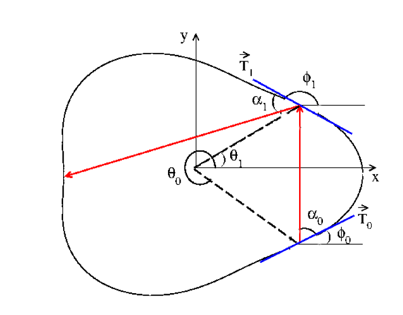
Figure 1: (Color online). Illustration of the angles involved in the billiard.

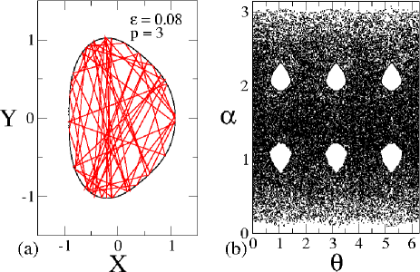
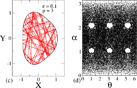
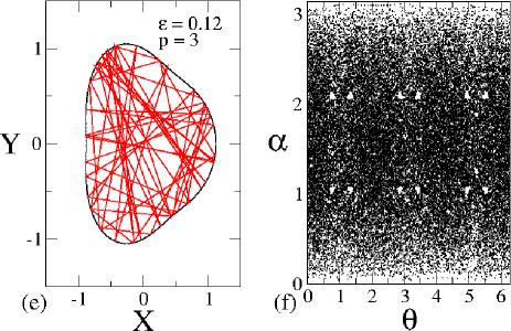
Figure 2: (Color online). Plot of the geometry shapes (a,c,e) and chaotic dynamics in such a boundaries in (b,d,f). The parameters used were $p=3$ and (a,b) $\epsilon=0.08<\epsilon_{c}$, (c,d) $\epsilon=0.1=\epsilon_{c}$ and (e,f) $\epsilon=0.12>\epsilon_{c}$.

For an initial condition $(\theta_{n},\alpha_{n})$ the position of the particle is written as $X(\theta_{n})=[1+\epsilon\cos(p\theta_{n})]\cos(\theta_{n})$ and $Y(\theta_{n})=[1+\epsilon\cos(p\theta_{n})]\sin(\theta_{n})$. The angle of the tangent vector at the polar coordinate $\theta_{n}$ is $\phi_{n}=\arctan\left[{Y^{\prime}(\theta_{n})\over{X^{\prime}(\theta_{n})}}\right]$, where $X^{\prime}(\theta)=dX(\theta)/d\theta$ and $Y^{\prime}(\theta)=dY(\theta)/d\theta$. Since there are no forces acting on the particle from collision to collision, it then moves along a straight line so its trajectory is given by

$$Y(\theta_{n+1})-Y(\theta_{n})=\tan(\alpha_{n}+\phi_{n})[X(\theta_{n+1})-X(\theta_{n})],$$ (2)

where $\theta_{n+1}$ is the the new polar coordinate of the particle when it hits the boundary, which is to be obtained numerically. The angle $\alpha_{n+1}$ given the slope of the trajectory of the particle after a collision is

$$\alpha_{n+1}=\phi_{n+1}-(\alpha_{n}+\phi_{n}).$$ (3)

The mapping is then written in a compact way as

$$\left\{\begin{array}[]{ll}F(\theta_{n+1})&=R(\theta_{n+1})\sin(\theta_{n+1})-Y(\theta_{n})-\tan(\alpha_{n}+\phi_{n}){}\\ &\times[R(\theta_{n+1})\cos(\theta_{n+1})-X(\theta_{n})]{}\\ \alpha_{n+1}&=\phi_{n+1}-(\alpha_{n}+\phi_{n})\end{array}\right.~{}$$ (4)

where $\theta_{n+1}$ is obtained numerically from $F(\theta_{n+1})=0$ with $R(\theta_{n+1},\epsilon,p)=1+\epsilon\cos(p\theta_{n+1})$ and $\phi_{n+1}=\arctan\left[{Y^{\prime}(\theta_{n+1})}/{X^{\prime}(\theta_{n+1})}\right]$.

Figure 2(a,c,e) represent the sketch of the boundary and few collisions of a typical chaotic orbit while Fig. 2(b,d,f) correspond to the chaotic dynamics shown in the phase space. The parameters that we have used were $p=3$ and in Figures (a,b) $\epsilon=0.08<\epsilon_{c}$, in Figures (c,d) $\epsilon=0.1=\epsilon_{c}$ and in Figures (e,f) $\epsilon=0.12>\epsilon_{c}$.

III Statistical properties of the open oval billiard: the periodic case

Let us now discuss some statistical properties for the recurrence of particles considering a hole of size $h$ placed on the boundary which can move regularly along the boundary with counterclockwise circulation. The hole has a constant aperture. Our initial results were obtained for a fixed $h=0.1$. Other values have been used too and the results are similar to the ones presented here. The hole is centered at $\theta_{ct}$ and we allow it to move around the boundary into $63$ possible places. The places are fixed and separated from each other by a step size of length $2\pi/63$. The dynamics of the particle is started from a hole, i.e., it is injected through it. The particle then moves around the boundary according to the equations of the mapping. If it happens that the particle visits the hole again within the interval of less than $5$ collisions, it escapes through the hole, a new and different initial condition is started and the process goes on. However, if the particle does not visit the same hole to where it was injected, the hole closes and opens a step above and has a time-life of $5$ collisions. If the particle does not reach such hole, it closes and reopens a step above with a life-time of $5$ collisions until the particle finds one hole to escape.

The procedure to study the escape of the particles and the survival probability is to inject an ensemble of $10^{6}$ particles from a hole placed in $\theta\in(0,h)$ and evolve the dynamics of each particle at most $10^{6}$ collisions with the boundary. The initial conditions were chosen such that $10^{3}$ of them were uniformly distributed in $\theta_{0}\in(0,h)$ and $10^{3}$ with different $\alpha_{0}\in(0,\pi)$. The statistical analysis were made in terms of the number of collisions of each particle until escape of the billiard. The process is repeated again until the whole ensemble is exhausted. Then a histogram showing the frequency of escapes is constructed. Fig. 3(a) shows a histogram for the frequency of escape $H(n)$ for three different parameters, as labeled in the figure. The horizontal axis represents the number of collisions of the particle before reaching the hole and the vertical axis is the fraction of particles which escaped through a hole.

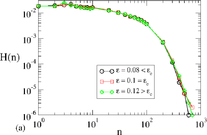
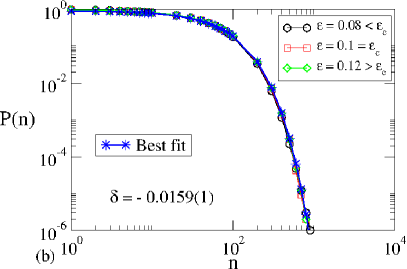
Figure 3: (Color online). (a) Histogram for the escape frequency of particles as a function of the number of collisions; (b) The survival probability of the particles. An exponential fitting furnishes $\delta=-0.0159(1)$. The parameter used was $p=3$ while the values of $\epsilon$ are shown in the plots.

The integration of $H(n)$, gives the distribution of particles that do not escape through the hole until collision $n$. It corresponds to the survival probability and is given by

$$P(n)={1\over{N}}\sum_{n=1}^{N}N_{surv}(n),$$ (5)

where $N$ is the number of initial conditions and $N_{surv}$ is the number of the particles that survived until the $n^{th}$ collision. Fig. 3(b) shows the results for the survival probability obtained for $p=3$ and for an ensemble of $10^{6}$ different particles. As one sees the decay law is exponential. We notice that after about $10^{3}$ collisions almost all initial conditions escaped from the billiard for a hole size $h=0.1$. The decay is fitted by a curve of the type

$$P(n)=P_{0}e^{n\delta},$$ (6)

where $P_{0}$ is a constant, $\delta$ is the slope of the decay and $n$ is the number of collisions. The slope obtained by an exponential fit was $\delta=-0.0159(1)$, which is remarkably close to the relative size of the hole, i.e., the size of the hole over the whole length of the boundary ${h\over{2\pi}}={0,1\over{2\pi}}=0.0159\ldots$.

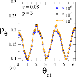
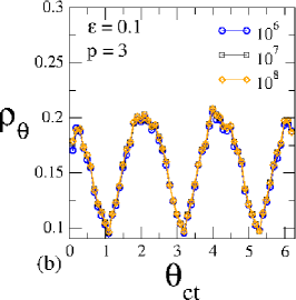
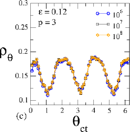
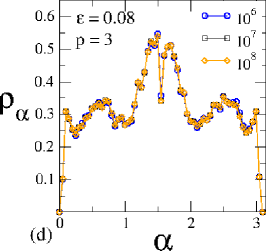
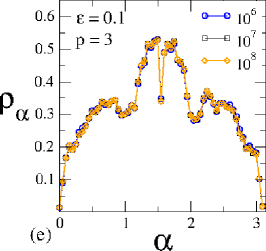
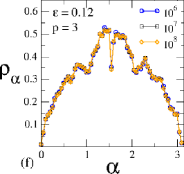
Figure 4: (Color online). Escaping density $\rho_{\theta}~{}vs.~{}\theta$ for the following parameters: (a) $\epsilon=0.08$; (b) $\epsilon=0.1$ and; (c) $\epsilon=0.12$. Three ensemble sizes were used, as labeled in the figures. The density of escaping $\rho_{\alpha}~{}vs.~{}\alpha$ is shown for: (d) $\epsilon=0.08$; (e) $\epsilon=0.1$ and; (f) $\epsilon=0.12$.

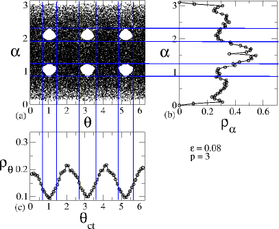
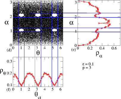
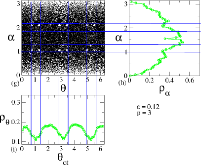
Figure 5: (Color online). Connection of the peaks and valleys with the existence and absence of periodic regions in the phase space. The phase space is shown for: (a) $\epsilon=0.08$; (d) $\epsilon=0.1$ and; (g) $\epsilon=0.12$. The escape density $\rho_{\theta}~{}vs.~{}\theta$ is shown in; (b), (e) and (h) for the same combinations of control parameters. The density $\rho_{\alpha}~{}vs.~{}\alpha$ is presented in: (c), (f), and (i).

Let us now discuss the density of escape measured as a function of the position of the hole $\theta_{ct}$. To do that we consider three different sizes for the ensemble of initial conditions, namely $10^{6}$, $10^{7}$ and $10^{8}$. Fig. 4 shows a plot of density $\rho_{\theta}~{}vs.~{}\theta_{ct}$ for the parameters: (a) $\epsilon=0.08$; (b) $\epsilon=0.1$ and; (c) $\epsilon=0.12$. We see from the figure the existence of peaks and valleys and that none difference of the curves for different ensemble sizes. The peaks correspond to the values of $\theta_{ct}$ to where the escape of particles is most probably to be observed, hence giving a clear evidence of preferable regions of escaping, while the valleys show the lower probability of escaping.

We may think of at first what is the reason that yields the density of escape to be smaller in some regions and larger in others. A possible answer for this could be linked directly to the periodic regions of the phase space. Then it becomes natural to look at the density of escaping also as a function of the variable $\alpha$. Fig. 4 (d-f) show the statistical results for the density of escape $\rho_{\alpha}~{}vs.~{}\alpha$ where $\alpha$ is the last coordinate the particle had prior the escape for the same parameters used in Fig. 4(a-c). We see again that there are preferential regions to escape. Either peaks and valleys are also observed. The peaks and the valleys observed in both figures, must be connected to each other and with the properties of the phase space. Thinking in this way Fig. 5(a-i) show a connection of the valleys with the corresponding periodic regions in the phase space while the peaks are linked to the absence of periodic regions the phase space.

From the analysis of both Figs. 4 and 5 we can give a partial answer to the open question posed in Ref19 . The maximization of escape is provided at a region of the phase space with absence of periodic islands. In the complementary way, the minimization of escape is produced in a region of the phase space filled with islands of periodicity. This then reduces the effective size of the chaotic sea reducing the chances of a particle to escape if a hole is placed in the coordinates of periodic regions.

We must also mention a second and indirect phenomenon which is linked to the regions of periodic islands, particularly small islands and a possible channel among them, and that may lead to an extra life-time for the particles which is a phenomena called as stickiness Ref18 . Although a chaotic orbit can pass very close to a periodic region, in whose domain there exist islands, the dynamics can be trapped locally avoiding visitation to other places in the phase space, hence giving extra life to particles trapped around such regions.

IV Statistical properties of the open oval billiard: the random case

In this section we discuss the results for the hole moving around the boundary but occupying random positions. The rule which controls the hole movement around the boundary is very similar to the previous section. However, instead of sequentially moving a step, the hole moves randomly along the $63$ possible places defined along the boundary. To chose a random position for placing the hole we used the so called RAN2 random number generator Ref22 .

The results obtained for this type of moving hole are remarkably similar to those discussed in the previous section. For a hole size $h=0.1$, the slope of the decay of the survival probability obtained numerically is $\delta=-0.0163(1)$, very comparable to the results obtained in previous section.

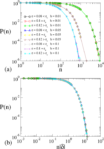
Figure 6: (Color online). (a) Plot of survival probability of the particles obtained for a hole moving randomly around the boundary as a function of $n$ for different hole sizes; (b) Their overlap onto a single and hence universal plot after a transformation $n\rightarrow n|\delta|$.

Let us now discuss the influence of the hole size on the escape of particles. The exponential decay, marking the escaping dynamics of the particles does not change its pattern when the size of the hole is varied, at least for the range of holes considered here. For a smaller hole there is a shift in time allowing to the particles more opportunities to move along the phase space without escaping as compared to a larger hole. Therefore a scaling transformation $n\rightarrow n|\delta|$ rescales all curves obtained for the survival probability considering different values of $h$ onto a single and universal plot, as shown in Fig. 6.

V Discussion and Conclusions

In this paper we studied some statistical properties for the escaping and hence survival of particles inside an oval-like shaped billiard. We introduced a hole that changes its position on the boundary in two different ways: (i) first the hole moves around the boundary in a continuous stepwise either after a escape of a particle or after $5$ collisions with the boundary without finding the hole. In the second case the hole moves randomly after a escape or after a $5$ collisions life-time. For both cases the survival probability decays exponentially and the slope of the decay is proportional to the size of the hole over the total length of the boundary.

We notice there are preferential regions along the phase space to where the escape of particles is facilitated, hence leading to a maximum escape. However, there are also regions in the space of phase, particularly those exhibiting stability islands, that influence quite negatively for the escape.

The discussion presented here allowed us to give a partial answer to the open question posed in Ref19 . We conclude that the maximization of escaping is obtained from a region of the phase space with absence of periodic islands and with higher density of visitation of particles. The opposite is also observed, the minimization of the escape can be produced from a region of the phase space filled with islands of periodicity. Stickiness can also provide with an extra life timefor the particles, by extending their dynamics over the chaotic sea.

VI Acknowledgements

MH thanks to CAPES for the financial support. REC and EDL acknowledge support from the Brazilian agencies FAPESP under the grants 2014/00334-9 and 2012/23688-5 and CNPq through the grants 306034/2015-8 and 303707/2015-1.

References

- (1) C. Nikolai, R. Markarian, Chaotic Billiards, American Mathematical Society, (2006).
- (2) G. Birkhoff, Dynamical Systems, American Mathematical Society, Providence, RI, USA, 1927.
- (3) Ya. G. Sinai, Russian Mathematical Surveys, 25, 137 (1970).
- (4) L. A. Bunimovich, Functional Analysis and Its Applications, 8, 73 (1974).
- (5) L. A. Bunimovich and Ya. G. Sinai, Communications in Mathematical Physics, 78, 479 (1981).
- (6) H. D. Graf et al., Phys. Rev. Lett. 69, 1296 (1992).
- (7) E. Persson et al., Phys. Rev. Lett. 85, 2478 (2000).
- (8) J. Stein, H. J. Stokmann, Phys. Rev. Lett. 68, 2867 (1992).
- (9) H. J. Stokmann, Quanum Chaos: An Introduction (Cambridge University Press), (1999).
- (10) T. Sakamoto et al., Jpn. J. Appl. Phys. 30, L1186 (1992).
- (11) J. P. Bird, J Phys. Condens. Matter. 11, R413 (1992).
- (12) O. Bohigas, D. Boosé, R. Egydio de Carvalho, V. Marvulle, Nuclear Phys. A. 560, 197 (1993).
- (13) M. V. Berry, Eur. J. Phys. 2, 91 (1981).
- (14) L. A. Bunimovich, Funct. Anal. Appl., 8, 254 (1974).
- (15) D. F. M. Oliveira, E. D. Leonel, Commun. Nonlinear Sci. Numer. Simulat., 15, 1092 (2010).
- (16) C. V. Abud, R. Egydio de Carvalho, Phys. Rev. E. 88, 042922 (2013).
- (17) M. F. Demmers, P. Wright, L-S. Young, Commun. Math. Phys., 294, 353388 (2010).
- (18) E. G. Altmann, T. Tél, Phys. Rev. E, 79, 016204 (2009).
- (19) Book chapter: Recent advances in open billiards with some open problems: C. P. Dettmann, in Frontiers in the study of chaotic dynamical systems with open problems, Editted by Z. Elhadj and J. C. Sprott. World Scientific, (2011).
- (20) W. H. Press, B. P. Flannery, S. A. Teukolsky, W. T. Vetterling, Numerical Recipes in Fortran 77: The Art of Scientific Computing, Cambridge University Press, 2 edition, (1992).