The optimal Boson energy for superconductivity in the Holstein model
Abstract
We examine the superconducting solution in the Holstein model, where the conduction electrons couple to the dispersionless Boson fields, using the Migdal-Eliashberg theory and Dynamical Mean Field Theory. Although different in numerical values, both methods imply the existence of an optimal Boson energy for superconductivity at a given electron-Boson coupling. This non-monotonous behavior can be understood as an interplay between the polaron and superconducting physics, as the electron-Boson coupling is the origin of the superconductor, but at the same time traps the conduction electrons making the system more insulating. Our calculation provides a simple explanation on the recent experiment on sulfur hydride, where an optimal pressure for the superconductivity was observed. The validities of both methods are discussed.
pacs:
74.20.-z, 74.20.Fg, 74.25.KcI Introduction
Since the discovery of superconductivity by Onnes Onnes (1911), countless efforts have been dedicated to understanding the microscopic origin of the phenomena, as well as to searching/synthesizing materials of high superconducting critical temperatures (). Based on the microscopic theories, the superconductors are classified as “conventional” and “unconventional” superconductors. The former class can be well described by the BCS (Bardeen-Cooper-Schrieffer) theory Cooper (1956); Bardeen et al. (1957a, b) or its variants Kirzhnits et al. (1973), whereas the latter class is still controversial in its microscopic mechanisms Mann (2011). The unconventional superconductors include the layered materials such as cuprates Bednorz and Müller (1986); Damascelli et al. (2003) and iron-based materials Kamihara et al. (2006, 2008); Ge et al. (2015). The multi-orbital nature and strong electron correlation intrinsically complicate the problem, as there can be several competing phases Dagotto (1994); Imada et al. (1998). For this reason, searches of unconventional high temperature superconductors are mainly based on “perturbing the existing superconductors” (via doping, applying pressure, interfacing with other materials … etc) and “exhausting all possible compounds” Hosono et al. (2015). The searches of conventional high temperature superconductors, on the other hand, are essentially guided by the BCS theory, or by the more realistic Eliashberg model Eliashberg (1960); Migdal (1958); Morel and Anderson (1962); Allen and Dynes (1975); Bergmann and Rainer (1973); Grimvall (1981); Allen and Mitrovic (1983), which is different from BCS theory in its explicit inclusion of the phonon (or the Boson in general) degrees of freedom. In the Eliashberg model, the origin of the effective electron-electron attraction is the electron-phonon coupling, and the main factor against superconductivity, the Coulomb repulsion, is treated at a semi-empirical level by one parameter Morel and Anderson (1962); McMillan (1968); Allen and Mitrovic (1983). Therefore, the key to enhance is to control the phonon-related parameters – the Debye frequency and the electron-phonon coupling. Recent experiments on sulfur hydride, whose motivation behind is to increase the Debye frequency by using light elements (H) and applying high pressure, exhibit a record superconducting at 203 K Drozdov et al. (2015). The strong enhancement of superconducting in the mono-layer FeAs or FeSe on SrTiO3 substrate is deeply related to the interfacial optical phonon mode Qing-Yan et al. (2012); Ge et al. (2015); Lee et al. (2014); Rademaker et al. (2016); Wang et al. (2016). Attempts of using Boson other than phonons, such as the plasma in meta-materials, to mediate the electron-electron attraction also appear promising Smolyaninova et al. (2014); Smolyaninov and Smolyaninova (2015).
The Holstein model Holstein (1959), where the conduction electrons couple to the dispersionless Boson fields, is the simplest model that captures the physics of conventional superconductors. In this work, we examine the superconducting solution in Holstein model, using the Migdal-Eliashberg (ME) theory Migdal (1958); Eliashberg (1960) and the Dynamical Mean Field Theory (DMFT) Georges et al. (1996); Kotliar and Vollhardt (2004); Maier et al. (2005); Gull et al. (2011) with the exact diagonalization (ED) impurity solver. This model has been intensely studied Freericks et al. (1993); Freericks and Jarrell (1994, 1995); Benedetti and Zeyher (1998); Deppeler and Millis (2002); Wellein and Fehske (1997); Kalosakas et al. (1998); Meyer et al. (2002); Werner and Millis (2007); De Filippis et al. (2012); Murakami et al. (2015); Vekić et al. (1992); Sykora et al. (2009), but relatively few explicitly break the gauge symmetry to obtain the superconducting solution Hague (2005); Murakami et al. (2014). Although different in numerical values, both ME and DMFT imply the existence of an optimal Boson energy for superconductivity at a given electron-Boson coupling. The existence of the optimal Boson energy can be expected from the BCS theory – if we take the cutoff energy as the Boson energy , and the effective electron-electron attraction as (an estimate from the second-order perturbation) with being the electron-Boson coupling, the superconducting gap behaves as with the electron density of states at the Fermi energy. The ME theory actually gives a very similar behavior. The DMFT, however, gives different ground state under some parameter regimes, as it captures the polaron effect, where the Boson that mediates the electron-electron attraction can make the system insulating. The DMFT calculation also elucidates the relationship between the polaron solution and the superconducting solution.
The rest of the paper is organized as follows. In Section II we describe the Holstein model and the two methods – the ME theory and DMFT – to obtain the superconducting solutions. We provide a simple picture that is emerged from DMFT, on how the Boson field can lead to the superconducting solution. In Section III, we present our main results, compare them to those in the literature, and discuss their validities and implications. Finally a brief conclusion is given in Section IV.
II Holstein model and solvers
In this section we introduce the Holstein model, and the two solvers we used – the ME theory and DMFT – to solve this model. The expressions of the main observables, including the superconducting gap and the pairing amplitude, are given. Several hints of the existence of the optimal Boson energy for superconductivity will be highlighted.
II.1 Holstein model and superconducting gap
The Holstein model is given by
| (1) |
Here represents the Fermion degree of freedom, whereas represents the Boson degree of freedom. In Eq. (1), we can rewrite and in the real-space coordinate as
| (2) |
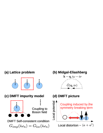
This form is more natural for DMFT calculations. The Holstein model in the real-space representation is illustrated in Fig. 1(a). In this work, we shall consider the conduction band of semicircular density of states (DOS) . This corresponds to the Bethe lattice of infinite dimension, a limit where the DMFT result becomes exact. The bandwidth is fixed at with , and all energy scales, including the electron-Boson coupling and the Boson energy , are measured in . We only show the results at half filling, and the -1 in of Eq. (2) ensures that the Boson field is at its ground state when the local occupation is 1 (half-filled) Werner and Millis (2007).
To obtain the superconducting solutions, both ME theory and DMFT self-consistently determine the Nambu Green’s functions at the Matsubara frequencies. Defining a Nambu spinor as , the lattice Green function (a 22 matrix) on the imaginary-time axis and at the Matsubara frequency is given by
| (3) |
where represents the ground state expectation value. Using Pauli matrices
| (4) |
the self-energies and the lattice Green’s functions are parameterized as
| (5) |
with being the non-interacting Green’s function. Without loss of generality, we can choose , and the task is to determine , , and self-consistently using some approximation.
When the lattice Green’s function are obtained, its poles determine the single-particle excitations. From Eq. (5), the poles are determined by (with the analytical continuation )
| (6) |
For the normal state (), the poles are given by , which are simply the quasi-particle (quasi-hole) excitations. For the non-zero , the excitation occurs at . When neglecting the dependence (an approximation we are using in this paper), the superconducting gap is obtained by energy difference , with . Keeping only the constant term of and , the gap is approximately
| (7) |
where and are used. In addition to the superconducting gap, the superconductivity can also be characterized by the pairing amplitude
| (8) |
Note that is a dimensionless quantity, whose amplitude is always smaller than one. Eq. (7) and Eq. (8) will be used to characterize the superconducting state.
II.2 Migdal-Eliashberg theory
The Migdal-Eliashberg theory is formulated in the momentum space. It keeps only the “Fock” contribution in the self energies [see Fig. 1(b) for the diagrammatic representation]:
| (9) |
is the off-diagonal part of the Green’s function, is the coupling that annihilates an electron of momentum and creates an electron of momentum , and is the Boson Green’s function. Substituting Eq. (9) into Eq. (5), we obtain the equation for , , and as
| (10a) | ||||
| (10b) | ||||
| (10c) | ||||
where . For the Holstein model defined in Eq. (1), we have and . We further simplify the equation by neglecting the momentum dependence, i.e. , , and obtain the coupled equations
| (11) |
with , , and . With the semicircular DOS , and are evaluated by
| (12) |
with . We solve Eq. (11) by iteration. The zero-temperature results obtained by using and keeping 4000 Matsubara frequencies; the results are checked against those obtained using lower temperature and keeping more Matsubara frequencies. Three comments about Eq. (11) are worth noting. First, by linearizing Eq. (11) ( components), det determines the critical temperature . Second, due to the neglect of momentum dependence in the self energy, we expect the superconducting gap obtained using the approximation is under-estimated. Finally, as the magnitudes of are small at both small and large , Eq. (11) suggests a optimal for the superconductivity. At this stage it is simply a mathematical observation, and we shall give a more physical discussion on Section II.D and Section III.A.
II.3 Dynamical mean field theory
Dynamical mean field theory Kotliar et al. (2006); Kotliar and Vollhardt (2004) fully captures the local interaction via an auxiliary impurity model, and determines the impurity-bath hybridization parameters by equating the lattice local Green’s function to the impurity Green’s function [see Fig.1(c) for an illustration]. For the superconducting solution, the impurity model is
| (13) |
which explicitly breaks the particle conservation via the term . We have assumed site 1 to be the impurity site. We use exact diagonalization (ED) Liebsch and Ishida (2012) for the impurity problem, and consider the zero-temperature solution. Due to computational cost, we include five bath orbitals (totally six orbitals including the impurity), which is shown to be sufficient for the attractive Hubbard model Lin and Demkov (2013). As the particle number is not conserved, the impurity problem is solved in the grand-canonical ensemble. The details can be found in Ref. Lin and Demkov (2013), and we point out one aspect specific to the Boson degree of freedom. As the model includes both Fermions and Bosons, the Hilbert space of Eq. (13) is defined as . The electronic state is a Fock state built from creating the Bogoliubov particles on the , i.e. (with Bogoliubov orbitals being composed of and ), whereas the phonon state is built from . In principle, there are infinite number of phonon states; in practice we keep phonon states ( with to ) such that the converged result does not change for . A simple criterion is that is much larger than all relevant energy scales such as bandwidth and electron-Boson coupling, therefore the smaller the Boson energy is, the more phonon states one needs to keep. For this reason the parameter space of small is difficult to reach. Typically we use ranging from 20 to 40. Two technical details are also noted. First, in the calculation, an effective temperature is needed, and we choose , based on which 1000 Matsubara frequencies are kept. Second, we use configuration interaction impurity solver Zgid et al. (2012); Lin and Demkov (2013, 2014); Go and Millis (2015); Lin and Demkov (2015) in the early self-consistency iterations, which significantly accelerates the convergence.
We complete the discussion by examining how the coupling to a Boson field can lead to the superconducting solution in DMFT, as the electron-electron attraction may not be obvious in the model. In the impurity model [Eq. (13)], double and zero occupation on the impurity orbital result in phonon Hamiltonians of . Regardless of the sign of , they both gain energy of . If we ignore the Boson dynamics and use the semiclassical impurity solver Millis et al. (1996); Okamoto et al. (2005); Lin and Millis (2009), the system is trapped in one of the minimum and we obtain a polaron solution – half of the lattice sites are doubly occupied and half the them empty. The superconducting state, which allows a direct coupling between these two local minimum whose local occupations are differed by two, further lowers the energy via producing a “binding” combination of these two states. This picture, emerged from the DMFT formalism that emphasizes the local physics, connects the polaron solution and superconducting solution, and is illustrated in Fig. 1(d).
II.4 Polaron and superconductivity
We conclude this section by associating the polaron and superconducting effects to different components of the Green’s function, based on which these two effects can be quantified. In Eq. (5), the superconductivity is characterized by the off-diagonal component , whereas the polaron effect by the diagonal component . The superconducting part is straightforward, as directly relates to the pairing amplitude. For the polaron part, we first note that is the quasi-particle weight, which is always between 0 and 1 Mahan (2000). Smaller leads to a smaller spectral weight near the Fermi energy (, which is zero in our convention). The coupling to Bosons tends to slow the electron motion (regardless of its spin), as the excited Bosons “drag” the electron motion. This polaron effect makes the system more insulating, and results in the large and the reduced spectral function. The polaron effect is expected to become stronger when the Boson is easier to excite, which happens at smaller Boson energies . Our simulations (both ME theory and DMFT) indeed give a larger in these regions [see Fig. 2(b)]. As the reduction in DOS is against superconductivity, a reduction of superconductivity at smaller is expected, and is indeed observed for both methods [see Section III.A].
III Results and discussion
In this section we show the numerical results and discuss their implications. For both Migdal-Eliashberg theory and DMFT, the superconducting gap [, Eq. (7)] and the pairing amplitude [, Eq. (8)] are shown. For DMFT, the computed spectral functions are also shown.
III.1 Superconducting gap, pairing amplitude, and spectral functions
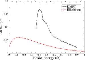
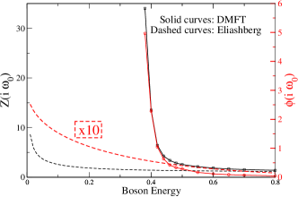
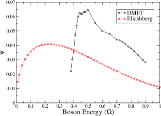
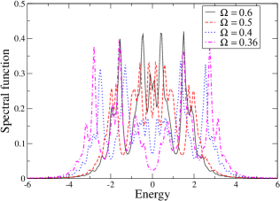
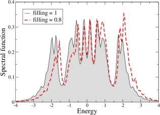
Fig. 2(a) shows the (half) superconducting gap as a function of Boson energy at the half filling. The electron-boson coupling is fixed at . We find that there exists an optimal Boson energy for the superconducting gap, which is around for these parameters. The ME theory, although resulting in different numerical values, exhibits the same non-monotonous behavior, with the optimal Boson energy at . To analyze the origin of the non-monotonous behavior, Fig. 2(b) shows and (whose ratio determines the gap amplitude) as a function of Boson energies. The ME theory results in the similar but milder and behavior. At very large (), both polaron and superconducting effects are weak ( and ), because the Boson energy is too large and has little effects on the ground state property. When decreases, both and increase, but at different rates. At larger (), grows faster, leading to increasing gap amplitudes. At smaller (), grows faster, leading to decreasing gap amplitudes. As (only obtained using ME theory), both and diverge, with the former being much faster. From our discussion in Section II.D, the decreasing superconducting gap below is the consequence that the polaron effect starts to dominate over the superconductivity at small . Fig. 3 provides the pairing amplitude as a function of the Boson energy , and the shape similar the superconducting gap is seen. The spectral functions at half filling for are provided in Fig. 4(a). As the Boson energy decreases, the spectral function first develops a dip Zer around the Fermi energy, indicating the superconducting state, and then keeps on decreasing in value due to the increasing polaron effect [ in Fig. 2(b)]. We emphasize that both and lead to a reduction in the spectral function near , and it is not easy to distinguish the polaron from the superconducting effect from the spectral function alone. An explicit evaluation of and to separate these two effects. To confirm that the dip around zero for is indeed caused by the superconductivity, not by the error caused by including only five bath orbitals, Fig. 4(b) presents the spectral function computed at band filling of 0.8. A dip around zero is also clearly observed.
III.2 Limitations of solvers and comparison to other methods
There are two dimensionless parameters that govern the validity of the ME theory – one and . The former is derived from the Midgal theory Migdal (1958); Grimvall (1981); Allen and Mitrovic (1983) which gives the condition where the vertex correction can be neglected; the later is obtained from DMFT Benedetti and Zeyher (1998); Deppeler and Millis (2002), and is proportional to obtained from ME theory Allen and Mitrovic (1983). Both parameters have to be small for ME theory to work. Roughly, the small guarantees the correct ground state, and the small gives the correct excitations Deppeler and Millis (2002). Note that small implies that ME theory is not valid for any given at small enough . As DMFT becomes exact in the infinite-dimension limit, we use it as a reference to see when and how the ME theory breaks down. As expected, the gaps obtained from ME theory and DMFT become closer when is small (larger at a given ). When is large, ME theory does not properly capture the polaron effect and thus gives the (wrong) superconducting ground state. Without considering the superconducting solution, Ref. Benedetti and Zeyher (1998) determines the critical value is of order one, above which the system becomes insulating. From Fig. 2(a) and Fig. 3, we see that below , the superconducting amplitude becomes negligible and the system is in the polaron state. As the ME theory predicts the superconducting state for all , our calculation results in a , above which the ME theory gives the wrong ground state. We have done the calculations for , 0.4 and 0.5 (not shown), and the resulting are all around 1. Our DMFT calculations thus extend the criterion given in Refs. Benedetti and Zeyher (1998); Deppeler and Millis (2002) to the superconducting solution.
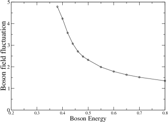
We also examine the harmonic Boson potential at small . We first represent the Boson field as a simple harmonic oscillator, i.e. (the convention is used), with a distortion field. In this representation the distortion , and characterizes the distortion fluctuation. as a function of is given in Fig. 5, which clearly shows a divergent behavior at small . Note that the diverging behavior in and [Fig. 2(b)], and the diverging behavior of [Fig. 5] happen at the same , which signals the polaron insulating phase. When is comparable to the lattice constant or the inter-electron distance, the validity of the quadratic potential may not be sufficient.
We now compare our results to those in the literature. We first discuss the DMFT results using other impurity solvers, including the Hirsch-Fye Hirsch and Fye (1986) Quantum Monte Carlo (QMC) Freericks et al. (1993); Freericks and Jarrell (1994, 1995), the second order perturbation in phonon propagators Freericks and Jarrell (1994), the semiclassical solver Millis et al. (1996); Lin and Millis (2009), the path integral Benedetti and Zeyher (1998), the diagrammatic expansion Deppeler and Millis (2002), and the continuous-time QMC Gull et al. (2011); Murakami et al. (2014). The Hirsch-Fye QMC is formally exact, and works efficiently at high temperature Freericks et al. (1993); Freericks and Jarrell (1994, 1995). The critical temperatures for charge density wave (CDW) and superconducting phases are determined by the divergence of the corresponding susceptibilities. The ED solver used here is for zero-temperature phases, and a direct comparison cannot be made. An investigation on CDW order at zero temperature is worthwhile. We notice that in the large limit, DMFT yields the polaron insulating solution, which can easily lead some CDW order as the local occupation prefers either zero or two electrons. In this sense, the DMFT phase diagram is consistent with the results from the QMC calculation, where the CDW phase happens at small regime whereas superconductivity at large regime Freericks et al. (1993). The semiclassical solver Millis et al. (1996); Lin and Millis (2009) neglects the Boson dynamics, and captures only the polaron but not the superconducting physics. The analysis based on path integral Benedetti and Zeyher (1998) and diagrammatic expansion Deppeler and Millis (2002) identifies an important dimensionless parameter , and our results (discussed in the first paragraph in this Section) are fully consistent with these results. In the parameter regime where both and are comparable to the bandwidth, the bipolaron effect becomes important Alexandrov et al. (1986), and several phases such as supersolid, CDW, and superconducting states, along with a quantum critical point are obtained Murakami et al. (2014). We do not explore the parameter regime, but it is the regime where the ED solver is applicable. Finally we note that in the two-dimensional electronic system, a weak electron-phonon coupling can lead to the CDW order that can coexist with the superconducting state Scalettar et al. (1989); Vekić et al. (1992); Sykora et al. (2009). The CDW order exhibited in this case originates mainly from the nesting of the band, but has nothing to do with the specific form the local interaction.
III.3 Connection to the recent high-pressure experiment
In 2015, Drozdov et. al. shows that applying a high pressure to on sulfur hydride (H2S) can enhance the superconducting up to 203K, and the isotope effect (replacing hydrogen by deuterium and tritium reduces ) further confirms that it is the phonon-mediated conventional superconductor Drozdov et al. (2015). One of their findings is that there is an optimal pressure for the superconductivity, above which the superconducting starts to decrease. Our calculation suggests a simple explanation for this non-monotonous behavior as a function of pressure, under the following three (reasonable) assumptions: (i) the Boson energy considered in the Holstein model corresponds to the Debye frequency (multiplied by ); (ii) applying a pressure increases the Debye frequency; and (iii) the electron-phonon coupling does not change significantly (within 10) upon applying the pressure. The isotope effect, which lowers the Debye frequency via increasing the atomic masses, lowers the superconducting . This well-known behavior corresponds to the Boson energy smaller than the optimal . When the applied pressure is too large such that the Debye frequency passes its optimal value, the superconducting again decreases. We emphasize that the optimal pressure can also be caused by other physics – for example, the Coulomb repulsion becomes stronger upon increasing the pressure, and leads to a reduction of superconducting . Our calculation cannot tell which one is the main mechanism. However, it does imply that an optimal pressure exists even without invoking the Coulomb repulsion. To quantitatively see how superconductivity is affected by a Hubbard is worthy of further investigations.
IV Conclusion
In this work we examine the superconducting solution in the Holstein model with semicircular density of states, using both the Migdal-Eliashberg theory and Dynamical Mean Field theory. The impurity model associated with DMFT is solved using the exact diagonalization. Although different in numerical values, both methods imply that for a given electron-Boson coupling there exists an optimal Boson energy for superconductivity. By analyzing the Green’s function, this non-monotonous behavior originates from the interplay between superconducting and polaron effects. At large , the polaron effect is small so the superconducting gap increases upon lowering . Below certain , the polaron effect starts to dominate and therefore reduces the superconductivity by making the system less metallic (reducing the DOS around the Fermi energy). In terms of many-body solvers, our DMFT results explicitly confirm that in the small limit, the ME theory breaks down by getting the wrong ground state. This result was already obtained in the calculations without breaking symmetries Benedetti and Zeyher (1998); Deppeler and Millis (2002), and here we extend this statement to the superconducting solution. Our calculation provides a simple explanation on the recent experiment on sulfur hydride, where a optimal pressure for the superconductivity was observed Drozdov et al. (2015). Searching Boson degrees of freedom (other than the phonons) to mediate the electron-electron attraction can be a promising approach to enhance the superconducting temperature.
Acknowledgement
We thank Qi Chen and Prabhakar Bandaru for helpful discussions, and Andrew Millis for very insightful comments.
References
- Onnes (1911) H. K. Onnes, Commun. Phys. Lab. Univ. Leiden: 120b (1911).
- Cooper (1956) L. N. Cooper, Phys. Rev. 104, 1189 (1956), URL http://link.aps.org/doi/10.1103/PhysRev.104.1189.
- Bardeen et al. (1957a) J. Bardeen, L. N. Cooper, and J. R. Schrieffer, Phys. Rev. 106, 162 (1957a), URL http://link.aps.org/doi/10.1103/PhysRev.106.162.
- Bardeen et al. (1957b) J. Bardeen, L. N. Cooper, and J. R. Schrieffer, Phys. Rev. 108, 1175 (1957b), URL http://link.aps.org/doi/10.1103/PhysRev.108.1175.
- Kirzhnits et al. (1973) D. Kirzhnits, E. Maksimov, and D. Khomskii, Journal of Low Temperature Physics 10, 79 (1973), ISSN 0022-2291, URL http://dx.doi.org/10.1007/BF00655243.
- Mann (2011) A. Mann, Nature 475, 280 (2011).
- Bednorz and Müller (1986) J. G. Bednorz and K. A. Müller, Zeitschrift für Physik B Condensed Matter 64, 189 (1986), ISSN 1431-584X, URL http://dx.doi.org/10.1007/BF01303701.
- Damascelli et al. (2003) A. Damascelli, Z. Hussain, and Z.-X. Shen, Rev. Mod. Phys. 75, 473 (2003), URL http://link.aps.org/doi/10.1103/RevModPhys.75.473.
- Kamihara et al. (2006) Y. Kamihara, H. Hiramatsu, M. Hirano, R. Kawamura, H. Yanagi, T. Kamiya, and H. Hosono, JACS 128, 10012 (2006), eprint http://dx.doi.org/10.1021/ja063355c, URL http://dx.doi.org/10.1021/ja063355c.
- Kamihara et al. (2008) Y. Kamihara, T. Watanabe, M. Hirano, and H. Hosono, JACS 130, 3296 (2008), eprint http://dx.doi.org/10.1021/ja800073m, URL http://dx.doi.org/10.1021/ja800073m.
- Ge et al. (2015) J.-F. Ge, Z.-L. Liu, C. Liu, C.-L. Gao, D. Qian, Q.-K. Xue, Y. Liu, and J.-F. Jia, Nat Mater 14, 285 (2015), URL http://dx.doi.org/10.1038/nmat4153.
- Dagotto (1994) E. Dagotto, Rev. Mod. Phys. 66, 763 (1994).
- Imada et al. (1998) M. Imada, A. Fujimori, and Y. Tokura, Rev. Mod. Phys. 70, 1039 (1998), URL http://link.aps.org/doi/10.1103/RevModPhys.70.1039.
- Hosono et al. (2015) H. Hosono, K. Tanabe, E. Takayama-Muromachi, H. Kageyama, S. Yamanaka, H. Kumakura, M. Nohara, H. Hiramatsu, and S. Fujitsu, Science and Technology of Advanced Materials 16, 033503 (2015), URL http://stacks.iop.org/1468-6996/16/i=3/a=033503.
- Eliashberg (1960) G. M. Eliashberg, JEPT 11, 696 (1960).
- Migdal (1958) A. B. Migdal, JEPT 7, 996 (1958).
- Morel and Anderson (1962) P. Morel and P. W. Anderson, Phys. Rev. 125, 1263 (1962), URL http://link.aps.org/doi/10.1103/PhysRev.125.1263.
- Allen and Dynes (1975) P. B. Allen and R. C. Dynes, Phys. Rev. B 12, 905 (1975), URL http://link.aps.org/doi/10.1103/PhysRevB.12.905.
- Bergmann and Rainer (1973) G. Bergmann and D. Rainer, Z. Phys. 263, 59 (1973).
- Grimvall (1981) G. Grimvall, The electron-phonon interaction in metal (North-Holland Publishing Company, 1981).
- Allen and Mitrovic (1983) P. B. Allen and B. Mitrovic, Solid State Physics 37, 1 (1983).
- McMillan (1968) W. L. McMillan, Phys. Rev. 167, 331 (1968), URL http://link.aps.org/doi/10.1103/PhysRev.167.331.
- Drozdov et al. (2015) A. P. Drozdov, M. I. Eremets, I. A. Troyan, V. Ksenofontov, and S. I. Shylin, Nature 525, 73 (2015), URL http://dx.doi.org/10.1038/nature14964.
- Qing-Yan et al. (2012) W. Qing-Yan, L. Zhi, Z. Wen-Hao, Z. Zuo-Cheng, Z. Jin-Song, L. Wei, D. Hao, O. Yun-Bo, D. Peng, C. Kai, et al., Chin. Phys. Lett. 29, 037402 (2012), URL http://stacks.iop.org/0256-307X/29/i=3/a=037402.
- Lee et al. (2014) J. J. Lee, F. T. Schmitt, R. G. Moore, S. Johnston, Y.-T. Cui, W. Li, M. Yi, Z. K. Liu, M. Hashimoto, Y. Zhang, et al., Nature 515, 245 (2014).
- Rademaker et al. (2016) L. Rademaker, Y. Wang, T. Berlijn, and S. Johnston, New Journal of Physics 18, 022001 (2016), URL http://stacks.iop.org/1367-2630/18/i=2/a=022001.
- Wang et al. (2016) Y. Wang, K. Nakatsukasa, L. Rademaker, T. Berlijn, and S. Johnston, Superconductor Science and Technology 29, 054009 (2016), URL http://stacks.iop.org/0953-2048/29/i=5/a=054009.
- Smolyaninova et al. (2014) V. N. Smolyaninova, B. Yost, K. Zander, M. S. Osofsky, H. Kim, S. Saha, R. L. Greene, and I. I. Smolyaninov, Sci. Rep. 4, 7321 (2014), URL http://dx.doi.org/10.1038/srep07321.
- Smolyaninov and Smolyaninova (2015) I. I. Smolyaninov and V. N. Smolyaninova, Phys. Rev. B 91, 094501 (2015), URL http://link.aps.org/doi/10.1103/PhysRevB.91.094501.
- Holstein (1959) T. Holstein, Ann. Phys. 8, 325 (1959).
- Georges et al. (1996) A. Georges, G. Kotliar, W. Krauth, and M. J. Rozenberg, Rev. Mod. Phys. 68, 13 (1996).
- Kotliar and Vollhardt (2004) G. Kotliar and D. Vollhardt, Physics Today 57 (2004).
- Maier et al. (2005) T. Maier, M. Jarrell, T. Pruschke, and M. H. Hettler, Rev. Mod. Phys. 77, 1027 (2005).
- Gull et al. (2011) E. Gull, A. J. Millis, A. I. Lichtenstein, A. N. Rubtsov, M. Troyer, and P. Werner, Rev. Mod. Phys. 83, 349 (2011), URL http://link.aps.org/doi/10.1103/RevModPhys.83.349.
- Freericks et al. (1993) J. K. Freericks, M. Jarrell, and D. J. Scalapino, Phys. Rev. B 48, 6302 (1993), URL http://link.aps.org/doi/10.1103/PhysRevB.48.6302.
- Freericks and Jarrell (1994) J. K. Freericks and M. Jarrell, Phys. Rev. B 50, 6939 (1994), URL http://link.aps.org/doi/10.1103/PhysRevB.50.6939.
- Freericks and Jarrell (1995) J. K. Freericks and M. Jarrell, Phys. Rev. Lett. 75, 2570 (1995), URL http://link.aps.org/doi/10.1103/PhysRevLett.75.2570.
- Benedetti and Zeyher (1998) P. Benedetti and R. Zeyher, Phys. Rev. B 58, 14320 (1998), URL http://link.aps.org/doi/10.1103/PhysRevB.58.14320.
- Deppeler and Millis (2002) A. Deppeler and A. J. Millis, Phys. Rev. B 65, 224301 (2002), URL http://link.aps.org/doi/10.1103/PhysRevB.65.224301.
- Wellein and Fehske (1997) G. Wellein and H. Fehske, Phys. Rev. B 56, 4513 (1997), URL http://link.aps.org/doi/10.1103/PhysRevB.56.4513.
- Kalosakas et al. (1998) G. Kalosakas, S. Aubry, and G. P. Tsironis, Phys. Rev. B 58, 3094 (1998), URL http://link.aps.org/doi/10.1103/PhysRevB.58.3094.
- Meyer et al. (2002) D. Meyer, A. C. Hewson, and R. Bulla, Phys. Rev. Lett. 89, 196401 (2002), URL http://link.aps.org/doi/10.1103/PhysRevLett.89.196401.
- Werner and Millis (2007) P. Werner and A. J. Millis, Phys. Rev. Lett. 99, 146404 (2007), URL http://link.aps.org/doi/10.1103/PhysRevLett.99.146404.
- De Filippis et al. (2012) G. De Filippis, V. Cataudella, E. A. Nowadnick, T. P. Devereaux, A. S. Mishchenko, and N. Nagaosa, Phys. Rev. Lett. 109, 176402 (2012), URL http://link.aps.org/doi/10.1103/PhysRevLett.109.176402.
- Murakami et al. (2015) Y. Murakami, P. Werner, N. Tsuji, and H. Aoki, Phys. Rev. B 91, 045128 (2015), URL http://link.aps.org/doi/10.1103/PhysRevB.91.045128.
- Vekić et al. (1992) M. Vekić, R. M. Noack, and S. R. White, Phys. Rev. B 46, 271 (1992), URL http://link.aps.org/doi/10.1103/PhysRevB.46.271.
- Sykora et al. (2009) S. Sykora, A. Hübsch, and K. W. Becker, EPL (Europhysics Letters) 85, 57003 (2009), URL http://stacks.iop.org/0295-5075/85/i=5/a=57003.
- Hague (2005) J. P. Hague, Journal of Physics: Condensed Matter 17, 5663 (2005), URL http://stacks.iop.org/0953-8984/17/i=37/a=005.
- Murakami et al. (2014) Y. Murakami, P. Werner, N. Tsuji, and H. Aoki, Phys. Rev. Lett. 113, 266404 (2014), URL http://link.aps.org/doi/10.1103/PhysRevLett.113.266404.
- Kotliar et al. (2006) G. Kotliar, S. Y. Savrasov, K. Haule, V. S. Oudovenko, O. Parcollet, and C. A. Marianetti, Rev. Mod. Phys. 78, 865 (2006).
- Liebsch and Ishida (2012) A. Liebsch and I. Ishida, Journal of Physics: Condensed Matter 24 (2012).
- Lin and Demkov (2013) C. Lin and A. A. Demkov, Phys. Rev. B 88, 035123 (2013), URL http://link.aps.org/doi/10.1103/PhysRevB.88.035123.
- Zgid et al. (2012) D. Zgid, E. Gull, and G. K.-L. Chan, Phys. Rev. B 86, 165128 (2012).
- Lin and Demkov (2014) C. Lin and A. A. Demkov, Phys. Rev. B 90, 235122 (2014), URL http://link.aps.org/doi/10.1103/PhysRevB.90.235122.
- Go and Millis (2015) A. Go and A. J. Millis, Phys. Rev. Lett. 114, 016402 (2015), URL http://link.aps.org/doi/10.1103/PhysRevLett.114.016402.
- Lin and Demkov (2015) C. Lin and A. A. Demkov, Phys. Rev. B 92, 155135 (2015), URL http://link.aps.org/doi/10.1103/PhysRevB.92.155135.
- Millis et al. (1996) A. J. Millis, R. Mueller, and B. I. Shraiman, Phys. Rev. B 54, 5389 (1996), URL http://link.aps.org/doi/10.1103/PhysRevB.54.5389.
- Okamoto et al. (2005) S. Okamoto, A. Fuhrmann, A. Comanac, and A. J. Millis, Phys. Rev. B 71, 235113 (2005), URL http://link.aps.org/doi/10.1103/PhysRevB.71.235113.
- Lin and Millis (2009) C. Lin and A. J. Millis, Phys. Rev. B 79, 205109 (2009), URL http://link.aps.org/doi/10.1103/PhysRevB.79.205109.
- Mahan (2000) G. D. Mahan, Many-Particle Physics 3rd edition (Kluwer Academic/Plenum publisher, New York, 2000).
- (61) Due to the small number of bath orbitals, the zero DOS cannot be observed in the calculation.
- Hirsch and Fye (1986) J. E. Hirsch and R. M. Fye, Phys. Rev. Lett. 56, 2521 (1986), URL http://link.aps.org/doi/10.1103/PhysRevLett.56.2521.
- Alexandrov et al. (1986) A. S. Alexandrov, J. Ranninger, and S. Robaszkiewicz, Phys. Rev. B 33, 4526 (1986), URL http://link.aps.org/doi/10.1103/PhysRevB.33.4526.
- Scalettar et al. (1989) R. T. Scalettar, N. E. Bickers, and D. J. Scalapino, Phys. Rev. B 40, 197 (1989), URL http://link.aps.org/doi/10.1103/PhysRevB.40.197.