Theory of population coupling and applications to describe high order correlations in large populations of interacting neurons

Abstract

To understand the collective spiking activity in neuronal populations, it is essential to reveal basic circuit variables responsible for these emergent functional states. Here, I develop a mean field theory for the population coupling recently proposed in the studies of visual cortex of mouse and monkey, relating the individual neuron activity to the population activity, and extend the original form to the second order, relating neuron-pair’s activity to the population activity, to explain the high order correlations observed in the neural data. I test the computational framework on the salamander retinal data and the cortical spiking data of behaving rats. For the retinal data, the original form of population coupling and its advanced form can explain a significant fraction of two-cell correlations and three-cell correlations, respectively. For the cortical data, the performance becomes much better, and the second order population coupling reveals non-local effects in local cortical circuits.

I Introduction

To uncover the neural circuit mechanisms underlying animal behavior, e.g., working memory or decision making, is a fundamental issue in systems neuroscience [1, 2]. Recent developments in multi-neuron recording methods make simultaneous recording of neuronal population activity possible, which gives rise to the challenging computational tasks of finding basic circuit variables responsible for the observed collective behavior of neural populations [3]. The collective behavior arises from interactions among neurons, and forms the high dimensional neural code. To search for a low dimensional and yet neurobiologically plausible representation of the neural code, thus becomes a key step to understand how the collective states generate behavior and cognition.

Correlations among neurons’ spiking activities play a prominent role in deciphering the neural code [4]. Various models were proposed to understand the pairwise correlations in the population activity [5, 6, 7]. Modeling these correlations sheds light on the functional organization of the nervous system [8]. However, as the population size grows, higher order correlations have to be taken into account for modeling synchronous spiking events, which are believed to be crucial for neural information transmission [9, 10, 11]. In addition, the conclusion drawn from small size populations may not be correct for large size populations. Theoretical studies have already proved that high order interactions among neurons are necessary for generating widespread population activity [12, 13]. However, introduction of high order multi-neuron couplings always suffers from a combinatorial explosion of model parameters to be estimated from the finite neural spike train data.

To account for high order correlations, various models with different levels of approximation were proposed, for example, the reliable interaction model [14] with the main caveat that the rare patterns are discarded during inference of the coupling terms, the dichotomized Gaussian model [7, 15] in which correlations among neurons are caused by common Gaussian inputs to threshold neurons, the K-pairwise model [16, 17] in which an effective potential related to the synchronous firing of $K$ neurons was introduced, yet hard to be interpreted in terms of functional connectivity, and the restricted Boltzmann machine [18] where hidden units were shown to be capable of capturing high order dependences but their number should be predefined and difficult to infer from the data [19]. One can also take into account part of the statistical features of the population activity (e.g., simultaneous silent neural pattern) and assume homogeneity for high order interactions among neurons due to the population size limitation [20]. In this paper, I provide a low dimensional neurobiological model for describing the high order correlations and extracting useful information about neural functional organization and population coding.

In this study, I interpret correlations in terms of population coupling, a concept recently proposed to understand the multi-neuron firing patterns of the visual cortex of mouse and monkey [21]. The population coupling characterizes the relationship of the activity of a single neuron with the population activity; this is because, the firing of one neuron is usually correlated with the firing pattern of other neurons. I further generalize the original population coupling to its higher order form, i.e., the relationship of pairwise firing with the population activity. I then derive the practical dimensionality reduction method for both types of population couplings, and test the method on different types of neural data, including ganglion cells in the salamander retina onto which a repeated natural movie was projected [17], and layer 2/3 as well as layer 5 cortical cells in the medial prefrontal cortex (MPC) of behaving rats [22].

In this paper, I develop a theoretical model of population coupling and its advanced form, to explain higher order correlations in the neural data. Methodologically, I propose the fast mean field method not only to learn the population couplings but also to evaluate the high order correlations. Note that this is computationally hard in a traditional maximum entropy model by using sampling-based method. Conceptually, I generalize the normal population coupling by introducing the second-order population coupling, which reveals interesting features from the data. First, it can explain a significant amount of three-cell correlations, and it works much better in cortical data than in retinal data. Second, the second-order population coupling matrix has distinct features in retinal and cortical data. The cortical one shows clear stripe-like structure while the retinal one has no such apparent structure. Altogether, this work marks a major step to understand the low-order representation of complex neural activity in both concepts and methods.

II Model description and mean-field methods

For a neuronal population of size $N$, the neural spike trains of duration $T$ are binned with temporal resolution $\tau$, yielding $M=\lceil T/\tau\rceil$ samples of $N$-dimensional binary neural firing patterns. I use $s_{i}=+1$ to denote firing state of neuron $i$, and $s_{i}=-1$ for silent state. Neural responses to repeated stimulus (or the same behavioral tasks) vary substantially (so-called trial-to-trial variability) [23, 24]. To model the firing pattern statistics, I assign each firing pattern $\mathbf{s}$ a cost function (energy in statistical physics jargon) $E(\mathbf{s})$, then the probability of observing one pattern $\mathbf{s}$ can be written as $P(\mathbf{s})\propto\exp(-E(\mathbf{s}))$, where

$$E(\mathbf{s})=-\sum_{i}h_{i}s_{i}-\sum_{i}J_{i}s_{i}\Biggl{(}\sum_{j\neq i}s_{j}\Biggr{)}.$$ (1)

This is the first low dimensional representation to be studied. High energy state $\mathbf{s}$ corresponds to low probability of observation. $h_{i}$ is the firing bias constraining the firing rate of neuron $i$, while $J_{i}$ characterizes how strongly neuron $i$’s spiking activity correlates with the population activity measured by the sum of other neurons’ activity. I name $J_{i}$ the first order population coupling (${\rm PopC}_{1}$). Thus, only $2N$ parameters needs to be estimated from the neural data. This number of model parameters is much less than that in conventional maximum entropy model [17].

To model the high order correlation (e.g., three neuron firing correlation), I further generalize ${\rm PopC}_{1}$ to its advanced form, i.e., the second order population coupling, namely ${\rm PopC}_{2}$, describing the relationship of pairwise firing with the population activity, and the corresponding energy is given by

$$E(\mathbf{s})=-\sum_{i}h_{i}s_{i}-\sum_{i<j}w_{ij}s_{i}s_{j}\Biggl{(}\sum_{k\neq i,j}s_{k}\Biggr{)},$$ (2)

where $w_{ij}$ characterizes how strongly the firing state of the neuron pair $(ij)$ correlates with the firing activities of other neurons. This term is expected to increase the prediction ability for modeling high order correlations in the neural data. Under the framework of ${\rm PopC}_{2}$, the total number of parameters to be estimated from the data is $N+N(N-1)/2$. ${\rm PopC}_{1}$ and ${\rm PopC}_{2}$ have a clear neurobiological interpretation (for ${\rm PopC}_{1}$, see a recent study [21], and the results obtained under the ${\rm PopC}_{2}$ can also be experimentally tested), and moreover they can be interpreted in terms of functional interactions among neurons (as shown later).

To find the model parameters as a low dimensional representation, I apply the maximum likelihood learning principle corresponding to maximizing the log-likelihood $\ln P(\mathbf{s})$ with respect to the parameters. The learning equation for ${\rm PopC}_{1}$ is given by

$$h_{i}^{t+1} =h_{i}^{t}+\eta\Biggl{(}\Bigl{<}s_{i}\Bigr{>}_{{\rm data}}-\Bigl{<}s_{i}\Bigr{>}_{{\rm model}}\Biggr{)},$$ (3a)

$$J_{i}^{t+1} =J_{i}^{t}+\eta\Biggl{(}\sum_{j\neq i}\Bigl{<}s_{i}s_{j}\Bigr{>}_{{\rm data}}-\sum_{j\neq i}\Bigl{<}s_{i}s_{j}\Bigr{>}_{{\rm model}}\Biggr{)},$$ (3b)

where $t$ and $\eta$ denote the learning step and learning rate, respectively. The maximum likelihood learning shown here has a simple interpretation of minimizing the Kullback-Leibler divergence between the observation probability and the model probability [25, 26]. In an analogous way, one gets the learning equation for ${\rm PopC}_{2}$,

$$w_{ij}^{t+1}=w_{ij}^{t}+\eta\Biggl{(}\sum_{k\neq i,j}\Bigl{<}s_{i}s_{j}s_{k}\Bigr{>}_{{\rm data}}-\sum_{k\neq i,j}\Bigl{<}s_{i}s_{j}s_{k}\Bigr{>}_{{\rm model}}\Biggr{)}.$$ (4)

In the learning equations Eq. (3) and Eq. (4), the data dependent terms can be easily computed from the binned neural data. However, the model expectations of the firing rate (magnetization in statistical physics) and correlations are quite hard to evaluate without any approximations. Here I use the mean field method to tackle this difficulty.

First, I write the energy term into a unified form,

$$E(\mathbf{s})=-\sum_{i}h_{i}s_{i}-\sum_{a}\Gamma_{a}\prod_{i\in\partial a}s_{i},$$ (5)

where $a$ denotes the interaction index and $\partial a$ denotes the neuron set involved in the interaction $a$. $a=(ij)$ for ${\rm PopC}_{1}$ and $(ijk)$ for ${\rm PopC}_{2}$. Therefore, ${\rm PopC}_{1}$ introduces the pairwise interaction as $\Gamma_{ij}=J_{i}+J_{j}$, while ${\rm PopC}_{2}$ introduces the triplet interaction as $\Gamma_{ijk}=w_{ij}+w_{jk}+w_{ik}$. The multi-neuron interaction in the conventional Ising model is decomposed into first order or second order population coupling terms. This decomposition still maintains the functional heterogeneity of single neurons or neuron pairs, but reduces drastically the dimensionality of the neural representation for explaining high order correlations. In principle, one can combine ${\rm PopC}_{1}$ and ${\rm PopC}_{2}$ to predict both pairwise and triplet correlations. However, in this work, I focus on the pure effect of each type of population coupling.

In fact, the conventional Ising model [27] can be recovered by setting $\Gamma_{ij}=J_{ij}$, which is pairwise interaction. The learning equation is derived similarly, and is run by reducing the deviation between the model pairwise correlation and the clamped one (computed from the data) [28].

Second, the statistical properties of the model (Eq. 5) can be analyzed by the cavity method in the mean field theory [29]. The self-consistent equations are written in the form of message passing (detailed derivations were given in Refs [30, 31], see also Appendix A) as

$$m_{i\rightarrow a} =\tanh\left(h_{i}+\sum_{b\in\partial i\backslash a}\tanh^{-1}\hat{m}_{b\rightarrow i}\right),$$ (6a)

$$\hat{m}_{b\rightarrow i} =\tanh\Gamma_{b}\prod_{j\in\partial b\backslash i}m_{j\rightarrow b},$$ (6b)

where $\partial b\backslash i$ denotes the member of interaction $b$ except $i$, and $\partial i\backslash a$ denotes the interaction set $i$ is involved in with $a$ removed. $m_{i\rightarrow a}$ is interpreted as the message passing from the neuron $i$ to the interaction $a$ it participates in, while $\hat{m}_{b\rightarrow i}$ is interpreted as the message passing from the interaction $b$ to its member $i$. This iteration equation is also called the belief propagation (BP), which serves as the message passing algorithm for the statistical inference of the model parameters. Iteration of the message passing equation on the inferred model would converge to a fixed point corresponding to a global minimum of the free energy (in the cavity method approximation [31])

$$F\equiv-\ln Z=-\sum_{i}\ln Z_{i}+\sum_{a}(|\partial a|-1)\ln Z_{a},$$ (7)

where $Z$ is the normalization constant of the model probability $P(\mathbf{s})$. The free energy contribution of one neuron is $-\ln Z_{i}=-\ln\sum_{x=\pm 1}\mathcal{H}_{i}(x)$ and the free energy contribution of one interaction is $-\ln Z_{a}=-\ln\cosh\Gamma_{a}-\ln\left(1+\tanh\Gamma_{a}\prod_{i\in\partial a}m_{i\rightarrow a}\right)$. I define the function $\mathcal{H}_{i}(x)\equiv e^{xh_{i}}\prod_{b\in\partial i}\cosh\Gamma_{b}(1+x\hat{m}_{b\rightarrow i})$. At the same time, the model firing rate and multi-neuron correlation can be estimated as

$$m_{i} =\tanh\left(h_{i}+\sum_{b\in\partial i}\tanh^{-1}\hat{m}_{b\rightarrow i}\right),$$ (8a)

$$C_{a} =\frac{\tanh\Gamma_{a}+\prod_{i\in\partial a}m_{i\rightarrow a}}{1+\tanh\Gamma_{a}\prod_{i\in\partial a}m_{i\rightarrow a}}.$$ (8b)

Magnetization and correlation are defined as $m_{i}=\left<s_{i}\right>$ and $C_{a}=\left<\prod_{i\in\partial a}s_{i}\right>$, respectively.

A brief derivation of Eq. (8) is given in Appendix A. Here the multi-neuron correlation is calculated directly from the cavity method approximation and expected to be accurate enough for current neural data analysis [28]. This is because, correlations under the model are evaluated taking into account nearest-neighbor interactions, rather than naive full independence among neurons. This approximation is expected to work well in a weakly-correlated neural population [5, 8], where long-range strong correlations do not develop. A similar application of this principle revealed a non-trivial geometrical structure of population codes in salamander retina [28]. Another advantage is the low computation cost. Both the free energy and the pairwise correlations can be estimated by the time complexity of the order $\mathcal{O}(N^{2})$ for ${\rm PopC}_{1}$, and $\mathcal{O}(N^{3})$ for triplet correlations in ${\rm PopC}_{2}$, which is one order of magnitude lower than the tractable model of ${\rm PopC}_{1}$ recently proposed in Ref. [32]. A more accurate expression could be derived from linear response theory [33] with much more expensive computational cost (increased by an order of magnitude ($\mathcal{O}(N)$).

To estimate the information carried by a neural population, one needs to compute the entropy, which is defined as $S=-\sum_{\mathbf{s}}P(\mathbf{s})\ln P(\mathbf{s})$, and it measures the capacity of the neural population for information transmission. The more obvious variability the neural responses have, the larger the entropy value is. The entropy of the model can be estimated from the fixed point of the message passing equation. Based on the standard thermodynamic relation, $S=-F+E$, where $E$ is the energy of the neural population and given by

$$E =-\sum_{i}\Delta E_{i}+\sum_{a}(|\partial a|-1)\Delta E_{a},$$ (9a)

$$\Delta E_{i} =\frac{h_{i}\sum_{x=\pm 1}x\mathcal{H}_{i}(x)+\sum_{x=\pm 1}\mathcal{G}_{i}(x)}{\sum_{x=\pm 1}\mathcal{H}_{i}(x)},$$ (9b)

$$\Delta E_{a} =\Gamma_{a}\frac{\tanh\Gamma_{a}+\prod_{i\in\partial a}m_{i\rightarrow a}}{1+\tanh\Gamma_{a}\prod_{i\in\partial a}m_{i\rightarrow a}},$$ (9c)

$$\begin{split}\mathcal{G}_{i}(x)&=\sum_{b\in\partial i}e^{xh_{i}}\left[\Gamma_{b}\sinh\Gamma_{b}(1+x\hat{m}_{b\rightarrow i})+x\Gamma_{b}\cosh\Gamma_{b}(1-\tanh^{2}\Gamma_{b})\prod_{j\in\partial b\backslash i}m_{j\rightarrow b}\right]\\ &\times\prod_{a\in\partial i\backslash b}\cosh\Gamma_{a}(1+x\hat{m}_{a\rightarrow i}).\end{split}$$ (9d)

The basic procedure to infer population couplings is given as follows. At the beginning, all model parameters are assigned zero value. It is followed by three steps: ($i$) Messages are initialized randomly and uniformly in the interval $(-1,1)$. ($ii$) Eq. (6) are then run until converged, and the magnetizations as well as multi-neuron correlations are estimated using Eq. (8). ($iii$) The estimated magnetizations and correlations are used at each gradient ascent learning step (Eq. (3) or Eq. (4)). When one gradient learning step is finished, another step starts by repeating the above procedure (from ($i$) to ($iii$)). To learn the higher order population coupling, the damping technique is used to avoid oscillation behavior, i.e., $w_{{\rm new}}=\gamma w_{{\rm new}}+(1-\gamma)w_{{\rm old}}$ where $\gamma$ is the damping factor taking a small value.

The inferred model can also be used to generate the distribution of spike synchrony, i.e., the probability of $K$ simultaneous spikes. This distribution can be estimated by using Monte Carlo (MC) simulation on the model. The standard procedure goes as follows. The simulation starts from a random initial configuration $\mathbf{s}_{0}$, and tries to search for the low energy state, then the energy is lowered by a series of elementary updates, and for each elementary update, $N$ proposed neuronal state flips are carried out. That is, the transition probability from state $\mathbf{s}$ to $\mathbf{s}^{\prime}$ with only $s_{i}$ flipped ($s^{\prime}_{i}=-s_{i}$) is expressed as $e^{-2s_{i}H_{i}}$ where $H_{i}=h_{i}+\sum_{a\in\partial i}\Gamma_{a}\prod_{j\in\partial a\backslash i}s_{j}$. The equilibrium samples are collected after sufficient thermal equilibration. These samples (a total of $20000$ samples in simulations) are finally used to estimate the distribution of spike synchrony.

Figure 1: (Color online) Inference performances of ${\rm PopC}_{1}$ on the retinal data ($N=40$, one typical example). (A) Firing rate in the data is reproduced by the model. (B) Two-cell correlations are explained partially by ${\rm PopC}_{1}$ ($74.10\%$). A Monte-Carlo (MC) sampling of the model yields similar results to belief propagation (BP), which is much faster. (C) From the MC samples, three-cell correlations can also be estimated. (D) Probability of $K$ synchronous spiking under the model is compared with that of the data.

III Results

By using the mean field method, I first test both types of population couplings on the retina data, which is the spike train of $160$ ganglion cells in a small patch of the salamander retina [17]. The retina was stimulated with a repeated natural movie. The spike train data is binned with the bin size equal to $20ms$ reflecting the temporal correlation time scale, yielding about $282744$ binary firing patterns for data modeling.

I then test the same concepts on the cortical data of behaving rats. Rats performed the odor-place matching working memory during one task session, and spiking activities of $117$ cells in both superficial layer $2/3$ and deep layer (layer $5$) of medial prefrontal cortex were simultaneously recorded (for detailed experiments, see Ref. [22]). One task session consists of about $40$ trials, yielding a spike train of these cortical cells binned with the temporal resolution $\tau=20ms$ (a total of $140596$ firing patterns).

III.1 Inference performances on the retinal data

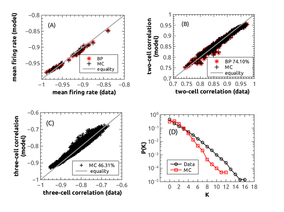
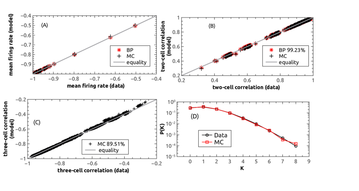
Fig. 1 reports the inference result on a network example of $40$ neurons selected randomly from the original dataset. The firing rate is predicted faithfully by the model using either MC or BP (Fig. 1 (A)). Inferring only ${\rm PopC}_{1}$, one could predict about $74.10\%$ of entire pairwise correlation (a precision criterion is set to $7.0\times 10^{-3}$ in this paper) (Fig. 1 (B)). This means that $74.10\%$ of the whole correlation set have the absolute value of the deviation between the predicted correlation and measured one ($|C_{a}^{{\rm pred}}-C_{a}^{{\rm ms}}|$) smaller than the precision criterion. Using the sampled configurations of neural firing activity from the MC simulation, one could also predict three-cell correlations (Fig. 1 (C)), whereas, the prediction fraction can be improved by a significant amount after introducing ${\rm PopC}_{2}$, as I shall show later. In addition, fitting only $2N$ model parameters in ${\rm PopC}_{1}$ analysis could not predict the tail of spike synchrony distribution (Fig. 1 (D)); this is expected as no higher order interaction terms are included in the model, and rare events of large $K$ spikes are also difficult to observe in a finite sampling during MC simulations.

Figure 2: (Color online) Inference performances of ${\rm PopC}_{2}$ on the retinal data ($N=40$, one typical example). (A) Firing rate in the data is reproduced by the model. (B) Three-cell correlations are explained partially by ${\rm PopC}_{2}$ ($64.44\%$). (C) Interaction matrix for ${\rm PopC}_{2}$. (D) Probability of $K$ synchronous spiking under the model is compared with that of the data.

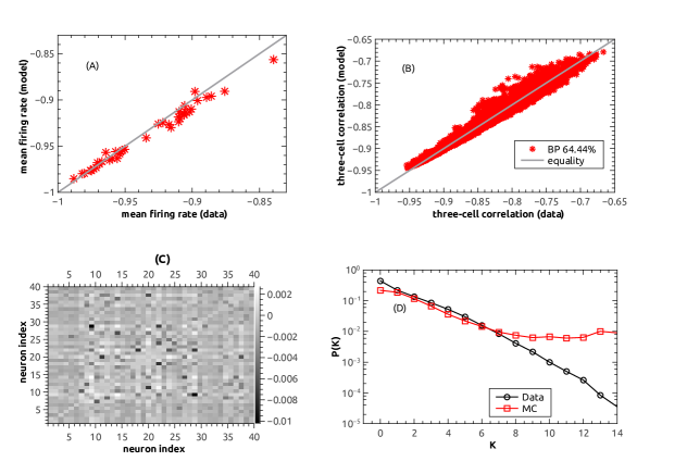
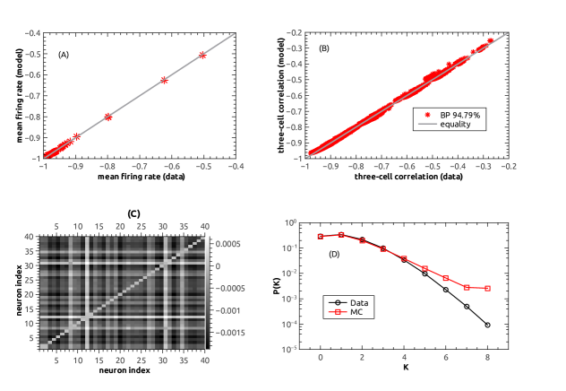
The inference results of ${\rm PopC}_{2}$ are given in Fig. 2. Note that, by considering the correlation between the pairwise firing activity and the global population activity, i.e., the second order population coupling, the three-cell correlation could be predicted partially ($64.44\%$), and this fraction is much larger than that of ${\rm PopC}_{1}$ (Fig. 1 (C)). This is due to the specific structure of ${\rm PopC}_{2}$, which incorporates explicitly three-cell correlations into the construction of couplings (Eq. (4)). Technically, the mean-field theory for ${\rm PopC}_{2}$ avoids the slow sampling and evaluates the high order correlations in a fast way. Alternatively, one could fit the data using the conventional Ising model [27] with the same number of model parameters as ${\rm PopC}_{2}$, whereas, the three-cell correlations are hard to predict using MC samplings, and a similar phenomenon was also observed in a previous work for modeling pairwise correlations [33]. Therefore I speculate that ${\rm PopC}_{2}$ acts as a key circuit variable for third order correlations.

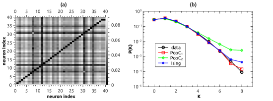
The interaction matrix of $\{w_{ij}\}$ reveals how important each pair of neurons is for the entire population activity (emergent functional state of the whole network). As shown in Fig. 2 (C), ${\rm PopC}_{2}$ matrix has no apparent structure of organization, i.e., each neuron can be paired with both positive and negative couplings. Some pairs have large negative ${\rm PopC}_{2}$, suggesting that these components are anti-correlated with the population activity. That is to say, the activity of these neuron-pairs is not synchronized to the population activity characterized by the summed activity over all neurons except these pairs. In the network, there also exist positive ${\rm PopC}_{2}$s, which shows that these neuron-pairs are positively correlated with the population in neural activity. The interaction matrix shown here may be related to the revealed overlapping modular structure of retinal neuron interactions [8, 14]. In this structure, neurons interact locally with their adjacent neurons, and in particular this feature is scalable and applicable for larger networks. It seems that one individual neuron does not impact directly the entire population, and a small group of neighboring neurons have similar visual feature selectivity [34]. This result is also consistent with two-neuron interaction map of the conventional Ising model (Fig. 3 (a)). Note that in functional interpretation, these two-neuron interactions are inherently different from ${\rm PopC}_{2}$, which is designed to explain high-order correlations by using less model parameters than necessary.

Figure 3: (Color online) Inference performances of Ising model on the retinal data ($N=40$, one typical example) compared with population coupling. (a) Two-neuron interaction matrix. (b) Probability of $K$ synchronous spiking under the model is compared with that of the data.

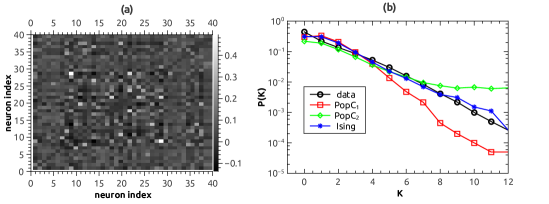
${\rm PopC}_{2}$ behaves better than ${\rm PopC}_{1}$ in predicting the spike synchrony distribution (Fig. 2 (D)) in the small $K$ regime (the prediction is improved from $K=4$ for ${\rm PopC}_{1}$ to $K=8$ for ${\rm PopC}_{2}$). An intuitive explanation is that ${\rm PopC}_{2}$ introduces equivalently triplet interactions among neurons, and it is known that high order interactions are necessary for generating widespread population activity [12]. However, ${\rm PopC}_{2}$ overestimates the distribution when rare events of synchronous spiking are considered. This may be related to the difficulty of obtaining sufficient equilibrium samples of the model, especially those samples with large population activity. The spike synchrony distribution is also compared with that obtained under Ising model (Fig. 3 (b)). Different performances are related to the multi-information measure of neural population explained below.

Figure 4: (Color online) Multi-information and prediction fraction of correlations under the simplified model for the retinal network. The result is averaged over $10$ network samples for each $N$. (a) Multi-information (in bits) versus the network size $N$. (b) The prediction fraction $\rho$ versus the network size. ${\rm PopC}_{1}$ is used to predict two-cell correlations, and ${\rm PopC}_{2}$ is used to predict three-cell correlations.

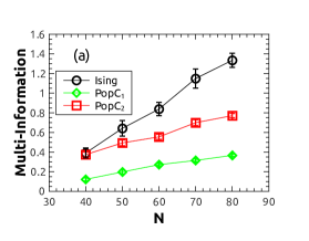
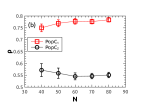
The amount of statistical structure in the neural data due to introducing interactions among neurons can be measured by the multi-information [5]. I first introduce an independent model where only the firing rates of individual neurons are fitted and the corresponding entropy is defined as $S_{{\rm ind}}$. The multi-information is then defined as $I(N)=S_{{\rm ind}}-S_{{\rm model}}$, in which $S_{\rm ind}=\sum_{i}\sum_{x=\pm 1}\mathcal{S}((1+m_{i}x)/2)$, where $\mathcal{S}(u)=-u\ln u$, and $S_{{\rm model}}$ is assumed to be an upper bound to the true entropy. The true entropy for large populations is difficult to estimate since it requires including all possible interactions among neurons. However, the model entropy with low order interaction parameters could be an approximate information capacity for the neural population, which depends on how significant the higher order correlations are in the population.

Fig. 4 (a) shows the multi-information as a function of the network size. ${\rm PopC}_{1}$ and ${\rm PopC}_{2}$ are compared with the Ising model [33], which reconstructs faithfully the pairwise correlations. ${\rm PopC}_{2}$ improves significantly over ${\rm PopC}_{1}$ in capturing the information content of the network, but its multi-information is still below that of the Ising model, which is much more evident for larger network size. This is expected, because only part of third order correlations are captured by ${\rm PopC}_{2}$, while the Ising model describes accurately the entire pairwise correlation profile which may be the main contributor to the collective behavior observed in the population. However, ${\rm PopC}_{2}$ provides us an easy way to understand the higher order correlation, while in the Ising model, it is computationally difficult to estimate the higher order correlations. The average prediction fraction of correlations by ${\rm PopC}_{1}$ and ${\rm PopC}_{2}$ is plotted in Fig. 4 (b). ${\rm PopC}_{1}$ predicts more than $75\%$ of the pairwise correlations, while ${\rm PopC}_{2}$ predicts more than $54\%$ of the triplet correlations. The prediction fraction changes slightly with the network size.

Figure 5: (Color online) Inference performances of ${\rm PopC}_{1}$ on the cortical data ($N=40$, one typical example). (A) Firing rate in the data is reproduced by the model. (B) Two-cell correlations are explained partially by ${\rm PopC}_{1}$ ($99.23\%$). A Monte-Carlo (MC) sampling of the model yields similar results to belief propagation (BP). (C) From the MC samples, three-cell correlations can also be estimated. (D) Probability of $K$ synchronous spiking under the model is compared with that of the data.

Figure 6: (Color online) Inference performances of ${\rm PopC}_{2}$ on the cortical data ($N=40$, one typical example). (A) Firing rate in the data is reproduced by the model. (B) Three-cell correlations are explained partially by ${\rm PopC}_{2}$ ($94.79\%$). (C) Interaction matrix for ${\rm PopC}_{2}$. (D) Probability of $K$ synchronous spiking under the model is compared with that of the data.

III.2 Inference performances on the cortical data

To show the inference performance of both types of population couplings on the cortical data, I randomly select a typical network example of $40$ neurons from the original dataset, and then apply the computation scheme to this typical example. Results are shown in Fig. 5. Surprisingly, the simplified ${\rm PopC}_{1}$ is able to capture as high as $99.23\%$ of pairwise correlations, implying that when a rat performed working memory tasks, there exists a simplified model to describe emergent functional states in the medial prefrontal cortical circuit. Moreover, MC sampling of the ${\rm PopC}_{1}$ model also predicts well the spike synchrony distribution (Fig. 5 (D)). This is very different from that observed in the retinal data. In this sense, the MPC circuit is simple in its functional states when the subject is performing specified tasks.

More interesting circuit features are revealed by ${\rm PopC}_{2}$, which is shown in Fig. 6. About $94.79\%$ of three-cell correlations are explained by ${\rm PopC}_{2}$ in the MPC circuit. The interaction matrix of ${\rm PopC}_{2}$ in Fig. 6 (C) shows a clear non-local structure in the cortical circuit (stripe-like structure). That is, some neurons interact strongly with nearly all the other neurons in the selected population, and these interactions have nearly identical strength of ${\rm PopC}_{2}$. Such neurons having stripe-like structure in the ${\rm PopC}_{2}$ matrix may receive a large number of excitatory inputs from pyramidal neurons [22], and thus play a key role in shaping the collective spiking behavior during the working memory task. The non-local effects are consistent with findings reported in the original experimental paper (cross-correlogram analysis) [22] and the two-neuron interaction map under Ising model (Fig. 7 (a)). Thus, to some extent, ${\rm PopC}_{2}$ may reflect intrinsic connectivity in the cortical circuit, although the relationship between functional connections and anatomical connections has not yet been well established [35]. Lastly, ${\rm PopC}_{2}$ overestimates the tail of the spike synchrony distribution (Fig. 6 (D)), which may be caused by the sampling difficulty of the inferred model (a model with triplet interactions among its elements). The spike synchrony distribution of Ising model is also compared (Fig. 7 (b)).

Figure 7: (Color online) Inference performances of Ising model on the cortical data ($N=40$, one typical example) compared with population coupling. (a) Two-neuron interaction matrix. (b) Probability of $K$ synchronous spiking under the model is compared with that of the data.

Figure 8: (Color online) Multi-information and prediction fraction of correlations under the simplified model for the cortical network. The result is averaged over $10$ network samples for each $N$. (a) Multi-information (in bits) versus the network size $N$. (b) The prediction fraction $\rho$ versus the network size. ${\rm PopC}_{1}$ is used to predict two-cell correlations, and ${\rm PopC}_{2}$ is used to predict three-cell correlations.

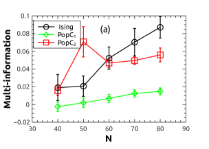
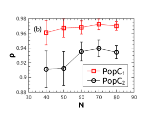
Multi-information versus the cortical network size is plotted in Fig. 8 (a). In the cortical circuit, ${\rm PopC}_{2}$ behaves comparably with the Ising model; even for some network size ($N=50$), it reports a higher information content than the Ising model in the randomly selected subpopulations, which may be caused by the nature of the selected neurons (e.g., inhibitory interneurons [22], and they have stripe-like structure in the ${\rm PopC}_{2}$ matrix). Note that ${\rm PopC}_{1}$ gives an information close to zero for small network sizes, suggesting that by introducing ${\rm PopC}_{1}$, one could not increase significantly the amount of statistical structure in the network activity explained by the model. However, the multi-information of ${\rm PopC}_{1}$ grows with the network size, indicating that the role of ${\rm PopC}_{1}$ would be significant for larger neural populations. Fig. 8 (b) reports the prediction fraction of the correlation profile by applying ${\rm PopC}_{1}$ and ${\rm PopC}_{2}$. Both population couplings can capture over $90\%$ of correlations, which is significantly different from that observed in the retinal data.

IV Discussion

The emergent properties of the neural code arise from interactions among individual neurons. A complete characterization of the population activity is difficult, because on the one hand, the number of potential interactions suffers from a combinatorial explosion, on the other hand, the collective behavior at the network level would become much more complex as the network size grows. In this paper, I develop a theoretical framework to understand how pairwise or higher order correlations arise and the basic circuit variables corresponding to these correlation structures. The model is based on the concept of population coupling, characterizing the relationship between local firing activity of individual neuron or neuron-pair and the global neural activity. An advantage is that, it provides a low dimensional and neurobiologically interpretable representation to understand the functional interaction between neurons and their correlation structures. In particular, the concept of population coupling and the associated mean field method used in this paper offer an easy way to evaluate higher order correlations, while the usual sampling method is computationally hard and traditional models (e.g., Ising model) lack a direct interpretation of higher order correlations in terms of simplified (population) couplings.

With the mean field method, the concept of population coupling is tested on two different types of neural data. One is the firing neural activities of retinal ganglion cells under natural movie stimuli. The other is the population activities of medial prefrontal cortex when a rat was performing odor-place matching working memory tasks.

For the retinal data, on average ${\rm PopC}_{1}$ accounts for more than $75\%$ of pairwise correlations, and ${\rm PopC}_{2}$ accounts for over $54\%$ of three-cell correlations. The interaction matrix of ${\rm PopC}_{2}$ contains information about the functional interaction features in the retinal circuitry. It seems that a retinal neuron can be paired with not only negatively strong couplings, but also slightly positive couplings. Only a few pairs of neurons have strong correlations with the global activity of the population. To describe the spike synchrony distribution, ${\rm PopC}_{2}$ performs better than ${\rm PopC}_{1}$, nevertheless, both of them could not capture the trend of the tail (rare events related to higher order interactions existing in the network). This is not surprising, because ${\rm PopC}_{1}$ and ${\rm PopC}_{2}$ are simplified descriptions of the original high dimensional neural activity, taking the trade-off between the computation complexity and the description goodness.

To extract the statistical structure embedded in the neural population, ${\rm PopC}_{2}$ improves significantly over ${\rm PopC}_{1}$, and has further additional benefit of describing the third-order correlations observed in the data, as ${\rm PopC}_{2}$ could be used to construct triplet interactions among neurons, although direct constructing all possible triplet interactions is extremely computationally difficult.

Unlike the retinal circuit, the cortical circuit yields a much smaller absolute value of the multi-information, implying that no significant higher order correlations (interactions) were present in the neural circuit when the circuit was carrying out task-related information processing rather than encoding well-structured stimuli (as in the retinal network). This also explains why a simplified description such as ${\rm PopC}_{1}$ and ${\rm PopC}_{2}$ is accurate enough to capture the main features of the population activity, including the spike synchrony distribution. The inferred model on the cortical data reveals a different interaction map from that of the retinal circuit. In the cortical circuit, neurons form the stripe-like structure in the interaction matrix, suggesting that these neurons may receive a large number of excitatory inputs [22]. These inputs may come from different layers of cortex, and they can execute top-down or bottom-up information processing, thus modulate the global brain state in the target cortex during behavioral tasks.

Before summary of this work, I made some discussions about two relevant recent studies on population coupling (see notes added). Ref. [32] modeled directly the joint probability distribution of individual neural response and population rate (the number of neurons simultaneously active) by linear coupling and complete coupling models. The linear coupling reproduces separately the distribution of individual neuronal state and the population rate distribution, and their couplings, while ${\rm PopC}_{1}$ introduced in my work reproduces mean firing rate and the correlation between individual neuronal state and the background population activity (except the neuron itself). Note that ${\rm PopC}_{1}$ does not model population rate distribution explicitly, which is hard to interpret in terms of functional connectivity. The complete-coupling model reproduces the joint probability distributions between the response of each neuron and the population rate, from which it is hard to conclude that the high-order interactions responsible for high-order correlations can be interpreted and tested. However, ${\rm PopC}_{2}$ reproduces mean firing rate and the correlation between neuron-pair activities and the background population activity (except the neuron-pair itself), and thus explains high-order correlations by an energy model. Furthermore, in this sense, this work overcame a weakness pointed out in another independent later work of population coupling [36], which fitted directly the population rate distribution and the firing probability for each neuron conditioned on the population rate, and analogously the corresponding model parameters can not be readily interpretable in a biological setting. Due to intrinsic difference in model definitions, these two relevant works have nice properties of studying tuning curves of individual neurons to the population rate, and sampling from the model to reproduce the population synchrony distribution.

In summary, I develop a theoretical model of population coupling and its advanced form, to relate the correlation profile in the neural collective activity to the basic circuit variables. The practical dimensional reduction method is tested on different types of neural data, and specific features of neural circuit are revealed. This model aiming at describing high order correlations with a low order representation, is expected to be useful for modeling big neural data. Note that the interaction matrices shown in Fig. 2 and Fig. 6 are qualitatively robust to changes of the data size to only the first half (data not shown), verifying that the revealed features are not an artifact of overfitting. However, it still deserves further studies by introducing regularization in the learning equation. It is also very interesting to incorporate more physiologically plausible parameters to explain how the collective spiking behavior arises from the microscopic interactions among the basic units. Another interesting study is to clarify the role of higher order correlations in decoding performances based on maximum likelihood principles [37, 38].

note added.—After I submitted this work to arXiv:1602.08299, I became aware of Ref. [32] (arXiv:1606.08889), and later Ref. [36] (bioRxiv, 2016). Discussions about these two recent relevant works are made in the last section of this paper.

Appendix A Derivation of mean-field equations

In this appendix, I give a simple derivation of mean-field equations given in Sec. II. More details can be obtained from Refs [30, 31]. First, after removing an interaction $a$, one defines the cavity probability $P_{i\rightarrow a}(s_{i})=\frac{e^{h_{i}s_{i}}}{Z_{i}}\prod_{b\in\partial i\backslash a}\hat{P}_{b\rightarrow i}(s_{i})$, where the product comes from the physical meaning of the second kind of cavity probability, namely $\hat{P}_{b\rightarrow i}(s_{i})$ defined as the cavity probability when only the connection from $b$ to $i$ is retained while other neighbors of $i$ are removed (so-called cavity probability). $\hat{P}_{b\rightarrow i}(s_{i})$ is thus formulated as $\sum_{s_{j}:j\in\partial b\backslash i}e^{\Gamma_{b}\prod_{j\in\partial b}s_{j}}\prod_{j\in\partial b\backslash i}P_{j\rightarrow b}(s_{j})$. With these two probabilities, it follows that the cavity magnetization $m_{i\rightarrow a}=\sum_{s_{i}}s_{i}P_{i\rightarrow a}(s_{i})=\tanh\left(h_{i}+\sum_{b\in\partial i\backslash a}u_{b\rightarrow i}\right)$, where $u_{b\rightarrow i}$ is named cavity bias in physics [29]. It is related to $\hat{m}_{b\rightarrow i}$ by $\hat{m}_{b\rightarrow i}=\tanh(u_{b\rightarrow i})=\sum_{s_{i}}s_{i}\hat{P}_{b\rightarrow i}(s_{i})$.

More specifically, the cavity magnetization is derived as follows,

$$\begin{split}m_{i\rightarrow a}&=P_{i\rightarrow a}(+1)-P_{i\rightarrow a}(-1)=\frac{e^{h_{i}}\prod_{b\in\partial i\backslash a}\hat{P}_{b\rightarrow i}(+1)-e^{-h_{i}}\prod_{b\in\partial i\backslash a}\hat{P}_{b\rightarrow i}(-1)}{e^{h_{i}}\prod_{b\in\partial i\backslash a}\hat{P}_{b\rightarrow i}(+1)+e^{-h_{i}}\prod_{b\in\partial i\backslash a}\hat{P}_{b\rightarrow i}(-1)}\\ &=\frac{e^{h_{i}}-e^{-h_{i}-2\sum_{b\in\partial i\backslash a}u_{b\rightarrow i}}}{e^{h_{i}}+e^{-h_{i}-2\sum_{b\in\partial i\backslash a}u_{b\rightarrow i}}}\\ &=\tanh\left(h_{i}+\sum_{b\in\partial i\backslash a}u_{b\rightarrow i}\right),\end{split}$$ (10a)

where I have used the definition $u_{b\rightarrow i}\equiv\frac{1}{2}\ln\frac{\hat{P}_{b\rightarrow i}(+1)}{\hat{P}_{b\rightarrow i}(-1)}$. Next, I show how to derive the cavity bias. First, for pairwise interaction,

$$\begin{split}u_{b\rightarrow i}&=\frac{1}{2}\ln\frac{e^{\Gamma_{b}}P_{j\rightarrow b}(+1)+e^{-\Gamma_{b}}P_{j\rightarrow b}(-1)}{e^{-\Gamma_{b}}P_{j\rightarrow b}(+1)+e^{\Gamma_{b}}P_{j\rightarrow b}(-1)}\\ &=\frac{1}{2}\ln\frac{1+\tanh\Gamma_{b}m_{j\rightarrow b}}{1-\tanh\Gamma_{b}m_{j\rightarrow b}}\\ &=\tanh^{-1}\left(\tanh\Gamma_{b}m_{j\rightarrow b}\right),\end{split}$$ (11a)

where I have used the parameterization $P_{j\rightarrow b}(s_{j})=\frac{1+s_{j}m_{j\rightarrow b}}{2}$, and the mathematical identity $e^{2z}=\frac{1+\tanh z}{1-\tanh z}$. Similarly, for triplet interaction,

$$\begin{split}u_{b\rightarrow i}&=\frac{1}{2}\ln\frac{e^{\Gamma_{b}}[P_{j\rightarrow b}(+1)P_{k\rightarrow b}(+1)+P_{j\rightarrow b}(-1)P_{k\rightarrow b}(-1)]+e^{-\Gamma_{b}}[P_{j\rightarrow b}(+1)P_{k\rightarrow b}(-1)+P_{j\rightarrow b}(-1)P_{k\rightarrow b}(+1)]}{e^{-\Gamma_{b}}[P_{j\rightarrow b}(+1)P_{k\rightarrow b}(+1)+P_{j\rightarrow b}(-1)P_{k\rightarrow b}(-1)]+e^{\Gamma_{b}}[P_{j\rightarrow b}(+1)P_{k\rightarrow b}(-1)+P_{j\rightarrow b}(-1)P_{k\rightarrow b}(+1)]}\\ &=\frac{1}{2}\ln\frac{1+e^{-2\Gamma_{b}}\frac{1-m_{j\rightarrow b}m_{k\rightarrow b}}{1+m_{j\rightarrow b}m_{k\rightarrow b}}}{e^{-2\Gamma_{b}}+\frac{1-m_{j\rightarrow b}m_{k\rightarrow b}}{1+m_{j\rightarrow b}m_{k\rightarrow b}}}\\ &=\tanh^{-1}\left(\tanh\Gamma_{b}m_{j\rightarrow b}m_{k\rightarrow b}\right).\end{split}$$ (12a)

These results are written in a compact form as Eq. (6) in the main text.

Similarly, the single neuron magnetization $m_{i}$ is obtained via $m_{i}=\frac{1}{Z_{i}}\sum_{s_{i}}s_{i}e^{h_{i}s_{i}}\prod_{b\in\partial i}\hat{P}_{b\rightarrow i}(s_{i})$, where $Z_{i}$ is a normalization constant, and the multi-neuron correlation $C_{a}=\frac{1}{Z_{a}}\sum_{s_{i}:i\in\partial a}\prod_{i\in\partial a}s_{i}e^{\Gamma_{a}\prod_{i\in\partial a}s_{i}}\prod_{i\in\partial a}P_{i\rightarrow a}(s_{i})$, where $Z_{a}$ is a normalization constant. Note that $Z_{i}$ and $Z_{a}$ are also related to the free energy contribution of single neuron and neuronal interaction [30], respectively. The full (non-cavity) magnetization can be derived in a similar manner to Eq. (10), as $m_{i}=\tanh\left(h_{i}+\sum_{b\in\partial i}u_{b\rightarrow i}\right)$. In detail, the two-point correlation $C_{a}$ ($|\partial a|=2$) is computed as follows,

$$\begin{split}C_{a}&\equiv\left<s_{i}s_{j}\right>=\frac{\sum_{s_{i},s_{j}}s_{i}s_{j}e^{\Gamma_{a}s_{i}s_{j}}P_{i\rightarrow a}(s_{i})P_{j\rightarrow a}(s_{j})}{\sum_{s_{i},s_{j}}e^{\Gamma_{a}s_{i}s_{j}}P_{i\rightarrow a}(s_{i})P_{j\rightarrow a}(s_{j})}\\ &=\frac{e^{2\Gamma_{a}}-\frac{1-m_{j\rightarrow a}m_{i\rightarrow a}}{1+m_{j\rightarrow a}m_{i\rightarrow a}}}{e^{2\Gamma_{a}}+\frac{1-m_{j\rightarrow a}m_{i\rightarrow a}}{1+m_{j\rightarrow a}m_{i\rightarrow a}}}\\ &=\frac{\tanh\Gamma_{a}+m_{i\rightarrow a}m_{j\rightarrow a}}{1+\tanh\Gamma_{a}m_{i\rightarrow a}m_{j\rightarrow a}}.\end{split}$$ (13a)

Analogously, three-point correlation ($|\partial a|=3$) can be evaluated as

$$\begin{split}C_{a}&\equiv\left<s_{i}s_{j}s_{k}\right>=\frac{\sum_{s_{i},s_{j},s_{k}}s_{i}s_{j}s_{k}e^{\Gamma_{a}s_{i}s_{j}s_{k}}P_{i\rightarrow a}(s_{i})P_{j\rightarrow a}(s_{j})P_{k\rightarrow a}(s_{k})}{\sum_{s_{i},s_{j},s_{k}}e^{\Gamma_{a}s_{i}s_{j}s_{k}}P_{i\rightarrow a}(s_{i})P_{j\rightarrow a}(s_{j})P_{k\rightarrow a}(s_{k})}\\ &=\frac{e^{2\Gamma_{a}}-\frac{1-m_{j\rightarrow a}m_{i\rightarrow a}m_{k\rightarrow a}}{1+m_{j\rightarrow a}m_{i\rightarrow a}m_{k\rightarrow a}}}{e^{2\Gamma_{a}}+\frac{1-m_{j\rightarrow a}m_{i\rightarrow a}m_{k\rightarrow a}}{1+m_{j\rightarrow a}m_{i\rightarrow a}m_{k\rightarrow a}}}\\ &=\frac{\tanh\Gamma_{a}+m_{i\rightarrow a}m_{j\rightarrow a}m_{k\rightarrow a}}{1+\tanh\Gamma_{a}m_{i\rightarrow a}m_{j\rightarrow a}m_{k\rightarrow a}}.\end{split}$$ (14a)

These results are written in a compact form as Eq. (8b) in the main text.

Finally, the partition function $Z_{i}$ for pairwise interaction is computed as follows,

$$\begin{split}Z_{i}&=e^{h_{i}}\prod_{b\in\partial i}\hat{P}_{b\rightarrow i}(+1)+e^{-h_{i}}\prod_{b\in\partial i}\hat{P}_{b\rightarrow i}(-1)\\ &=e^{h_{i}}\prod_{b\in\partial i}\cosh\Gamma_{b}(1+\tanh\Gamma_{b}m_{j\rightarrow b})+e^{-h_{i}}\prod_{b\in\partial i}\cosh\Gamma_{b}(1-\tanh\Gamma_{b}m_{j\rightarrow b}),\end{split}$$ (15a)

where I have used $\hat{P}_{b\rightarrow i}(s_{i})=e^{\Gamma_{b}s_{i}}P_{j\rightarrow b}(+1)+e^{-\Gamma_{b}s_{i}}P_{j\rightarrow b}(-1)$ and the magnetization parameterization of $P_{j\rightarrow b}$. For triplet interaction, $\hat{P}_{b\rightarrow i}(s_{i})=e^{\Gamma_{b}s_{i}}[P_{j\rightarrow b}(+1)P_{k\rightarrow b}(+1)+P_{j\rightarrow b}(-1)P_{k\rightarrow b}(-1)]+e^{-\Gamma_{b}s_{i}}[P_{j\rightarrow b}(+1)P_{k\rightarrow b}(-1)+P_{j\rightarrow b}(-1)P_{k\rightarrow b}(+1)]$, and the corresponding $Z_{i}=e^{h_{i}}\prod_{b\in\partial i}\cosh\Gamma_{b}(1+\tanh\Gamma_{b}m_{j\rightarrow b}m_{k\rightarrow b})+e^{-h_{i}}\prod_{b\in\partial i}\cosh\Gamma_{b}(1-\tanh\Gamma_{b}m_{j\rightarrow b}m_{k\rightarrow b})$. Following the same line, the partition function $Z_{a}$ is evaluated for pairwise interaction as

$$\begin{split}Z_{a}&=\sum_{s_{i},s_{j}}e^{\Gamma_{a}s_{i}s_{j}}P_{i\rightarrow a}(s_{i})P_{j\rightarrow a}(s_{j})\\ &=\cosh\Gamma_{a}[1+\tanh\Gamma_{a}m_{i\rightarrow a}m_{j\rightarrow a}].\end{split}$$ (16a)

Similarly, the partition function $Z_{a}$ for triplet interaction can be computed as

$$\begin{split}Z_{a}&=\sum_{s_{i},s_{j},s_{k}}e^{\Gamma_{a}s_{i}s_{j}s_{k}}P_{i\rightarrow a}(s_{i})P_{j\rightarrow a}(s_{j})P_{k\rightarrow a}(s_{k})\\ &=\cosh\Gamma_{a}[1+\tanh\Gamma_{a}m_{i\rightarrow a}m_{j\rightarrow a}m_{k\rightarrow a}],\end{split}$$ (17a)

which is exactly the compact equation given in the main text.

References

- [1] R. Q. Quiroga and S. Panzeri. Extracting information from neuronal populations: information theory and decoding approaches. Nat Rev Neurosci, 10:173, 2009.
- [2] R. Yuste. From the neuron doctrine to neural networks. Nat Rev Neurosci, 16:487, 2015.
- [3] I. H. Stevenson and K. P. Kording. How advances in neural recording affect data analysis. Nat Rev Neurosci, 14:139, 2011.
- [4] M. R. Cohen and A. Kohn. Measuring and interpreting neuronal correlations. Nat Neurosci, 14:811, 2011.
- [5] E. Schneidman, M. J. Berry, R. Segev, and W. Bialek. Weak pairwise correlations imply strongly correlated network states in a neural population. Nature, 440:1007, 2006.
- [6] S. Cocco, S. Leibler, and R. Monasson. Neuronal couplings between retinal ganglion cells inferred by efficient inverse statistical physics methods. Proc. Natl. Acad. Sci. USA, 106:14058, 2009.
- [7] J. H. Macke, M. Opper, and M. Bethge. Common input explains higher-order correlations and entropy in a simple model of neural population activity. Phys. Rev. Lett, 106:208102, 2011.
- [8] Elad Ganmor, Ronen Segev, and Elad Schneidman. The architecture of functional interaction networks in the retina. The Journal of Neuroscience, 31:3044, 2011.
- [9] L. Martignon, G. Deco, K. Laskey, M. Diamond, W. Freiwald, and E. Vaadia. Neural coding: higher-order temporal patterns in the neurostatistics of cell assemblies. Neural Computation, 12:2621, 2000.
- [10] M. J. Schnitzer and M. Meister. Multineuronal firing patterns in the signal from eye to brain. Neuron, 37:499, 2003.
- [11] I. E. Ohiorhenuan, F. Mechler, K. P. Purpura, A. M. Schmid, Q. Hu, and J. D. Victor. Sparse coding and high-order correlations in fine-scale cortical networks. Nature, 466:617, 2010.
- [12] S.-I. Amari, H. Nakahara, S. Wu, and Y. Sakai. Synchronous firing and higher-order interactions in neuron pool. Neural Computation, 15:127, 2003.
- [13] F. Montani, E. Phoka, M. Portesi, and S. R. Schultz. Statistical modelling of higher-order correlations in pools of neural activity. Physica A: Statistical Mechanics and its Applications, 392:3066, 2013.
- [14] E. Ganmor, R. Segev, and E. Schneidman. Sparse low-order interaction network underlies a highly correlated and learnable neural population code. Proc. Natl. Acad. Sci. USA, 108:9679, 2011.
- [15] Shan Yu, Hongdian Yang, Hiroyuki Nakahara, Gustavo S. Santos, Danko Nikolić, and Dietmar Plenz. Higher-order interactions characterized in cortical activity. The Journal of Neuroscience, 31:17514, 2011.
- [16] G. Tkacik, O. Marre, T. Mora, D. Amodei, M. J. Berry II, and W. Bialek. The simplest maximum entropy model for collective behavior in a neural network. Journal of Statistical Mechanics: Theory and Experiment, 2013:P03011, 2013.
- [17] G. Tkacik, O. Marre, D. Amodei, E. Schneidman, W. Bialek, and M. J. Berry II. Searching for collective behavior in a large network of sensory neurons. PLoS Comput Biol, 10:e1003408, 2014.
- [18] U. Köster, J. Sohl-Dickstein, C. M. Gray, and B. A. Olshausen. Modeling higher-order correlations within cortical microcolumns. PLoS Comput Biol, 10:e1003684, 2014.
- [19] Haiping Huang. Effects of hidden nodes on network structure inference. Journal of Physics A: Mathematical and Theoretical, 48:355002, 2015.
- [20] H. Shimazaki, K. Sadeghi, T. Ishikawa, Y. Ikegaya, and T. Toyoizumi. Simultaneous silence organizes structured higher-order interactions in neural populations. Scientific Reports, 5:9821, 2015.
- [21] M. Okun, N. A. Steinmetz, L. Cossell, M. F. Iacaruso, H. Ko, P. Bartho, T. Moore, S. B. Hofer, T. D. Mrsic-Flogel, M. Carandini, and K. D. Harris. Diverse coupling of neurons to populations in sensory cortex. Nature, 521:511, 2015.
- [22] S. Fujisawa, A. Amarasingham, M. T. Harrison, and G. Buzsaki. Behavior-dependent short-term assembly dynamics in the medial prefrontal cortex. Nat Neurosci, 11:823, 2008.
- [23] Rob R. de Ruyter van Steveninck, Geoffrey D. Lewen, Steven P. Strong, Roland Koberle, and William Bialek. Reproducibility and variability in neural spike trains. Science, 275:1805, 1997.
- [24] Michael Okun, Pierre Yger, Stephan L Marguet, Florian Gerard-Mercier, Andrea Benucci, Steffen Katzner, Laura Busse, Matteo Carandini, and Kenneth D Harris. Population rate dynamics and multineuron firing patterns in sensory cortex. The Journal of Neuroscience, 32:17108, 2012.
- [25] Simona Cocco and Rémi Monasson. Adaptive cluster expansion for the inverse ising problem: convergence, algorithm and tests. J. Stat. Phys, 147:252, 2012.
- [26] H. Huang. Sparse hopfield network reconstruction with regularization. Eur. Phys. J. B, 86:484, 2013.
- [27] Y. Roudi, E. Aurell, and J. Hertz. Statistical physics of pairwise probability models. Front. Comput. Neurosci, 3:1, 2009.
- [28] Haiping Huang and Taro Toyoizumi. Clustering of neural code words revealed by a first-order phase transition. Phys. Rev. E, 93:062416, 2016.
- [29] M. Mézard and G. Parisi. The bethe lattice spin glass revisited. Eur. Phys. J. B, 20:217, 2001.
- [30] H. Huang and H. Zhou. Cavity approach to the sourlas code system. Phys. Rev. E, 80:056113, 2009.
- [31] M. Mézard and A. Montanari. Information, Physics, and Computation. Oxford University Press, Oxford, 2009.
- [32] Christophe Gardella, Olivier Marre, and Thierry Mora. A Tractable Method for Describing Complex Couplings between Neurons and Population Rate. eneuro, 3:e0160–15.2016, 2016. arXiv:1606.08889.
- [33] H. Huang and H. Zhou. Counting solutions from finite samplings. Phys. Rev. E, 85:026118, 2012.
- [34] Ko Ho, Hofer Sonja B., Pichler Bruno, Buchanan Katherine A., Sjostrom P. Jesper, and Mrsic-Flogel Thomas D. Functional specificity of local synaptic connections in neocortical networks. Nature, 473:87, 2011.
- [35] Dimitri Yatsenko, Josic Kresimir, Ecker Alexander S., Froudarakis Emmanouil, Cotton R. James, and Tolias Andreas S. Improved Estimation and Interpretation of Correlations in Neural Circuits. PLoS Comput Biol, 11:e1004083, 2015.
- [36] Cian O’Donnell, J Tiago Goncalves, Nick Whiteley, Carlos Portera-Cailliau, and Terrence J Sejnowski. The population tracking model: A simple, scalable statistical model for neural population data. Neural Computation, 29:50–93, 2017.
- [37] Michael T. Schaub and Simon R. Schultz. The ising decoder: reading out the activity of large neural ensembles. J Comput Neurosci, 32:101, 2012.
- [38] Greg Schwartz, Jakob Macke, Dario Amodei, Hanlin Tang, and Michael J. Berry. Low error discrimination using a correlated population code. J Neurophysiol, 108:1069, 2012.