Multiple testing of local maxima
for detection of peaks on the (celestial) sphere

Dan Cheng Division of Biostatistics, University of California, San Diego Valentina Cammarota Department of Mathematics, University of Rome Tor Vergata Yabebal Fantaye Department of Mathematics, University of Rome Tor Vergata Domenico Marinucci Department of Mathematics, University of Rome Tor Vergata Armin Schwartzman Division of Biostatistics, University of California, San Diego
Abstract

We present a topological multiple testing scheme for detecting peaks on the sphere under isotropic Gaussian noise, where tests are performed at local maxima of the observed field filtered by the spherical needlet transform. Our setting is different from the standard Euclidean/large same asymptotic framework, yet highly relevant to realistic experimental circumstances for some important areas of application in astronomy. More precisely, we focus on cases where a single realization of a smooth isotropic Gaussian random field on the sphere is observed, and a number of well-localized signals are superimposed on such background field. The proposed algorithms, combined with the Benjamini-Hochberg procedure for thresholding p-values, provide asymptotic strong control of the False Discovery Rate (FDR) and power consistency as the signal strength and the frequency of the needlet transform get large. This novel multiple testing method is illustrated in a simulation of point-source detection in Cosmic Microwave Background radiation (CMB) data.

  • β€’

    Keywords and Phrases: Gaussian random fields; Sphere; CMB; Height distribution; Overshoot distribution; Needlet transform; P-value; Threshold; False discovery rate; Power.

  • β€’

    AMS Classification: 60G15; 60G60; 62H15; 62M15; 62M40

1 Introduction

A classical problem of modern high-dimensional statistics is multiple testing in the presence of background noise. Applications are common in the areas of neuroimaging, genomic arrays and astronomy. These issues become particularly challenging when the background noise is allowed to exhibit more realistic properties than the simple i.i.d.formulae-sequence𝑖𝑖𝑑i.i.d. framework, in particular when noise is modeled as a stochastic process or a random field. In this setting, important progresses have been recently obtained combining ideas from two different streams of research, namely techniques from the multiple testing literature, such as False Discovery Rate (FDR) algorithms, and techniques to investigate excursion probabilities and local maxima for random fields; we refer for instance to [1, 43, 9, 10] for further background and discussion. These works have covered applications in a univariate and multivariate Euclidean setting; analytic properties have been derived under a large sample asymptotic framework, i.e., under the assumption that the domain of observations is growing steadily, together with the signals to be detected.

In this paper we introduce a related multiple testing procedure in a setting that is different from the standard Euclidean/large same asymptotic framework, yet highly relevant to realistic experimental circumstances for some important areas of application in astronomy. More precisely, we shall focus on cases where a single realization of a smooth isotropic Gaussian random field on the sphere is observed, and a number of well-localized signals are superimposed on such background field. This is exactly the setting for the so-called point-source detection issue in Cosmic Microwave Background radiation (CMB) data experiments (see i.e., [33, 35, 34, 37]). As discussed now in any modern textbook in Cosmology (see for instance [13, 15]), CMB data can be viewed as a single realization of an isotropic Gaussian random field, which represents a β€œsnapshot” of the Universe at the last scattering surface, i.e. the time (approximately 4Γ—1054superscript1054\times 10^{5} years after the Big Bang, or 1.38Γ—10101.38superscript10101.38\times 10^{10} years ago) when photons decoupled from electrons and protons and started to travel nearly without interactions in space. As such, CMB has been repeatedly defined as a goldmine of information on Cosmology - two very successful satellite experiments (WMAP from NASA, see http://map.gsfc.nasa.gov/ and Planck from ESA, see http://www.esa.int/Our_Activities/Space_Science/Planck) have now produced full-sky maps of CMB radiations, and these data have been used in several thousand papers over the last few years to address a number of fundamental questions on the dynamics of the Big Bang, the matter-energy content of the Universe, the mechanisms of structure formation, and several others.

From the experimental point of view, it is very important to recall that, superimposed Β to CMB radiation, a number of foreground β€œcontaminants” are present; as a first approximation, we can view them as point-like objects (galaxies or clusters of galaxies, typically). A major statistical challenge in the analysis of CMB data is the proper identification of such sources; on the one hand this is important for the proper construction of filtered CMB maps, on the other hand these sources are of great interest on their own as proper astrophysical objects (in some cases they can be matched with existing catalogues, while in other cases they lead to new discoveries). A number of algorithms have been proposed for these tasks, see for instance [2, 3, 25, 41, 42]. These solutions have all been shown to perform well in practice; however, they have all avoided to face the specific challenges of multiple testing, and in particular none of them has been shown to control in any proper statistical way any aggregate statistics such as the classical Family-Wise Error Rate (FWER), False Discovery Proportion (FDP) or False Discovery Rate (FDR).

Our purpose in this paper is to develop in such a spherical framework a rigorous statistical procedure to control error rates in a multiple testing framework. Our starting idea is to extend to these circumstances the Smoothing and TEsting of Maxima (STEM) algorithm advocated in [43, 10], and investigate rigorously its statistical properties. While our construction follows in several ways what was earlier done by these authors, we wish to stress that the new spherical framework poses some major technical and foundational new challenges.

The first of these new challenges is the proper definition of filters and point-like signals in a spherical framework. Here, natural solutions can be found by exploiting recent developments in the analysis of spherical random fields an spherical wavelets. In particular, we can define bell-shaped signals by adopting a natural definition of a Gaussian distribution on the sphere, motivated in terms of diffusion processes; likewise, filtering can be implemented by wavelet techniques - we find particularly convenient the Mexican needlet construction introduced by [16, 17], see also [40] for some earlier applications to CMB data.

A second, more delicate, issue is the rigorous investigation of asymptotic statistical properties. A crucial staple of the STEM algorithm is the possibility to control the FDR, assuming convergence of the empirical distribution of the maxima to its theoretical counterpart. In standard settings this can be done by resorting to ergodicity properties in a β€œlarge sample asymptotics” framework, i.e. assuming that the domain of the observations grows larger and larger. This form of ergodic properties cannot be exploited here because our spherical domain is compact. We shall hence require a convergence result on the empirical distribution of maxima in a high-frequency/fixed domain setting: this result extends to the case of the needlet transform some related computations which were recently performed in [8] for the case of random spherical harmonics. In this sense, our setting is related to the increasingly popular fixed-domain asymptotics approach for the analysis of random fields, see i.e., [23, 24].

The plan of this paper is as follows. Our basic setting and model is introduced in Section 2, with Section 3 devoted to a careful discussion on the nature and effects of filtering. Section 4 provides a description of the multiple testing scheme and discusses the error and power definitions, including the derivation of asymptotic p𝑝p-values and our adoption of Benjamini and Hochberg’s (1995) pioneering approach [6]. The proofs of FDR control and tests consistency are collected in Section 5, while in Section 6 we provide some numerical results on the empirical performance of the proposed procedures in simulated CMB fields. Finally, two (long) Appendixes provide a large part of the proofs, in particular, the details of the high frequency ergodicity of the empirical distribution function of local maxima.

For clarity of exposition and concreteness of motivations, throughout the paper we mainly justify our framework resorting to applications in a Cosmological framework; it is to be stressed, however, that our approach may be applied to many other experimental contexts where data are collected on a sphere, such as Geophysics, Atmospheric Sciences, Solar Physics, and even (with some approximations) Neuroimaging, to mention only a few.

1.1 Acknowledgements

This research was supported by the ERC Grant n.277742 Pascal (PI Domenico Marinucci); we are grateful to Igor Wigman for many insights and suggestions on the computation of variances of critical points. Corresponding author: Valentina Cammarota, Department of Mathematics, University of Rome Tor Vergata, via della Ricerca Scientifica, 1, I-00133, Italy, cammarot@mat.uniroma2.it.

2 The model

The purpose of this Section is to introduce our model in detail. As motivated above, our purpose here is to represent a situation where a large number of β€œpoint sources” is superimposed on some isotropic background β€œnoise”. Of course, the notions of β€œnoise” and β€œsignal”, here as in any other motivating field, is very much conventional. For instance, in the CMB-related applications that we have in mind the background Gaussian field is eventually the primary object of physical interest for many (most) researchers, while the super-imposed point sources are contaminants to be removed; in other astrophysical areas, on the contrary, the identification of the sources may be by itself a major scientific goal (a very recent catalogue of detected point sources/astrophysical objects is given for instance by [37]).

2.1 Signal model

To introduce our model for the signal, we first need to justify the notion of a β€œGaussian-shaped” density on the sphere. We do this in terms of the diffusion equation on the sphere. More formally, let π•Š2superscriptπ•Š2{\mathbb{S}}^{2} denote the unit sphere in ℝ3superscriptℝ3\mathbb{R}^{3}. The diffusion equation on the sphere is then given by

βˆ‚βˆ‚t​h​(x;t,x0)π‘‘β„Žπ‘₯𝑑subscriptπ‘₯0\displaystyle\frac{\partial}{\partial t}h(x;t,x_{0}) =βˆ’Ξ”S2​ ​h​(x;t,x0)absentsubscriptΞ”superscript𝑆2Β β„Žπ‘₯𝑑subscriptπ‘₯0\displaystyle=-\Delta_{S^{2}\text{ }}h(x;t,x_{0})
h​(x;0,x0)β„Žπ‘₯0subscriptπ‘₯0\displaystyle h(x;0,x_{0}) =Ξ΄x0​(x),absentsubscript𝛿subscriptπ‘₯0π‘₯\displaystyle=\delta_{x_{0}}(x),

where Ξ”S2​ subscriptΞ”superscript𝑆2Β \Delta_{S^{2}\text{ }} is the Laplacian operator in π•Š2superscriptπ•Š2{\mathbb{S}}^{2} and Ξ΄x0​(x)subscript𝛿subscriptπ‘₯0π‘₯\delta_{x_{0}}(x) identifies formally a Dirac’s delta function centered at x0∈S2subscriptπ‘₯0superscript𝑆2x_{0}\in S^{2}. It is standard to write the solution in terms of diffusion operators as

h​(x;t,x0)=exp⁑(βˆ’t​ΔS2​ )​h​(x;0,x0)=βˆ‘β„“2​ℓ+14​π​exp⁑(βˆ’t​λℓ)​Pℓ​(⟨x0,x⟩)​,Β β„Žπ‘₯𝑑subscriptπ‘₯0𝑑subscriptΞ”superscript𝑆2Β β„Žπ‘₯0subscriptπ‘₯0subscriptβ„“2β„“14πœ‹π‘‘subscriptπœ†β„“subscript𝑃ℓsubscriptπ‘₯0π‘₯,Β h(x;t,x_{0})=\exp(-t\Delta_{S^{2}\text{ }})h(x;0,x_{0})=\sum_{\ell}\frac{2\ell+1}{4\pi}\exp(-t\lambda_{\ell})P_{\ell}(\left\langle x_{0},x\right\rangle)\text{, }

where Ξ»β„“:=ℓ​(β„“+1)assignsubscriptπœ†β„“β„“β„“1\lambda_{\ell}:=\ell(\ell+1) denotes the set of eigenvalues of the spherical Laplacian, β„“=1,2,…,β„“12…\ell=1,2,..., while {Pℓ​(β‹…)}subscript𝑃ℓ⋅\left\{P_{\ell}(\cdot)\right\} represents the family of Legendre polynomials

Pℓ​(u)=(βˆ’1)β„“2ℓ​dβ„“d​uℓ​(1βˆ’u2)β„“,β„“=1,2,3,…formulae-sequencesubscript𝑃ℓ𝑒superscript1β„“superscript2β„“superscript𝑑ℓ𝑑superscript𝑒ℓsuperscript1superscript𝑒2β„“β„“123…P_{\ell}(u)=\frac{(-1)^{\ell}}{2^{\ell}}\frac{d^{\ell}}{du^{\ell}}(1-u^{2})^{\ell},\qquad\ell=1,2,3,\ldots

i.e., P1​(u)=usubscript𝑃1𝑒𝑒P_{1}(u)=u, P2​(u)=(3​u2βˆ’1)/2subscript𝑃2𝑒3superscript𝑒212P_{2}(u)=(3u^{2}-1)/2, P3​(u)=(5​u3βˆ’3​u)/2subscript𝑃3𝑒5superscript𝑒33𝑒2P_{3}(u)=(5u^{3}-3u)/2, etc., and βŸ¨β‹…,β‹…βŸ©β‹…β‹…\left\langle\cdot,\cdot\right\rangle denotes inner product on π•Š2.superscriptπ•Š2{\mathbb{S}}^{2}. By a straightforward analogy with the Euclidean case, it is natural/customary to view ux0​(β‹…,t)subscript𝑒subscriptπ‘₯0⋅𝑑u_{x_{0}}(\cdot,t) as the density on π•Š2superscriptπ•Š2{\mathbb{S}}^{2} of a β€œspherical Gaussian” centred on x0subscriptπ‘₯0x_{0} and having variance t𝑑t.

Our β€œpoint source” signal will be built from a set of such bell-shaped distributions, localized on some family of points ΞΎksubscriptπœ‰π‘˜\xi_{k}, k=1,…,Nπ‘˜1…𝑁k=1,\ldots,N, belonging to π•Š2superscriptπ•Š2{\mathbb{S}}^{2}; we shall allow later their number to grow (N=N​(j)β†’βˆžπ‘π‘π‘—β†’N=N(j)\rightarrow\infty as jβ†’βˆžβ†’π‘—j\rightarrow\infty, where j𝑗j is the frequency), and their shape to become more and more localized (t=tN​(j)β†’0𝑑subscript𝑑𝑁𝑗→0t=t_{N(j)}\rightarrow 0 as N(j)β†’βˆž)N(j)\rightarrow\infty). These conditions can be understood by an analogy with the (now standard) high-dimensional asympotics framework where the number of parameters is allowed to grow to infinity in the presence of growing number of observations; likewise, we consider a growing number of sharper and sharper sources as the resolution of our experiments grow better and better, or equivalently as the scales that we are able to probe become smaller and smaller. It should be noted that, in the absence of these conditions, all our procedures to follow have properties that can be trivially established: in particular, the power of our detection procedures is very easily seen to converge to unity. More explicitly, we believe that our setting is meaningful and relevant as a guidance for applied scientists; indeed, in many circumstances (such as the CMB data analysis framework that we mentioned several times) the number of tests to implemented (i.e., the number of possible galactic sources) is in the order of several thousands, so it seems more useful to consider this quantity as diverging to infinity together with the number of observations.

2.2 Signal plus noise model

We can hence introduce the following sequence of signal-plus-noise models, for N=1,2,…𝑁12…N=1,2,\ldots

yN​(x)=ΞΌN​(x)+z​(x),xβˆˆπ•Š2,formulae-sequencesubscript𝑦𝑁π‘₯subscriptπœ‡π‘π‘₯𝑧π‘₯π‘₯superscriptπ•Š2y_{N}(x)=\mu_{N}(x)+z(x),\qquad x\in{\mathbb{S}}^{2}, (2.1)

where the ΞΌN​(x)subscriptπœ‡π‘π‘₯\mu_{N}(x) denotes a sequence of deterministic functions on the sphere defined by

ΞΌN​(x)=βˆ‘k=1Nak​h​(x;tN,ΞΎk),ak>0,formulae-sequencesubscriptπœ‡π‘π‘₯superscriptsubscriptπ‘˜1𝑁subscriptπ‘Žπ‘˜β„Žπ‘₯subscript𝑑𝑁subscriptπœ‰π‘˜subscriptπ‘Žπ‘˜0\mu_{N}(x)=\sum_{k=1}^{N}a_{k}h(x;t_{N},\xi_{k}),\qquad a_{k}>0, (2.2)

and h​(x;tN,ΞΎk)β„Žπ‘₯subscript𝑑𝑁subscriptπœ‰π‘˜h(x;t_{N},\xi_{k}) is the family of β€œspherical Gaussian distributions” on π•Š2superscriptπ•Š2{\mathbb{S}}^{2} (centred on ΞΎksubscriptπœ‰π‘˜\xi_{k} and with variance tN)t_{N}) which we introduced above by means of the heat kernel on π•Š2superscriptπ•Š2{\mathbb{S}}^{2}, i.e.,

h​(x;tN,ΞΎk)=βˆ‘β„“=0∞exp⁑(βˆ’β„“β€‹(β„“+1)​tN)​2​ℓ+14​π​Pℓ​(⟨ξk,x⟩)​ .β„Žπ‘₯subscript𝑑𝑁subscriptπœ‰π‘˜superscriptsubscriptβ„“0β„“β„“1subscript𝑑𝑁2β„“14πœ‹subscript𝑃ℓsubscriptπœ‰π‘˜π‘₯Β h(x;t_{N},\xi_{k})=\sum_{\ell=0}^{\infty}\exp(-\ell(\ell+1)t_{N})\frac{2\ell+1}{4\pi}P_{\ell}(\left\langle\xi_{k},x\right\rangle)\text{ }.

As mentioned earlier, we will set tNβ†’0β†’subscript𝑑𝑁0t_{N}\rightarrow 0 as Nβ†’βˆžβ†’π‘N\rightarrow\infty, so that each kernel h​(x;tN,ΞΎk)β„Žπ‘₯subscript𝑑𝑁subscriptπœ‰π‘˜h(x;t_{N},\xi_{k}) will become in the limit more and more concentrated around its center {ΞΎk}subscriptπœ‰π‘˜\left\{\xi_{k}\right\}.

Let us now focus on the β€œnoise” component z​(x);𝑧π‘₯z(x); here, we need to recall briefly a few standard facts on the harmonic representations of isotropic, finite variance spherical random fields. In particular, let us assume that {z​(x), ​xβˆˆπ•Š2}𝑧π‘₯Β π‘₯superscriptπ•Š2\left\{z(x),\text{ }x\in{\mathbb{S}}^{2}\right\} is Gaussian, zero-mean and isotropic, meaning that the probability laws of z​(β‹…)𝑧⋅z(\cdot) and zg(β‹…):=z(gβ‹…)z^{g}(\cdot):=z(g\cdot) are the same for any rotation g∈S​O​(3)𝑔𝑆𝑂3g\in SO(3). For such fields, it is well-known that the following representation holds in the mean square sense (see for instance [22], [26]):

z​(x)=βˆ‘β„“=1∞zℓ​(x),zℓ​(x)=βˆ‘m=βˆ’β„“β„“aℓ​m​Yℓ​m​(x),formulae-sequence𝑧π‘₯superscriptsubscriptβ„“1subscript𝑧ℓπ‘₯subscript𝑧ℓπ‘₯superscriptsubscriptπ‘šβ„“β„“subscriptπ‘Žβ„“π‘šsubscriptπ‘Œβ„“π‘šπ‘₯z(x)=\sum_{\ell=1}^{\infty}z_{\ell}(x),\qquad z_{\ell}(x)=\sum_{m=-\ell}^{\ell}a_{\ell m}Y_{\ell m}(x), (2.3)

where {Yℓ​m(.)}\left\{Y_{\mathbb{\ell}m}(.)\right\} denotes the family of spherical harmonics (see for instance [26], Chapters 3 and 5), and {aℓ​m}subscriptπ‘Žβ„“π‘š\left\{a_{\mathbb{\ell}m}\right\} denotes the array of random spherical harmonic coefficients, which satisfy

aℓ​msubscriptπ‘Žβ„“π‘š\displaystyle a_{\ell m} =βˆ«π•Š2z​(x)​Y¯ℓ​m​(x)​𝑑xabsentsubscriptsuperscriptπ•Š2𝑧π‘₯subscriptΒ―π‘Œβ„“π‘šπ‘₯differential-dπ‘₯\displaystyle=\int_{{\mathbb{S}}^{2}}z(x)\overline{Y}_{\ell m}(x)dx (2.4)
𝔼​aℓ​m​a¯ℓ′​m′𝔼subscriptπ‘Žβ„“π‘šsubscriptΒ―π‘Žsuperscriptβ„“β€²superscriptπ‘šβ€²\displaystyle\mathbb{E}a_{\mathbb{\ell}m}\overline{a}_{\mathbb{\ell}^{\prime}m^{\prime}} =Cℓ​δℓℓ′​δmmβ€²;absentsubscript𝐢ℓsuperscriptsubscript𝛿ℓsuperscriptβ„“β€²superscriptsubscriptπ›Ώπ‘šsuperscriptπ‘šβ€²\displaystyle=C_{\mathbb{\ell}}\delta_{\mathbb{\ell}}^{\mathbb{\ell}^{\prime}}\delta_{m}^{m^{\prime}}; (2.5)

here, Ξ΄absuperscriptsubscriptπ›Ώπ‘Žπ‘\delta_{a}^{b} is the Kronecker delta function, and the sequence {Cβ„“}subscript𝐢ℓ\left\{C_{\mathbb{\ell}}\right\} represents the so-called angular power spectrum of the field. As pointed out in [27], under isotropy and finite-variance the sequence Cβ„“subscript𝐢ℓC_{\mathbb{\ell}} necessarily satisfies βˆ‘β„“Cℓ​(2​ℓ+1)4​π=𝔼​[z2​(x)]<∞subscriptβ„“subscript𝐢ℓ2β„“14πœ‹π”Όdelimited-[]superscript𝑧2π‘₯\sum_{\mathbb{\ell}}C_{\ell}\frac{(2\mathbb{\ell}+1)}{4\pi}=\mathbb{E}\left[z^{2}(x)\right]<\infty and the random field z​(x)𝑧π‘₯z(x) is mean square continuous. Its covariance function is given by

Γ​(x1,x2)=𝔼​[z​(x1)​z​(x2)]=βˆ‘β„“=0∞2​ℓ+14​π​Cℓ​Pℓ​(⟨x1,x2⟩),x1,x2βˆˆπ•Š2.formulae-sequenceΞ“subscriptπ‘₯1subscriptπ‘₯2𝔼delimited-[]𝑧subscriptπ‘₯1𝑧subscriptπ‘₯2superscriptsubscriptβ„“02β„“14πœ‹subscript𝐢ℓsubscript𝑃ℓsubscriptπ‘₯1subscriptπ‘₯2subscriptπ‘₯1subscriptπ‘₯2superscriptπ•Š2\Gamma(x_{1},x_{2})={\mathbb{E}}\left[z(x_{1})z(x_{2})\right]=\sum_{\ell=0}^{\infty}\frac{2\ell+1}{4\pi}C_{\ell}P_{\ell}(\left\langle x_{1},x_{2}\right\rangle),\qquad x_{1},x_{2}\in{\mathbb{S}}^{2}.

The Fourier components {zℓ​(x)}subscript𝑧ℓπ‘₯\left\{z_{\mathbb{\ell}}(x)\right\}, can be viewed as random eigenfunctions of the spherical Laplacian:

Ξ”S2​zβ„“=βˆ’β„“β€‹(β„“+1)​zβ„“,β„“=1,2,…;formulae-sequencesubscriptΞ”superscript𝑆2subscript𝑧ℓℓℓ1subscript𝑧ℓℓ12…\Delta_{S^{2}}z_{\mathbb{\ell}}=-\mathbb{\ell}(\mathbb{\ell}+1)z_{\mathbb{\ell}},\qquad\mathbb{\ell}=1,2,\ldots;

the asymptotic behaviour of zℓ​(x)subscript𝑧ℓπ‘₯z_{\ell}(x) and their nonlinear transforms has been studied for instance by [44], [45] and [29].

3 Filtering and smoothing

An important step in the implementation of the STEM algorithm is kernel smoothing of the observed data. Given the very delicate nature of the asymptotic results in our setting, the definition of the kernel function requires here special care. We shall propose here to adopt a kernel which is based upon the so-called Mexican needlet construction introduced by [16, 18], see also [21, 30, 40] for the investigation of stochastic properties and statistical applications of these techniques.

Mexican needlets can be viewed as a natural development of the standard needlet frame which was introduced by [31, 32]. Loosely speaking, Mexican needlets differ from the standard needlet construction inasmuch as they allow for providing a kernel which is unboundedly supported in the harmonic domain; they can hence be shown to enjoy better localization properties in the real domain, i.e., faster (Gaussian rather than nearly exponential) decay of their tails. For our purposes, these better localization properties in the real domain turn out to be very important, as they allow a tight control of leakage in the signals.

The Mexican needlet transform of order pβˆˆβ„•π‘β„•p\in\mathbb{N} can be defined by

Ξ¨j​(⟨x1,x2⟩):=βˆ‘β„“=0∞b​(β„“Bj;p)​2​ℓ+14​π​Pℓ​(⟨x1,x2⟩)​ ;assignsubscriptΨ𝑗subscriptπ‘₯1subscriptπ‘₯2superscriptsubscriptβ„“0𝑏ℓsuperscript𝐡𝑗𝑝2β„“14πœ‹subscript𝑃ℓsubscriptπ‘₯1subscriptπ‘₯2Β ;\Psi_{j}(\langle x_{1},x_{2}\rangle):=\sum_{\ell=0}^{\infty}b\left(\frac{\ell}{B^{j}};p\right)\frac{2\ell+1}{4\pi}P_{\ell}(\langle x_{1},x_{2}\rangle)\text{ ;} (3.1)

here, the function b​(β‹…;p)𝑏⋅𝑝b(\cdot;p) is defined by b​(u;p)=u2​p​eβˆ’u2,𝑏𝑒𝑝superscript𝑒2𝑝superscript𝑒superscript𝑒2b(u;p)=u^{2p}e^{-u^{2}}, with uβˆˆβ„+,𝑒subscriptℝu\in\mathbb{R}_{+}, and it is easily seen to belong to the Schwartz class (i.e., all its derivatives decay faster than any polynomial). The user-chosen integer parameter p𝑝p can be taken for simplicity to be equal to unity for all the developments that follow; more generally, it has been shown that higher values of p𝑝p entail better properties in the harmonic domain, but worse real-space localization: in particular, a higher number of sidelobes (see for instance [40] for discussion and numerical evidence on these issues).

Let us now recall the standard addition theorem for spherical harmonics (see [26], eq. 3.42)

βˆ‘m=βˆ’β„“β„“Yℓ​m​(x1)​Y¯ℓ​m​(x2)=2​ℓ+14​π​Pℓ​(⟨x1,x2⟩);superscriptsubscriptπ‘šβ„“β„“subscriptπ‘Œβ„“π‘šsubscriptπ‘₯1subscriptΒ―π‘Œβ„“π‘šsubscriptπ‘₯22β„“14πœ‹subscript𝑃ℓsubscriptπ‘₯1subscriptπ‘₯2\sum_{m=-\ell}^{\ell}Y_{\ell m}(x_{1})\overline{Y}_{\ell m}(x_{2})=\frac{2\ell+1}{4\pi}P_{\ell}(\langle x_{1},x_{2}\rangle);

it is then easy to see that the β€œfiltered noise” is given by

Ξ²j​(x):=⟨Ψj​(⟨x,y⟩),z​(y)⟩L2​(π•Š2)=βˆ«π•Š2βˆ‘β„“=0∞b​(β„“Bj;p)​2​ℓ+14​π​Pℓ​(⟨x,y⟩)​z​(y)​d​y=βˆ«π•Š2βˆ‘β„“=0∞b​(β„“Bj;p)β€‹βˆ‘m=βˆ’β„“β„“Yℓ​m​(x)​Y¯ℓ​m​(y)​z​(y)​d​y=βˆ‘β„“=0∞b​(β„“Bj;p)β€‹βˆ‘m=βˆ’β„“β„“aℓ​m​Yℓ​m​(x)=βˆ‘β„“=0∞b​(β„“Bj;p)​zℓ​(x),assignsubscript𝛽𝑗π‘₯subscriptsubscriptΨ𝑗π‘₯𝑦𝑧𝑦superscript𝐿2superscriptπ•Š2subscriptsuperscriptπ•Š2superscriptsubscriptβ„“0𝑏ℓsuperscript𝐡𝑗𝑝2β„“14πœ‹subscript𝑃ℓπ‘₯𝑦𝑧𝑦𝑑𝑦subscriptsuperscriptπ•Š2superscriptsubscriptβ„“0𝑏ℓsuperscript𝐡𝑗𝑝superscriptsubscriptπ‘šβ„“β„“subscriptπ‘Œβ„“π‘šπ‘₯subscriptΒ―π‘Œβ„“π‘šπ‘¦π‘§π‘¦π‘‘π‘¦superscriptsubscriptβ„“0𝑏ℓsuperscript𝐡𝑗𝑝superscriptsubscriptπ‘šβ„“β„“subscriptπ‘Žβ„“π‘šsubscriptπ‘Œβ„“π‘šπ‘₯superscriptsubscriptβ„“0𝑏ℓsuperscript𝐡𝑗𝑝subscript𝑧ℓπ‘₯\begin{split}\beta_{j}(x)&:=\langle\Psi_{j}(\langle x,y\rangle),z(y)\rangle_{L^{2}({\mathbb{S}}^{2})}\\ &=\int_{{\mathbb{S}}^{2}}\sum_{\ell=0}^{\infty}b\left(\frac{\ell}{B^{j}};p\right)\frac{2\ell+1}{4\pi}P_{\ell}(\langle x,y\rangle)z(y)dy\\ &=\int_{{\mathbb{S}}^{2}}\sum_{\ell=0}^{\infty}b\left(\frac{\ell}{B^{j}};p\right)\sum_{m=-\ell}^{\ell}Y_{\ell m}(x)\overline{Y}_{\ell m}(y)z(y)dy\\ &=\sum_{\ell=0}^{\infty}b\left(\frac{\ell}{B^{j}};p\right)\sum_{m=-\ell}^{\ell}a_{\ell m}Y_{\ell m}(x)=\sum_{\ell=0}^{\infty}b\left(\frac{\ell}{B^{j}};p\right)z_{\ell}(x),\end{split} (3.2)

where the last line is due to (2.3). On the other hand, for the β€œfiltered signal” we obtain

ΞΌN,j​(x):=βˆ‘k=1Nakβ€‹βŸ¨Ξ¨j​(⟨x,y⟩),h​(y;tN,ΞΎk)⟩L2​(π•Š2)=βˆ‘k=1Nakβ€‹βˆ«π•Š2βˆ‘β„“=0∞b​(β„“Bj;p)​2​ℓ+14​π​Pℓ​(⟨x,y⟩)​h​(y;tN,ΞΎk)​d​y=βˆ‘k=1Nβˆ‘β„“=0∞ak​b​(β„“Bj;p)​exp⁑(βˆ’β„“β€‹(β„“+1)​tN)​2​ℓ+14​π​Pℓ​(⟨ξk,x⟩).assignsubscriptπœ‡π‘π‘—π‘₯superscriptsubscriptπ‘˜1𝑁subscriptπ‘Žπ‘˜subscriptsubscriptΨ𝑗π‘₯π‘¦β„Žπ‘¦subscript𝑑𝑁subscriptπœ‰π‘˜superscript𝐿2superscriptπ•Š2superscriptsubscriptπ‘˜1𝑁subscriptπ‘Žπ‘˜subscriptsuperscriptπ•Š2superscriptsubscriptβ„“0𝑏ℓsuperscript𝐡𝑗𝑝2β„“14πœ‹subscript𝑃ℓπ‘₯π‘¦β„Žπ‘¦subscript𝑑𝑁subscriptπœ‰π‘˜π‘‘π‘¦superscriptsubscriptπ‘˜1𝑁superscriptsubscriptβ„“0subscriptπ‘Žπ‘˜π‘β„“superscript𝐡𝑗𝑝ℓℓ1subscript𝑑𝑁2β„“14πœ‹subscript𝑃ℓsubscriptπœ‰π‘˜π‘₯\begin{split}\mu_{N,j}(x)&:=\sum_{k=1}^{N}a_{k}\langle\Psi_{j}(\langle x,y\rangle),h(y;t_{N},\xi_{k})\rangle_{L^{2}({\mathbb{S}}^{2})}\\ &=\sum_{k=1}^{N}a_{k}\int_{{\mathbb{S}}^{2}}\sum_{\ell=0}^{\infty}b\left(\frac{\ell}{B^{j}};p\right)\frac{2\ell+1}{4\pi}P_{\ell}(\langle x,y\rangle)h(y;t_{N},\xi_{k})dy\\ &=\sum_{k=1}^{N}\sum_{\ell=0}^{\infty}a_{k}b\left(\frac{\ell}{B^{j}};p\right)\exp(-\ell(\ell+1)t_{N})\frac{2\ell+1}{4\pi}P_{\ell}(\left\langle\xi_{k},x\right\rangle).\end{split} (3.3)

In words, both the filtered noise and signals are averaged versions, in the harmonic domain, of (random and deterministic, respectively) Fourier components. Summing up, our kernel transform produces the sequence of smoothed fields

yN,j​(x):=ΞΌN,j​(x)+Ξ²j​(x),assignsubscript𝑦𝑁𝑗π‘₯subscriptπœ‡π‘π‘—π‘₯subscript𝛽𝑗π‘₯y_{N,j}(x):=\mu_{N,j}(x)+\beta_{j}(x), (3.4)

Our asymptotic theory will be developed in the so-called β€œhigh-frequency” framework; more precisely, we shall introduce the following assumptions.

Condition 1

We have that, as jβ†’βˆžβ†’π‘—j\rightarrow\infty

tNB2​j=tN​(j)B2​jβ†’0​ .Β subscript𝑑𝑁superscript𝐡2𝑗subscript𝑑𝑁𝑗superscript𝐡2𝑗→0Β .Β \frac{t_{N}}{B^{2j}}=\frac{t_{N}(j)}{B^{2j}}\rightarrow 0\text{ . }

In words, we are assuming that both the filter and the signal become more and more localized, the former more rapidly to make identification meaningful. Before we discuss these assumptions, however, we need to explore in greater detail the properties of these two components; this task is implemented in the next two subsections.

3.1 The filtered signal

For the analysis of the signal component {ΞΌN,j​(β‹…)},subscriptπœ‡π‘π‘—β‹…\left\{\mu_{N,j}(\cdot)\right\}, it is convenient to introduce the simple approximation

ΞΌN,j​(x):=βˆ‘k=1Nβˆ‘β„“=0∞ak​(β„“Bj)2​p​exp⁑(βˆ’β„“β€‹(β„“+1)​tNβˆ’Bβˆ’2​j​ℓ2)​2​ℓ+14​π​Pℓ​(⟨ξk,x⟩)=βˆ‘k=1Nβˆ‘β„“=0∞ak​(β„“Bj)2​p​exp⁑(βˆ’Bβˆ’2​j​ℓ2)​2​ℓ+14​π​Pℓ​(⟨ξk,x⟩)+oj​(1)=βˆ‘k=1Nak​Ψj​(⟨x,ΞΎk⟩)+oj​(1),assignsubscriptπœ‡π‘π‘—π‘₯superscriptsubscriptπ‘˜1𝑁superscriptsubscriptβ„“0subscriptπ‘Žπ‘˜superscriptβ„“superscript𝐡𝑗2𝑝ℓℓ1subscript𝑑𝑁superscript𝐡2𝑗superscriptβ„“22β„“14πœ‹subscript𝑃ℓsubscriptπœ‰π‘˜π‘₯superscriptsubscriptπ‘˜1𝑁superscriptsubscriptβ„“0subscriptπ‘Žπ‘˜superscriptβ„“superscript𝐡𝑗2𝑝superscript𝐡2𝑗superscriptβ„“22β„“14πœ‹subscript𝑃ℓsubscriptπœ‰π‘˜π‘₯subscriptπ‘œπ‘—1superscriptsubscriptπ‘˜1𝑁subscriptπ‘Žπ‘˜subscriptΨ𝑗π‘₯subscriptπœ‰π‘˜subscriptπ‘œπ‘—1\begin{split}\mu_{N,j}(x)&:=\sum_{k=1}^{N}\sum_{\ell=0}^{\infty}a_{k}\left(\frac{\ell}{B^{j}}\right)^{2p}\exp\left(-\ell(\ell+1)t_{N}-B^{-2j}\ell^{2}\right)\frac{2\ell+1}{4\pi}P_{\ell}(\left\langle\xi_{k},x\right\rangle)\\ &=\sum_{k=1}^{N}\sum_{\ell=0}^{\infty}a_{k}\left(\frac{\ell}{B^{j}}\right)^{2p}\exp\left(-B^{-2j}\ell^{2}\right)\frac{2\ell+1}{4\pi}P_{\ell}(\left\langle\xi_{k},x\right\rangle)+o_{j}(1)\\ &=\sum_{k=1}^{N}a_{k}\Psi_{j}(\langle x,\xi_{k}\rangle)+o_{j}(1),\end{split} (3.5)

where the second line can be easily justified resorting to Condition 1 above. It is also known that the smoothing kernel Ξ¨j​(βŸ¨β‹…,ΞΎk⟩)subscriptΨ𝑗⋅subscriptπœ‰π‘˜\Psi_{j}(\langle\cdot,\xi_{k}\rangle), for any ΞΎkβˆˆπ•Š2,subscriptπœ‰π‘˜superscriptπ•Š2\xi_{k}\in{\mathbb{S}}^{2}, has Gaussian tails (up to a polynomial factor), and hence decays faster than exponentially; more precisely one has that there exists a constant Cpsubscript𝐢𝑝C_{p} such that ([16], [17], [18])

|Ξ¨j​(⟨x,ΞΎk⟩)|≀Cp​B2​j​eβˆ’B2​j​d2​(x,ΞΎk)4​(1+|H2​p​(Bj​d​(x,ΞΎk))|),subscriptΨ𝑗π‘₯subscriptπœ‰π‘˜subscript𝐢𝑝superscript𝐡2𝑗superscript𝑒superscript𝐡2𝑗superscript𝑑2π‘₯subscriptπœ‰π‘˜41subscript𝐻2𝑝superscript𝐡𝑗𝑑π‘₯subscriptπœ‰π‘˜|\Psi_{j}(\langle x,\xi_{k}\rangle)|\leq C_{p}B^{2j}e^{-\frac{B^{2j}d^{2}(x,\xi_{k})}{4}}\left(1+\left|H_{2p}\left(B^{j}d(x,\xi_{k})\right)\right|\right), (3.6)

where d​(x,y)=arccos⁑(⟨x,y⟩)𝑑π‘₯𝑦π‘₯𝑦d(x,y)=\arccos(\langle x,y\rangle) is the standard geodesic distance on the sphere and Hq​(β‹…)subscriptπ»π‘žβ‹…H_{q}(\cdot) denotes the Hermite polynomial of degree qπ‘žq, which is defined by

Hq​(x)=(βˆ’1)q​ex2/2​dqd​xq​(eβˆ’x2/2),subscriptπ»π‘žπ‘₯superscript1π‘žsuperscript𝑒superscriptπ‘₯22superscriptπ‘‘π‘žπ‘‘superscriptπ‘₯π‘žsuperscript𝑒superscriptπ‘₯22H_{q}(x)=(-1)^{q}e^{x^{2}/2}\frac{d^{q}}{dx^{q}}\left(e^{-x^{2}/2}\right),

the first few being H1​(x)=xsubscript𝐻1π‘₯π‘₯H_{1}(x)=x, H2​(x)=x2βˆ’1subscript𝐻2π‘₯superscriptπ‘₯21H_{2}(x)=x^{2}-1, H3​(x)=x3βˆ’3​xsubscript𝐻3π‘₯superscriptπ‘₯33π‘₯H_{3}(x)=x^{3}-3x,… It is also possible to provide a useful analytic approximation for the functional form of the needlet filter at the highest frequencies j;𝑗j; indeed Geller and Mayeli (2009) [16] proved the following.

Lemma 3.1

Let p=1𝑝1p=1 and let ΞΎkβˆˆπ•Š2subscriptπœ‰π‘˜superscriptπ•Š2\xi_{k}\in{\mathbb{S}}^{2} be fixed. Then as jβ†’βˆžβ†’π‘—j\rightarrow\infty,

Ξ¨j​(⟨x,ΞΎk⟩)=g​(d​(x,ΞΎk))​(1+O​(Bβˆ’2​j)),subscriptΨ𝑗π‘₯subscriptπœ‰π‘˜π‘”π‘‘π‘₯subscriptπœ‰π‘˜1𝑂superscript𝐡2𝑗\Psi_{j}(\langle x,\xi_{k}\rangle)=g(d(x,\xi_{k}))(1+O(B^{-2j})),

where

g​(ΞΈ)=14​π​B2​j​eβˆ’B2​j​θ24​(1βˆ’B2​j​θ24),θ∈[0,Ο€]formulae-sequenceπ‘”πœƒ14πœ‹superscript𝐡2𝑗superscript𝑒superscript𝐡2𝑗superscriptπœƒ241superscript𝐡2𝑗superscriptπœƒ24πœƒ0πœ‹g(\theta)=\frac{1}{4\pi}B^{2j}e^{-\frac{B^{2j}\theta^{2}}{4}}\left(1-\frac{B^{2j}\theta^{2}}{4}\right),\quad\theta\in[0,\pi]

and d𝑑d is the standard geodesic distance on the sphere.

As a consequence, we have the following analytic expression for our signal when p=1𝑝1p=1, as jβ†’βˆžβ†’π‘—j\rightarrow\infty:

ΞΌN,j​(x)=βˆ‘k=1Nak​14​π​B2​j​eβˆ’B2​j​d2​(x,ΞΎk)4​(1βˆ’B2​j​d2​(x,ΞΎk)4)​(1+O​(Bβˆ’2​j)).subscriptπœ‡π‘π‘—π‘₯superscriptsubscriptπ‘˜1𝑁subscriptπ‘Žπ‘˜14πœ‹superscript𝐡2𝑗superscript𝑒superscript𝐡2𝑗superscript𝑑2π‘₯subscriptπœ‰π‘˜41superscript𝐡2𝑗superscript𝑑2π‘₯subscriptπœ‰π‘˜41𝑂superscript𝐡2𝑗\mu_{N,j}(x)=\sum_{k=1}^{N}a_{k}\frac{1}{4\pi}B^{2j}e^{-\frac{B^{2j}d^{2}(x,\xi_{k})}{4}}\left(1-\frac{B^{2j}d^{2}(x,\xi_{k})}{4}\right)(1+O(B^{-2j})). (3.7)

It is readily verified that the function g​(β‹…)𝑔⋅g(\cdot) has the global maximum g​(0)=14​π​B2​j𝑔014πœ‹superscript𝐡2𝑗g(0)=\frac{1}{4\pi}B^{2j} and a local minimum g​(2​2​Bβˆ’j)=βˆ’14​π​eβˆ’2​B2​j𝑔22superscript𝐡𝑗14πœ‹superscript𝑒2superscript𝐡2𝑗g(2\sqrt{2}B^{-j})=-\frac{1}{4\pi}e^{-2}B^{2j}.

3.2 The filtered noise

Our next step is to focus on the sequence of filtered noise fields; as derived above (equation 3.2), they can be expressed as averaged forms of random spherical eigenfunctions, e.g.

Ξ²j​(x)=βˆ‘β„“=1∞b​(β„“Bj;p)​zℓ​(x),j=1,2,3,…,b​(u;p)=u2​p​eβˆ’u2,uβˆˆβ„.formulae-sequencesubscript𝛽𝑗π‘₯superscriptsubscriptβ„“1𝑏ℓsuperscript𝐡𝑗𝑝subscript𝑧ℓπ‘₯formulae-sequence𝑗123…formulae-sequence𝑏𝑒𝑝superscript𝑒2𝑝superscript𝑒superscript𝑒2𝑒ℝ\beta_{j}(x)=\sum_{\ell=1}^{\infty}b\Big{(}\frac{\ell}{B^{j}};p\Big{)}z_{\mathbb{\ell}}(x),\quad j=1,2,3,\ldots,\qquad b(u;p)=u^{2p}e^{-u^{2}},\quad u\in\mathbb{R}.

It is convenient to normalize these fields to have unit variance, as follows:

Ξ²~j​(x)=Ξ²j​(x)𝔼​[Ξ²j,p2​(x)],j=1,2,3,…formulae-sequencesubscript~𝛽𝑗π‘₯subscript𝛽𝑗π‘₯𝔼delimited-[]superscriptsubscript𝛽𝑗𝑝2π‘₯𝑗123…\tilde{\beta}_{j}(x)=\frac{\beta_{j}(x)}{\sqrt{\mathbb{E}[\beta_{j,p}^{2}(x)]}},\qquad j=1,2,3,\dots (3.8)

Let us define also

y~N,j=yN,j𝔼​[Ξ²j,p2​(x)]=Ξ²~j+ΞΌN,j𝔼​[Ξ²j,p2​(x)].subscript~𝑦𝑁𝑗subscript𝑦𝑁𝑗𝔼delimited-[]superscriptsubscript𝛽𝑗𝑝2π‘₯subscript~𝛽𝑗subscriptπœ‡π‘π‘—π”Όdelimited-[]superscriptsubscript𝛽𝑗𝑝2π‘₯\tilde{y}_{N,j}=\frac{y_{N,j}}{\sqrt{{\mathbb{E}}[\beta_{j,p}^{2}(x)]}}=\tilde{\beta}_{j}+\frac{\mu_{N,j}}{\sqrt{{\mathbb{E}}[\beta_{j,p}^{2}(x)]}}. (3.9)

A rigorous investigation of the asymptotic properties of these smoothed fields requires some mild regularity assumptions on the power spectrum Cβ„“subscript𝐢ℓC_{\ell}, which are customary in this branch of literature. More precisely (see for instance [26], page 257 or [4, 28, 21, 30]),

Condition 2

There exists Mβˆˆβ„•,Ξ³>2formulae-sequence𝑀ℕ𝛾2M\in\mathbb{N},\gamma>2 and a function G​(β‹…)∈CβˆžπΊβ‹…superscript𝐢G(\cdot)\in C^{\infty} such that

Cβ„“=β„“βˆ’Ξ³β€‹G​(β„“)subscript𝐢ℓsuperscriptℓ𝛾𝐺ℓC_{\ell}=\ell^{-\gamma}G(\ell) (3.10)

where 0<G​(β„“)0𝐺ℓ0<G(\ell) for all β„“,β„“\ell, and for some c1,…,cM>0subscript𝑐1…subscript𝑐𝑀0c_{1},\dots,c_{M}>0 and r=1,…,Mπ‘Ÿ1…𝑀r=1,\dots,M, we have

supu|drd​ur​G​(u)|≀cr​uβˆ’r.subscriptsupremum𝑒superscriptπ‘‘π‘Ÿπ‘‘superscriptπ‘’π‘ŸπΊπ‘’subscriptπ‘π‘Ÿsuperscriptπ‘’π‘Ÿ\sup_{u}\left|\frac{d^{r}}{du^{r}}G(u)\right|\leq c_{r}u^{-r}.

Condition 2 entails a weak smoothness requirement on the behaviour of the angular power spectrum, which is satisfied by cosmologically relevant models; for instance, this condition is fulfilled by models of the form (3.10), where G​(β„“)=P​(β„“)/Q​(β„“)𝐺ℓ𝑃ℓ𝑄ℓG(\ell)={P(\ell)}/{Q(\ell)} and P​(β„“),Q​(β„“)>0𝑃ℓ𝑄ℓ0P(\ell),Q(\ell)>0 are two positive polynomials of the same order. In what follows we denote by G0subscript𝐺0G_{0} the limit G0:=limβ„“β†’βˆžG​(β„“)assignsubscript𝐺0subscript→ℓ𝐺ℓG_{0}:=\lim_{\ell\rightarrow\infty}G(\ell).

Under condition 2, it is possible to establish an upper bound on the correlation function of {Ξ²~j​(β‹…)}subscript~𝛽𝑗⋅\{\tilde{\beta}_{j}(\cdot)\}, as follows (for a proof see [21], [30]).

Proposition 3.2

Assume Conditions 2 holds with Ξ³<4​p+2𝛾4𝑝2\gamma<4p+2 and Mβ‰₯4​p+2βˆ’Ξ³π‘€4𝑝2𝛾M\geq 4p+2-\gamma; then there exists a constant KM>0subscript𝐾𝑀0K_{M}>0, not depending on j𝑗j, xπ‘₯x, and y𝑦y, such that the following inequality holds

|Cor​(Ξ²~j​(x),Ξ²~j​(y))|≀KM(1+jβˆ’1​Bj​d​(x,y))4​p+2βˆ’Ξ³,Corsubscript~𝛽𝑗π‘₯subscript~𝛽𝑗𝑦subscript𝐾𝑀superscript1superscript𝑗1superscript𝐡𝑗𝑑π‘₯𝑦4𝑝2𝛾|\mathrm{Cor}(\tilde{\beta}_{j}(x),\tilde{\beta}_{j}(y))|\leq\frac{K_{M}}{(1+j^{-1}B^{j}d(x,y))^{4p+2-\gamma}}, (3.11)

where d​(x,y)=arccos⁑(⟨x,y⟩)𝑑π‘₯𝑦π‘₯𝑦d(x,y)=\arccos(\langle x,y\rangle) is the standard geodesic distance on the sphere.

The inequality (3.11) is qualitatively similar to others which were earlier established in the case of standard needlets; see for instance [4]. A quick comparison with the results in [4] shows an important difference, namely that the rate of decay for the bound on the right-hand side depends on the shape of the kernel (in particular, on the parameter p𝑝p) and on the rate of decay of the angular power spectrum (i.e., on the parameter γ𝛾\gamma); none of these values affect the rate of convergence in the standard needlet case. As a consequence, in the case of Mexican needlets, asymptotic uncorrelation only holds under the assumption that Ξ³<4​p+2,𝛾4𝑝2\gamma<4p+2, so that higher values of p𝑝p are needed to ensure uncorrelation for larger values of Ξ³.𝛾\gamma. We believe this issue can be easily addressed by a plug-in procedure; for instance, for the CMB applications we mentioned earlier there are strong theoretical motivations and experimental constraints that allow to set 2<Ξ³<3,2𝛾32<\gamma<3, so that taking p=1𝑝1p=1 is already enough to ensure the correlation function decays to zero: ample numerical evidence on the uncorrelation properties of Mexican needlets is collected in [40]. The term jβˆ’1superscript𝑗1j^{-1} appearing in the denominator of (3.11) is a consequence of some standard technical difficulties when dealing with boundary cases such as M=4​p+2βˆ’Ξ³π‘€4𝑝2𝛾M=4p+2-\gamma.

Of course, from Proposition 3.2 it is immediate to obtain a bound on the covariance (rather than correlation) function, indeed we have

Ξ“j,p​(x,y):=assignsubscriptΓ𝑗𝑝π‘₯𝑦absent\displaystyle\Gamma_{j,p}(x,y):= 𝔼​[Ξ²j​(x)​βj​(y)]=βˆ‘β„“=1∞b2​(β„“Bj;p)​Cℓ​2​ℓ+14​π​Pℓ​(⟨x,y⟩)𝔼delimited-[]subscript𝛽𝑗π‘₯subscript𝛽𝑗𝑦superscriptsubscriptβ„“1superscript𝑏2β„“superscript𝐡𝑗𝑝subscript𝐢ℓ2β„“14πœ‹subscript𝑃ℓπ‘₯𝑦\displaystyle\mathbb{E}[\beta_{j}(x)\beta_{j}(y)]=\sum_{\ell=1}^{\infty}b^{2}\Big{(}\frac{\ell}{B^{j}};p\Big{)}C_{\ell}\frac{2\ell+1}{4\pi}P_{\ell}(\langle x,y\rangle)
≀\displaystyle\leq KM(1+jβˆ’1​Bj​d​(x,y))4​p+2βˆ’Ξ³β€‹βˆ‘β„“=1∞b2​(β„“Bj;p)​Cℓ​2​ℓ+14​π.subscript𝐾𝑀superscript1superscript𝑗1superscript𝐡𝑗𝑑π‘₯𝑦4𝑝2𝛾superscriptsubscriptβ„“1superscript𝑏2β„“superscript𝐡𝑗𝑝subscript𝐢ℓ2β„“14πœ‹\displaystyle\frac{K_{M}}{(1+j^{-1}B^{j}d(x,y))^{4p+2-\gamma}}\sum_{\ell=1}^{\infty}b^{2}\Big{(}\frac{\ell}{B^{j}};p\Big{)}C_{\ell}\frac{2\ell+1}{4\pi}.

For the implementation of our multiple testing procedures, we shall need to write down an analytic formula for the asympotic distribution of maxima of the noise components; to this aim, we need the exact limiting behaviour of higher-order derivatives of the covariance function, evaluated at the origin. Let us first introduce the functions

cp,2​n​(Ξ³):=2Ξ³/2βˆ’2βˆ’nβˆ’2​p​Γ​(1βˆ’Ξ³/2+n+2​p),Γ​(t):=∫0∞xtβˆ’1​exp⁑(βˆ’x)​𝑑x​ .formulae-sequenceassignsubscript𝑐𝑝2𝑛𝛾superscript2𝛾22𝑛2𝑝Γ1𝛾2𝑛2𝑝assignΓ𝑑superscriptsubscript0superscriptπ‘₯𝑑1π‘₯differential-dπ‘₯Β .c_{p,2n}(\gamma):=2^{\gamma/2-2-n-2p}\Gamma(1-\gamma/2+n+2p),\qquad\Gamma(t):=\int_{0}^{\infty}x^{t-1}\exp(-x)dx\text{ .}

For an isotropic Gaussian field {X(x),\{X(x), xβˆˆπ•Š2}x\in{\mathbb{S}}^{2}\} with covariance function

C​(x,y)=βˆ‘β„“=1∞2​ℓ+14​π​Cℓ​Pℓ​(⟨x,y⟩),𝐢π‘₯𝑦superscriptsubscriptβ„“12β„“14πœ‹subscript𝐢ℓsubscript𝑃ℓπ‘₯𝑦C(x,y)=\sum_{\ell=1}^{\infty}\frac{2\ell+1}{4\pi}C_{\ell}P_{\ell}({\langle}x,y\rangle),

we define

C′​(X):=βˆ‘β„“=1∞2​ℓ+14​π​Cℓ​Pℓ′​(1),C′′​(X):=βˆ‘β„“=1∞2​ℓ+14​π​Cℓ​Pℓ′′​(1),formulae-sequenceassignsuperscript𝐢′𝑋superscriptsubscriptβ„“12β„“14πœ‹subscript𝐢ℓsuperscriptsubscript𝑃ℓ′1assignsuperscript𝐢′′𝑋superscriptsubscriptβ„“12β„“14πœ‹subscript𝐢ℓsuperscriptsubscript𝑃ℓ′′1C^{\prime}(X):=\sum_{\ell=1}^{\infty}\frac{2\ell+1}{4\pi}C_{\ell}P_{\ell}^{\prime}(1),\qquad C^{\prime\prime}(X):=\sum_{\ell=1}^{\infty}\frac{2\ell+1}{4\pi}C_{\ell}P_{\ell}^{\prime\prime}(1),

where

Pℓ′​(1)=ℓ​(β„“+1)2Β andΒ Pℓ′′​(1)=ℓ​(β„“βˆ’1)​(β„“+1)​(β„“+2)8formulae-sequencesuperscriptsubscript𝑃ℓ′1β„“β„“12Β andΒ superscriptsubscript𝑃ℓ′′1β„“β„“1β„“1β„“28P_{\ell}^{\prime}(1)=\frac{\ell(\ell+1)}{2}\quad\text{ and }\quad P_{\ell}^{\prime\prime}(1)=\frac{\ell(\ell-1)(\ell+1)(\ell+2)}{8}

represent the derivatives of the Legendre polynomials evaluated at 1. Let us write also

ΞΊ1,j=C′​(Ξ²~j)C′′​(Ξ²~j),ΞΊ2,j=[C′​(Ξ²~j)]2C′′​(Ξ²~j).formulae-sequencesubscriptπœ…1𝑗superscript𝐢′subscript~𝛽𝑗superscript𝐢′′subscript~𝛽𝑗subscriptπœ…2𝑗superscriptdelimited-[]superscript𝐢′subscript~𝛽𝑗2superscript𝐢′′subscript~𝛽𝑗\kappa_{1,j}=\frac{C^{\prime}(\tilde{\beta}_{j})}{C^{\prime\prime}(\tilde{\beta}_{j})},\qquad\kappa_{2,j}=\frac{[C^{\prime}(\tilde{\beta}_{j})]^{2}}{C^{\prime\prime}(\tilde{\beta}_{j})}. (3.12)
Proposition 3.3

As jβ†’βˆž,→𝑗j\rightarrow\infty, we have

C′​(Ξ²~j)∼cp,2​(Ξ³)2​cp,0​(Ξ³)​B2​j,C′′​(Ξ²~j)∼cp,4​(Ξ³)8​cp,0​(Ξ³)​B4​j,formulae-sequencesimilar-tosuperscript𝐢′subscript~𝛽𝑗subscript𝑐𝑝2𝛾2subscript𝑐𝑝0𝛾superscript𝐡2𝑗similar-tosuperscript𝐢′′subscript~𝛽𝑗subscript𝑐𝑝4𝛾8subscript𝑐𝑝0𝛾superscript𝐡4𝑗C^{\prime}(\tilde{\beta}_{j})\sim\frac{c_{p,2}(\gamma)}{2c_{p,0}(\gamma)}B^{2j},\quad C^{\prime\prime}(\tilde{\beta}_{j})\sim\frac{c_{p,4}(\gamma)}{8c_{p,0}(\gamma)}B^{4j},

and therefore

ΞΊ1,j∼4​cp,2​(Ξ³)cp,4​(Ξ³)​Bβˆ’2​j,ΞΊ2,j∼2​cp,22​(Ξ³)cp,0​(Ξ³)​cp,4​(Ξ³);formulae-sequencesimilar-tosubscriptπœ…1𝑗4subscript𝑐𝑝2𝛾subscript𝑐𝑝4𝛾superscript𝐡2𝑗similar-tosubscriptπœ…2𝑗2superscriptsubscript𝑐𝑝22𝛾subscript𝑐𝑝0𝛾subscript𝑐𝑝4𝛾\kappa_{1,j}\sim\frac{4c_{p,2}(\gamma)}{c_{p,4}(\gamma)}B^{-2j},\hskip 28.45274pt\kappa_{2,j}\sim\frac{2c_{p,2}^{2}(\gamma)}{c_{p,0}(\gamma)c_{p,4}(\gamma)};

where aj∼bjsimilar-tosubscriptπ‘Žπ‘—subscript𝑏𝑗a_{j}\sim b_{j} denotes limajjβ†’βˆž/bj=1.subscriptsubscriptπ‘Žπ‘—β†’π‘—subscript𝑏𝑗1{}_{j\rightarrow\infty}a_{j}/b_{j}=1.

We note that the expressions for ΞΊ1,jsubscriptπœ…1𝑗\kappa_{1,j} and ΞΊ2,jsubscriptπœ…2𝑗\kappa_{2,j} will be used in the applied sections below for the numerical evaluation of p𝑝p-values.

ProofΒ Β Β Following the notation in [9], we have

C′​(Ξ²~j)=1Var​(Ξ²j)β€‹βˆ‘β„“=0∞b2​(β„“Bj;p)​Cℓ​2​ℓ+14​π​Pℓ′​(1)=1Var​(Ξ²j)β€‹βˆ‘β„“=0∞b2​(β„“Bj;p)​Cℓ​2​ℓ+14​π​ℓ​(β„“βˆ’1)2superscript𝐢′subscript~𝛽𝑗1Varsubscript𝛽𝑗superscriptsubscriptβ„“0superscript𝑏2β„“superscript𝐡𝑗𝑝subscript𝐢ℓ2β„“14πœ‹superscriptsubscript𝑃ℓ′11Varsubscript𝛽𝑗superscriptsubscriptβ„“0superscript𝑏2β„“superscript𝐡𝑗𝑝subscript𝐢ℓ2β„“14πœ‹β„“β„“12C^{\prime}(\tilde{\beta}_{j})=\frac{1}{\mathrm{Var}(\beta_{j})}\sum_{\ell=0}^{\infty}b^{2}\left(\frac{\ell}{B^{j}};p\right)C_{\ell}\frac{2\ell+1}{4\pi}P_{\ell}^{\prime}(1)=\frac{1}{\mathrm{Var}(\beta_{j})}\sum_{\ell=0}^{\infty}b^{2}\left(\frac{\ell}{B^{j}};p\right)C_{\ell}\frac{2\ell+1}{4\pi}\frac{\ell(\ell-1)}{2}

and

C′′​(Ξ²~j)=1Var​(Ξ²j)β€‹βˆ‘β„“=0∞b2​(β„“Bj;p)​Cℓ​2​ℓ+14​π​Pℓ′′​(1)=1Var​(Ξ²j)β€‹βˆ‘β„“=0∞b2​(β„“Bj;p)​Cℓ​2​ℓ+14​π​ℓ​(β„“βˆ’1)​(β„“+1)​(β„“+2)8.superscript𝐢′′subscript~𝛽𝑗1Varsubscript𝛽𝑗superscriptsubscriptβ„“0superscript𝑏2β„“superscript𝐡𝑗𝑝subscript𝐢ℓ2β„“14πœ‹superscriptsubscript𝑃ℓ′′11Varsubscript𝛽𝑗superscriptsubscriptβ„“0superscript𝑏2β„“superscript𝐡𝑗𝑝subscript𝐢ℓ2β„“14πœ‹β„“β„“1β„“1β„“28\begin{split}C^{\prime\prime}(\tilde{\beta}_{j})&=\frac{1}{\mathrm{Var}(\beta_{j})}\sum_{\ell=0}^{\infty}b^{2}\left(\frac{\ell}{B^{j}};p\right)C_{\ell}\frac{2\ell+1}{4\pi}P_{\ell}^{\prime\prime}(1)\\ &=\frac{1}{\mathrm{Var}(\beta_{j})}\sum_{\ell=0}^{\infty}b^{2}\left(\frac{\ell}{B^{j}};p\right)C_{\ell}\frac{2\ell+1}{4\pi}\frac{\ell(\ell-1)(\ell+1)(\ell+2)}{8}.\end{split}

Indeed

Pℓ′′​(1)=ℓ​(β„“βˆ’1)​(β„“+1)​(β„“+2)8=ℓ​(β„“+1)​[ℓ​(β„“+1)βˆ’2]8=β„“2​(β„“+1)28βˆ’β„“β€‹(β„“+1)4.superscriptsubscript𝑃ℓ′′1β„“β„“1β„“1β„“28β„“β„“1delimited-[]β„“β„“128superscriptβ„“2superscriptβ„“128β„“β„“14P_{\ell}^{\prime\prime}(1)=\frac{\ell(\ell-1)(\ell+1)(\ell+2)}{8}=\frac{\ell(\ell+1)[\ell(\ell+1)-2]}{8}=\frac{\ell^{2}(\ell+1)^{2}}{8}-\frac{\ell(\ell+1)}{4}.

It is also convenient to introduce the notation

ℬ2​n=ℬ2​n,p,jsubscriptℬ2𝑛subscriptℬ2𝑛𝑝𝑗\displaystyle\mathcal{B}_{2n}=\mathcal{B}_{2n,p,j} =1βˆ‘β„“=1∞bp2​(β„“Bj)​Cℓ​2​ℓ+14β€‹Ο€β€‹βˆ‘β„“=1∞b2​(β„“Bj;p)​Cℓ​2​ℓ+14​π​ℓn​(β„“+1)nabsent1superscriptsubscriptβ„“1superscriptsubscript𝑏𝑝2β„“superscript𝐡𝑗subscript𝐢ℓ2β„“14πœ‹superscriptsubscriptβ„“1superscript𝑏2β„“superscript𝐡𝑗𝑝subscript𝐢ℓ2β„“14πœ‹superscriptℓ𝑛superscriptβ„“1𝑛\displaystyle=\frac{1}{\sum_{\ell=1}^{\infty}b_{p}^{2}(\frac{\ell}{B^{j}})C_{\ell}\frac{2\ell+1}{4\pi}}\sum_{\ell=1}^{\infty}b^{2}\left(\frac{\ell}{B^{j}};p\right)C_{\ell}\frac{2\ell+1}{4\pi}\ell^{n}(\ell+1)^{n}
=1βˆ‘β„“=1∞bp2​(β„“Bj)β€‹β„“βˆ’Ξ³β€‹G​(β„“)​2​ℓ+14β€‹Ο€β€‹βˆ‘β„“=1∞b2​(β„“Bj;p)β€‹β„“βˆ’Ξ³β€‹G​(β„“)​2​ℓ+14​π​ℓn​(β„“+1)n,absent1superscriptsubscriptβ„“1superscriptsubscript𝑏𝑝2β„“superscript𝐡𝑗superscriptℓ𝛾𝐺ℓ2β„“14πœ‹superscriptsubscriptβ„“1superscript𝑏2β„“superscript𝐡𝑗𝑝superscriptℓ𝛾𝐺ℓ2β„“14πœ‹superscriptℓ𝑛superscriptβ„“1𝑛\displaystyle=\frac{1}{\sum_{\ell=1}^{\infty}b_{p}^{2}(\frac{\ell}{B^{j}})\ell^{-\gamma}G(\ell)\frac{2\ell+1}{4\pi}}\sum_{\ell=1}^{\infty}b^{2}\left(\frac{\ell}{B^{j}};p\right)\ell^{-\gamma}G(\ell)\frac{2\ell+1}{4\pi}\ell^{n}(\ell+1)^{n}, (3.13)

for which we have

limjβ†’βˆžsubscript→𝑗\displaystyle\lim_{j\rightarrow\infty} Bj​(Ξ³βˆ’2)β€‹βˆ‘β„“=1∞b2​(β„“Bj;p)β€‹β„“βˆ’Ξ³β€‹G​(β„“)​2​ℓ+14​π=limjβ†’βˆžBj​(Ξ³βˆ’2)​Bjβ€‹βˆ‘β„“=1βˆžβˆ«β„“Bjβ„“+1Bj𝑑x​b2​(β„“Bj;p)β€‹β„“βˆ’Ξ³β€‹G​(β„“)​2​ℓ+14​πsuperscript𝐡𝑗𝛾2superscriptsubscriptβ„“1superscript𝑏2β„“superscript𝐡𝑗𝑝superscriptℓ𝛾𝐺ℓ2β„“14πœ‹subscript→𝑗superscript𝐡𝑗𝛾2superscript𝐡𝑗superscriptsubscriptβ„“1superscriptsubscriptβ„“superscript𝐡𝑗ℓ1superscript𝐡𝑗differential-dπ‘₯superscript𝑏2β„“superscript𝐡𝑗𝑝superscriptℓ𝛾𝐺ℓ2β„“14πœ‹\displaystyle B^{j(\gamma-2)}\sum_{\ell=1}^{\infty}b^{2}\left(\frac{\ell}{B^{j}};p\right)\ell^{-\gamma}G(\ell)\frac{2\ell+1}{4\pi}=\lim_{j\rightarrow\infty}B^{j(\gamma-2)}B^{j}\sum_{\ell=1}^{\infty}\int_{\frac{\ell}{B^{j}}}^{\frac{\ell+1}{B^{j}}}dx\;b^{2}\left(\frac{\ell}{B^{j}};p\right)\ell^{-\gamma}G(\ell)\frac{2\ell+1}{4\pi}
=limjβ†’βˆžBj​(Ξ³βˆ’2)​Bjβ€‹βˆ‘β„“=1βˆžβˆ«β„“Bjβ„“+1Bj𝑑x​b2​(⌊Bj​xβŒ‹Bj;p)β€‹βŒŠBj​xβŒ‹βˆ’Ξ³β€‹G​(⌊Bj​xβŒ‹)​2β€‹βŒŠBj​xβŒ‹+14​πabsentsubscript→𝑗superscript𝐡𝑗𝛾2superscript𝐡𝑗superscriptsubscriptβ„“1superscriptsubscriptβ„“superscript𝐡𝑗ℓ1superscript𝐡𝑗differential-dπ‘₯superscript𝑏2superscript𝐡𝑗π‘₯superscript𝐡𝑗𝑝superscriptsuperscript𝐡𝑗π‘₯𝛾𝐺superscript𝐡𝑗π‘₯2superscript𝐡𝑗π‘₯14πœ‹\displaystyle=\lim_{j\rightarrow\infty}B^{j(\gamma-2)}B^{j}\sum_{\ell=1}^{\infty}\int_{\frac{\ell}{B^{j}}}^{\frac{\ell+1}{B^{j}}}dx\;b^{2}(\frac{\lfloor B^{j}x\rfloor}{B^{j}};p)\lfloor B^{j}x\rfloor^{-\gamma}G(\lfloor B^{j}x\rfloor)\frac{2\lfloor B^{j}x\rfloor+1}{4\pi}
=limjβ†’βˆžBj​(Ξ³βˆ’2)​Bjβ€‹βˆ«1Bj∞b2​(⌊Bj​xβŒ‹Bj;p)β€‹βŒŠBj​xβŒ‹βˆ’Ξ³β€‹G​(⌊Bj​xβŒ‹)​2β€‹βŒŠBj​xβŒ‹+14​π​𝑑xabsentsubscript→𝑗superscript𝐡𝑗𝛾2superscript𝐡𝑗superscriptsubscript1superscript𝐡𝑗superscript𝑏2superscript𝐡𝑗π‘₯superscript𝐡𝑗𝑝superscriptsuperscript𝐡𝑗π‘₯𝛾𝐺superscript𝐡𝑗π‘₯2superscript𝐡𝑗π‘₯14πœ‹differential-dπ‘₯\displaystyle=\lim_{j\rightarrow\infty}B^{j(\gamma-2)}B^{j}\int_{\frac{1}{B^{j}}}^{\infty}\;b^{2}(\frac{\lfloor B^{j}x\rfloor}{B^{j}};p)\lfloor B^{j}x\rfloor^{-\gamma}G(\lfloor B^{j}x\rfloor)\frac{2\lfloor B^{j}x\rfloor+1}{4\pi}dx
=limjβ†’βˆžβˆ«1Bj∞b2​(⌊Bj​xβŒ‹Bj;p)​(⌊Bj​xβŒ‹Bj)βˆ’Ξ³β€‹G​(⌊Bj​xβŒ‹)2​π​2β€‹βŒŠBj​xβŒ‹+1Bj​2​𝑑xabsentsubscript→𝑗superscriptsubscript1superscript𝐡𝑗superscript𝑏2superscript𝐡𝑗π‘₯superscript𝐡𝑗𝑝superscriptsuperscript𝐡𝑗π‘₯superscript𝐡𝑗𝛾𝐺superscript𝐡𝑗π‘₯2πœ‹2superscript𝐡𝑗π‘₯1superscript𝐡𝑗2differential-dπ‘₯\displaystyle=\lim_{j\rightarrow\infty}\int_{\frac{1}{B^{j}}}^{\infty}\;b^{2}(\frac{\lfloor B^{j}x\rfloor}{B^{j}};p)\left(\frac{\lfloor B^{j}x\rfloor}{B^{j}}\right)^{-\gamma}\frac{G(\lfloor B^{j}x\rfloor)}{2\pi}\frac{2\lfloor B^{j}x\rfloor+1}{B^{j}2}dx
=G02β€‹Ο€β€‹βˆ«0∞b2​(x;p)​x1βˆ’Ξ³β€‹π‘‘x=G02​π​2Ξ³/2βˆ’2βˆ’2​p​Γ​(1βˆ’Ξ³/2+2​p)=cp,0​(Ξ³)​ .absentsubscript𝐺02πœ‹superscriptsubscript0superscript𝑏2π‘₯𝑝superscriptπ‘₯1𝛾differential-dπ‘₯subscript𝐺02πœ‹superscript2𝛾222𝑝Γ1𝛾22𝑝subscript𝑐𝑝0𝛾 .\displaystyle=\frac{G_{0}}{2\pi}\int_{0}^{\infty}\;b^{2}(x;p)x^{1-\gamma}dx=\frac{G_{0}}{2\pi}2^{\gamma/2-2-2p}\Gamma(1-\gamma/2+2p)=c_{p,0}(\gamma)\text{ .}

Likewise

cp,2​n​(Ξ³)=limjβ†’βˆžBj​(Ξ³βˆ’2βˆ’2​n)β€‹βˆ‘β„“=1∞b2​(β„“Bj;p)β€‹β„“βˆ’Ξ³β€‹G​(β„“)​2​ℓ+14​π​ℓn​(β„“+1)n=limjβ†’βˆžBj​(Ξ³βˆ’2βˆ’2​n)​Bjβ€‹βˆ«1Bj∞b2​(⌊Bj​xβŒ‹Bj;p)β€‹βŒŠBj​xβŒ‹βˆ’Ξ³β€‹G​(⌊Bj​xβŒ‹)​2β€‹βŒŠBj​xβŒ‹+14β€‹Ο€β€‹βŒŠBj​xβŒ‹n​(⌊Bj​xβŒ‹+1)n​𝑑x=limjβ†’βˆžβˆ«1Bj∞b2​(⌊Bj​xβŒ‹Bj;p)​(⌊Bj​xβŒ‹Bj)βˆ’Ξ³β€‹G​(⌊Bj​xβŒ‹)2​π​2β€‹βŒŠBj​xβŒ‹+1Bj​2​(⌊Bj​xβŒ‹Bj)n​(⌊Bj​xβŒ‹+1Bj)n​𝑑x=G02β€‹Ο€β€‹βˆ«0∞b2​(x;p)​x2​n+1βˆ’Ξ³β€‹π‘‘x=G02​π​2Ξ³/2βˆ’2βˆ’nβˆ’2​p​Γ​(1βˆ’Ξ³/2+n+2​p)​ .subscript𝑐𝑝2𝑛𝛾subscript→𝑗superscript𝐡𝑗𝛾22𝑛superscriptsubscriptβ„“1superscript𝑏2β„“superscript𝐡𝑗𝑝superscriptℓ𝛾𝐺ℓ2β„“14πœ‹superscriptℓ𝑛superscriptβ„“1𝑛subscript→𝑗superscript𝐡𝑗𝛾22𝑛superscript𝐡𝑗superscriptsubscript1superscript𝐡𝑗superscript𝑏2superscript𝐡𝑗π‘₯superscript𝐡𝑗𝑝superscriptsuperscript𝐡𝑗π‘₯𝛾𝐺superscript𝐡𝑗π‘₯2superscript𝐡𝑗π‘₯14πœ‹superscriptsuperscript𝐡𝑗π‘₯𝑛superscriptsuperscript𝐡𝑗π‘₯1𝑛differential-dπ‘₯subscript→𝑗superscriptsubscript1superscript𝐡𝑗superscript𝑏2superscript𝐡𝑗π‘₯superscript𝐡𝑗𝑝superscriptsuperscript𝐡𝑗π‘₯superscript𝐡𝑗𝛾𝐺superscript𝐡𝑗π‘₯2πœ‹2superscript𝐡𝑗π‘₯1superscript𝐡𝑗2superscriptsuperscript𝐡𝑗π‘₯superscript𝐡𝑗𝑛superscriptsuperscript𝐡𝑗π‘₯1superscript𝐡𝑗𝑛differential-dπ‘₯subscript𝐺02πœ‹superscriptsubscript0superscript𝑏2π‘₯𝑝superscriptπ‘₯2𝑛1𝛾differential-dπ‘₯subscript𝐺02πœ‹superscript2𝛾22𝑛2𝑝Γ1𝛾2𝑛2𝑝 .\begin{split}c_{p,2n}(\gamma)&=\lim_{j\rightarrow\infty}B^{j(\gamma-2-2n)}\sum_{\ell=1}^{\infty}b^{2}(\frac{\ell}{B^{j}};p)\ell^{-\gamma}G(\ell)\frac{2\ell+1}{4\pi}\ell^{n}(\ell+1)^{n}\\ &=\lim_{j\rightarrow\infty}B^{j(\gamma-2-2n)}B^{j}\int_{\frac{1}{B^{j}}}^{\infty}\;b^{2}(\frac{\lfloor B^{j}x\rfloor}{B^{j}};p)\lfloor B^{j}x\rfloor^{-\gamma}G(\lfloor B^{j}x\rfloor)\frac{2\lfloor B^{j}x\rfloor+1}{4\pi}\lfloor B^{j}x\rfloor^{n}(\lfloor B^{j}x\rfloor+1)^{n}dx\\ &=\lim_{j\rightarrow\infty}\int_{\frac{1}{B^{j}}}^{\infty}\;b^{2}(\frac{\lfloor B^{j}x\rfloor}{B^{j}};p)\left(\frac{\lfloor B^{j}x\rfloor}{B^{j}}\right)^{-\gamma}\frac{G(\lfloor B^{j}x\rfloor)}{2\pi}\frac{2\lfloor B^{j}x\rfloor+1}{B^{j}2}\left(\frac{\lfloor B^{j}x\rfloor}{B^{j}}\right)^{n}(\frac{\lfloor B^{j}x\rfloor+1}{B^{j}})^{n}dx\\ &=\frac{G_{0}}{2\pi}\int_{0}^{\infty}\;b^{2}(x;p)x^{2n+1-\gamma}dx=\frac{G_{0}}{2\pi}2^{\gamma/2-2-n-2p}\Gamma(1-\gamma/2+n+2p)\text{ .}\end{split}

Hence

limjβ†’βˆžβ„¬2​n,p,jsubscript→𝑗subscriptℬ2𝑛𝑝𝑗\displaystyle\lim_{j\rightarrow\infty}\mathcal{B}_{2n,p,j} =limjβ†’βˆžBj​(Ξ³βˆ’2)Bj​(Ξ³βˆ’2)β€‹βˆ‘β„“=1∞b2​(β„“Bj;p)​Cℓ​2​ℓ+14​π​Bj​(Ξ³βˆ’2βˆ’2​n)β€‹βˆ‘β„“=1∞b2​(β„“Bj;p)​Cℓ​2​ℓ+14​π​ℓn​(β„“+1)nBj​(Ξ³βˆ’2βˆ’2​n)absentsubscript→𝑗superscript𝐡𝑗𝛾2superscript𝐡𝑗𝛾2superscriptsubscriptβ„“1superscript𝑏2β„“superscript𝐡𝑗𝑝subscript𝐢ℓ2β„“14πœ‹superscript𝐡𝑗𝛾22𝑛superscriptsubscriptβ„“1superscript𝑏2β„“superscript𝐡𝑗𝑝subscript𝐢ℓ2β„“14πœ‹superscriptℓ𝑛superscriptβ„“1𝑛superscript𝐡𝑗𝛾22𝑛\displaystyle=\lim_{j\rightarrow\infty}\frac{B^{j(\gamma-2)}}{B^{j(\gamma-2)}\sum_{\ell=1}^{\infty}b^{2}(\frac{\ell}{B^{j}};p)C_{\ell}\frac{2\ell+1}{4\pi}}\frac{B^{j(\gamma-2-2n)}\sum_{\ell=1}^{\infty}b^{2}(\frac{\ell}{B^{j}};p)C_{\ell}\frac{2\ell+1}{4\pi}\ell^{n}(\ell+1)^{n}}{B^{j(\gamma-2-2n)}}
=limjβ†’βˆžBj​(Ξ³βˆ’2)cp,0​(Ξ³)​cp,2​n​(Ξ³)Bj​(Ξ³βˆ’2βˆ’2​n)=limjβ†’βˆž1cp,0​(Ξ³)​cp,2​n​(Ξ³)Bβˆ’2​j​n=limjβ†’βˆžcp,2​n​(Ξ³)cp,0​(Ξ³)​B2​j​nabsentsubscript→𝑗superscript𝐡𝑗𝛾2subscript𝑐𝑝0𝛾subscript𝑐𝑝2𝑛𝛾superscript𝐡𝑗𝛾22𝑛subscript→𝑗1subscript𝑐𝑝0𝛾subscript𝑐𝑝2𝑛𝛾superscript𝐡2𝑗𝑛subscript→𝑗subscript𝑐𝑝2𝑛𝛾subscript𝑐𝑝0𝛾superscript𝐡2𝑗𝑛\displaystyle=\lim_{j\rightarrow\infty}\frac{B^{j(\gamma-2)}}{c_{p,0}(\gamma)}\frac{c_{p,2n}(\gamma)}{B^{j(\gamma-2-2n)}}=\lim_{j\rightarrow\infty}\frac{1}{c_{p,0}(\gamma)}\frac{c_{p,2n}(\gamma)}{B^{-2jn}}=\lim_{j\rightarrow\infty}\frac{c_{p,2n}(\gamma)}{c_{p,0}(\gamma)}B^{2jn}

and finally

limjβ†’βˆžBβˆ’2​n​j​ℬ2​n,p,j=cp,2​n​(Ξ³)cp,0​(Ξ³)=2Ξ³/2βˆ’2βˆ’nβˆ’2​p​Γ​(1βˆ’Ξ³/2+n+2​p)2Ξ³/2βˆ’2βˆ’2​p​Γ​(1βˆ’Ξ³/2+2​p)=2βˆ’n​Γ​(1βˆ’Ξ³/2+n+2​p)Γ​(1βˆ’Ξ³/2+2​p).subscript→𝑗superscript𝐡2𝑛𝑗subscriptℬ2𝑛𝑝𝑗subscript𝑐𝑝2𝑛𝛾subscript𝑐𝑝0𝛾superscript2𝛾22𝑛2𝑝Γ1𝛾2𝑛2𝑝superscript2𝛾222𝑝Γ1𝛾22𝑝superscript2𝑛Γ1𝛾2𝑛2𝑝Γ1𝛾22𝑝\lim_{j\rightarrow\infty}B^{-2nj}\mathcal{B}_{2n,p,j}=\frac{c_{p,2n}(\gamma)}{c_{p,0}(\gamma)}=\frac{2^{\gamma/2-2-n-2p}\Gamma(1-\gamma/2+n+2p)}{2^{\gamma/2-2-2p}\Gamma(1-\gamma/2+2p)}=2^{-n}\frac{\Gamma(1-\gamma/2+n+2p)}{\Gamma(1-\gamma/2+2p)}. (3.14)

It follows that

Var​(Ξ²j)∼cp,0​(Ξ³)Bj​(Ξ³βˆ’2)​ ,similar-toVarsubscript𝛽𝑗subscript𝑐𝑝0𝛾superscript𝐡𝑗𝛾2Β ,\mathrm{Var}(\beta_{j})\sim\frac{c_{p,0}(\gamma)}{B^{j(\gamma-2)}}\text{ ,} (3.15)

and

limjβ†’βˆžBβˆ’2​j​C′​(Ξ²~j)=∫0∞b2​(u;p)​u3βˆ’Ξ³β€‹π‘‘u2β€‹βˆ«0∞b2​(u;p)​u1βˆ’Ξ³β€‹π‘‘u=cp,2​(Ξ³)2​cp,0​(Ξ³),limjβ†’βˆžBβˆ’4​j​C′′​(Ξ²~j)=∫0∞b2​(u;p)​u5βˆ’Ξ³β€‹π‘‘u8β€‹βˆ«0∞b2​(u;p)​u1βˆ’Ξ³β€‹π‘‘u=cp,4​(Ξ³)8​cp,0​(Ξ³),formulae-sequencesubscript→𝑗superscript𝐡2𝑗superscript𝐢′subscript~𝛽𝑗superscriptsubscript0superscript𝑏2𝑒𝑝superscript𝑒3𝛾differential-d𝑒2superscriptsubscript0superscript𝑏2𝑒𝑝superscript𝑒1𝛾differential-d𝑒subscript𝑐𝑝2𝛾2subscript𝑐𝑝0𝛾subscript→𝑗superscript𝐡4𝑗superscript𝐢′′subscript~𝛽𝑗superscriptsubscript0superscript𝑏2𝑒𝑝superscript𝑒5𝛾differential-d𝑒8superscriptsubscript0superscript𝑏2𝑒𝑝superscript𝑒1𝛾differential-d𝑒subscript𝑐𝑝4𝛾8subscript𝑐𝑝0𝛾\lim_{j\rightarrow\infty}B^{-2j}C^{\prime}(\tilde{\beta}_{j})=\frac{\int_{0}^{\infty}b^{2}(u;p)u^{3-\gamma}du}{2\int_{0}^{\infty}b^{2}(u;p)u^{1-\gamma}du}=\frac{c_{p,2}(\gamma)}{2c_{p,0}(\gamma)},\lim_{j\rightarrow\infty}B^{-4j}C^{\prime\prime}(\tilde{\beta}_{j})=\frac{\int_{0}^{\infty}b^{2}(u;p)u^{5-\gamma}du}{8\int_{0}^{\infty}b^{2}(u;p)u^{1-\gamma}du}=\frac{c_{p,4}(\gamma)}{8c_{p,0}(\gamma)},

yielding the desired results. β–‘β–‘\square

In the sequel, we let p=1𝑝1p=1; all the results below can be trivially extended to choices of other forms of filtering, with different values of p𝑝p (we stress that the case p=1𝑝1p=1 is the choice that has been usually adopted for applications, see [41, 42, 40]).

4 The multiple testing scheme

4.1 The signal and null regions

To properly approach the detection of point sources as a multiple testing problem, we first need to carefully define the spatial region occupied by the needlet-transformed point sources.

We recall that in Condition 1 we required that tNβ†’0β†’subscript𝑑𝑁0t_{N}\rightarrow 0 as jβ†’βˆžβ†’π‘—j\rightarrow\infty, meaning that we work in a setting where signals get more and more concentrated in the asymptotic limit; this is clearly a necessary condition for meaningful results, as we are going to handle an increasing number of signals (and tests) and, because we are working on a compact domain, in the absence of such increasing localization the problem would become entirely trivial (the signal region would cover the sphere). At the same time, we required the kernel to concentrate as well, again to avoid an excessive leakage of signal which would make the whole approach meaningless.

To be more precise, define the signal region 𝔻1ρ=βˆͺk=1NDkρ=βˆͺk=1NB​(ΞΎk,ρ)superscriptsubscript𝔻1𝜌superscriptsubscriptπ‘˜1𝑁superscriptsubscriptπ·π‘˜πœŒsuperscriptsubscriptπ‘˜1𝑁𝐡subscriptπœ‰π‘˜πœŒ\mathbb{D}_{1}^{\rho}=\cup_{k=1}^{N}D_{k}^{\rho}=\cup_{k=1}^{N}B(\xi_{k},\rho) and null region 𝔻0ρ=π•Š2βˆ–π”»1ρsuperscriptsubscript𝔻0𝜌superscriptπ•Š2superscriptsubscript𝔻1𝜌\mathbb{D}_{0}^{\rho}={\mathbb{S}}^{2}\setminus\mathbb{D}_{1}^{\rho}, where ρ>0𝜌0\rho>0 is a pre-specified location tolerance parameter and Dkρ=B​(ΞΎk,ρ)superscriptsubscriptπ·π‘˜πœŒπ΅subscriptπœ‰π‘˜πœŒD_{k}^{\rho}=B(\xi_{k},\rho) is the geodesic ball on π•Š2superscriptπ•Š2{\mathbb{S}}^{2} with center ΞΎksubscriptπœ‰π‘˜\xi_{k} and radius ρ𝜌\rho. The presence of a tolerance parameter is not only required to settle properly the theoretical framework, but is also consistent with the common scientific practice, see again [41], [42]. We introduce now a further condition.

Condition 3

As jβ†’βˆž,→𝑗j\rightarrow\infty, we have

ρ=ρj∼jν​Bβˆ’jβˆ€N,min1≀kβ‰ k′≀N⁑d​(ΞΎk,ΞΎkβ€²)>ρ,infNinf1≀k≀Nak>a0,formulae-sequence𝜌subscriptπœŒπ‘—similar-tosuperscriptπ‘—πœˆsuperscript𝐡𝑗for-all𝑁formulae-sequencesubscript1π‘˜superscriptπ‘˜β€²π‘π‘‘subscriptπœ‰π‘˜subscriptπœ‰superscriptπ‘˜β€²πœŒsubscriptinfimum𝑁subscriptinfimum1π‘˜π‘subscriptπ‘Žπ‘˜subscriptπ‘Ž0\begin{gathered}\rho=\rho_{j}\sim j^{\nu}B^{-j}\\ \forall N,\min_{1\leq k\neq k^{\prime}\leq N}d(\xi_{k},\xi_{k^{\prime}})>\rho,\\ \inf_{N}\inf_{1\leq k\leq N}a_{k}>a_{0},\end{gathered}

where ν𝜈\nu and a0subscriptπ‘Ž0a_{0} are positive constants.

The first two lines of Condition 3 are meant to ensure that the tolerance radius ρ𝜌\rho decays to zero asymptotically faster than the distance between separate sources. Otherwise proper identification and counting of point sources would become unfeasible.

Notice that the restriction min1≀kβ‰ k′≀N⁑d​(ΞΎk,ΞΎkβ€²)>ρsubscript1π‘˜superscriptπ‘˜β€²π‘π‘‘subscriptπœ‰π‘˜subscriptπœ‰superscriptπ‘˜β€²πœŒ\min_{1\leq k\neq k^{\prime}\leq N}d(\xi_{k},\xi_{k^{\prime}})>\rho in Condition 3 yields

lim supjβ†’βˆžArea​(B​(ΞΎ1,ρj))​Nj<4​π=Area​(π•Š2),subscriptlimit-supremum→𝑗Area𝐡subscriptπœ‰1subscriptπœŒπ‘—subscript𝑁𝑗4πœ‹Areasuperscriptπ•Š2\limsup_{j\to\infty}\mathrm{Area}(B(\xi_{1},\rho_{j}))N_{j}<4\pi=\mathrm{Area}({\mathbb{S}}^{2}),

implying that the area of null region is always positive and that Njsubscript𝑁𝑗N_{j} cannot grow too fast, specifically Nj=O​(ρjβˆ’2)=O​(jβˆ’2​ν​B2​j)subscript𝑁𝑗𝑂superscriptsubscriptπœŒπ‘—2𝑂superscript𝑗2𝜈superscript𝐡2𝑗N_{j}=O(\rho_{j}^{-2})=O(j^{-2\nu}B^{2j}). It is easy to check that

Area​(B​(ΞΎ1,ρj))=2​π​(1βˆ’cos⁑ρj)βˆΌΟ€β€‹Οj2βˆΌΟ€β€‹j2​ν​Bβˆ’2​j.Area𝐡subscriptπœ‰1subscriptπœŒπ‘—2πœ‹1subscriptπœŒπ‘—similar-toπœ‹superscriptsubscriptπœŒπ‘—2similar-toπœ‹superscript𝑗2𝜈superscript𝐡2𝑗{\rm Area}(B(\xi_{1},\rho_{j}))=2\pi(1-\cos\rho_{j})\sim\pi\rho_{j}^{2}\sim\pi j^{2\nu}B^{-2j}.

Here are some examples for Condition 3. If Nj=B2​j​(1βˆ’Ξ΄)subscript𝑁𝑗superscript𝐡2𝑗1𝛿N_{j}=B^{2j(1-\delta)} for some 0<Ξ΄<1/20𝛿120<\delta<1/2, then the area of signal region tends to 0. If Nj=c0​ρjβˆ’2=c0​jβˆ’2​ν​B2​jsubscript𝑁𝑗subscript𝑐0superscriptsubscriptπœŒπ‘—2subscript𝑐0superscript𝑗2𝜈superscript𝐡2𝑗N_{j}=c_{0}\rho_{j}^{-2}=c_{0}j^{-2\nu}B^{2j} for some c0∈(0,4)subscript𝑐004c_{0}\in(0,4), then the area of signal region tends to π​c0πœ‹subscript𝑐0\pi c_{0}.

4.2 The STEM algorithm on the sphere

As some general notation, for a smooth Gaussian random field {X​(x),xβˆˆπ•Š2}𝑋π‘₯π‘₯superscriptπ•Š2\{X(x),x\in{\mathbb{S}}^{2}\}, define the number of local maxima of X𝑋X exceeding the level uβˆˆβ„π‘’β„u\in{\mathbb{R}} over a domain DβŠ‚π•Š2𝐷superscriptπ•Š2D\subset{\mathbb{S}}^{2} as

Mu​(X;D)=#​{x∈D:X​(x)>u,βˆ‡X​(x)=0,βˆ‡2X​(x)β‰Ί0};subscript𝑀𝑒𝑋𝐷#conditional-setπ‘₯𝐷formulae-sequence𝑋π‘₯𝑒formulae-sequenceβˆ‡π‘‹π‘₯0precedessuperscriptβˆ‡2𝑋π‘₯0M_{u}(X;D)=\#\left\{x\in D:X(x)>u,\ \nabla X(x)=0,\ \nabla^{2}X(x)\prec 0\right\}; (4.1)

here βˆ‡X​(x)βˆ‡π‘‹π‘₯\nabla X(x) and βˆ‡2X​(x)superscriptβˆ‡2𝑋π‘₯\nabla^{2}X(x) denote the gradient and Hessian of the field X𝑋X at xπ‘₯x, and βˆ‡2X​(x)β‰Ί0precedessuperscriptβˆ‡2𝑋π‘₯0\nabla^{2}X(x)\prec 0 means the Hessian βˆ‡2X​(x)superscriptβˆ‡2𝑋π‘₯\nabla^{2}X(x) is negative definite. The gradient and Hessian can be computed as βˆ‡X=(E1​X,E2​X)βˆ‡π‘‹subscript𝐸1𝑋subscript𝐸2𝑋\nabla X=(E_{1}X,E_{2}X) and βˆ‡2X=(Ei​Ej​X)1≀i,j≀2superscriptβˆ‡2𝑋subscriptsubscript𝐸𝑖subscript𝐸𝑗𝑋formulae-sequence1𝑖𝑗2\nabla^{2}X=(E_{i}E_{j}X)_{1\leq i,j\leq 2}, respectively, where E1subscript𝐸1E_{1} and E2subscript𝐸2E_{2} are orthonomal tangent vectors. In spherical coordinates 0≀θ≀π0πœƒπœ‹0\leq\theta\leq\pi, 0≀φ<2​π0πœ‘2πœ‹0\leq\varphi<2\pi, these are given by

E1=βˆ‚βˆ‚ΞΈ,E2=1sinβ‘ΞΈβ€‹βˆ‚βˆ‚Ο†.formulae-sequencesubscript𝐸1πœƒsubscript𝐸21πœƒπœ‘E_{1}=\frac{\partial}{\partial\theta},\quad E_{2}=\frac{1}{\sin\theta}\frac{\partial}{\partial\varphi}.

For convenience, denote by M​(X;D)=Mβˆ’βˆžβ€‹(X;D)𝑀𝑋𝐷subscript𝑀𝑋𝐷M(X;D)=M_{-\infty}(X;D) the total number of local maxima of X𝑋X over D𝐷D.

Suppose now we observe yN​(t)subscript𝑦𝑁𝑑y_{N}(t) on π•Š2superscriptπ•Š2{\mathbb{S}}^{2} defined by (2.1). The STEM algorithm of [43, 10] takes in our case the following form.

Algorithm 1 (STEM algorithm)
  1. 1.

    Kernel smoothing: Apply the needlet transform to the observed field (2.1) to obtain the filtered field (3.4). Normalize by the (known) noise variance to obtain the field (3.9).

  2. 2.

    Candidate peaks: Find the set of local maxima of yN,j​(x)subscript𝑦𝑁𝑗π‘₯y_{N,j}(x) on π•Š2superscriptπ•Š2{\mathbb{S}}^{2}

    T~N,j={xβˆˆπ•Š2:βˆ‡y~N,j​(x)=0,βˆ‡2y~N,j​(x)β‰Ί0}.subscript~𝑇𝑁𝑗conditional-setπ‘₯superscriptπ•Š2formulae-sequenceβˆ‡subscript~𝑦𝑁𝑗π‘₯0precedessuperscriptβˆ‡2subscript~𝑦𝑁𝑗π‘₯0\tilde{T}_{N,j}=\left\{x\in{\mathbb{S}}^{2}:\ \nabla\tilde{y}_{N,j}(x)=0,\ \nabla^{2}\tilde{y}_{N,j}(x)\prec 0\right\}. (4.2)
  3. 3.

    P-values: For each x∈T~N,jπ‘₯subscript~𝑇𝑁𝑗x\in\tilde{T}_{N,j}, compute the p-value pN,j​(x)subscript𝑝𝑁𝑗π‘₯p_{N,j}(x) for testing

    β„‹0​(x)subscriptβ„‹0π‘₯\displaystyle\mathcal{H}_{0}(x) :{ΞΌN,j​(y)=0​ for all ​y∈B​(x,ρj)}vs.:absentsubscriptπœ‡π‘π‘—π‘¦0Β for all 𝑦𝐡π‘₯subscriptπœŒπ‘—vs.\displaystyle:\ \{\mu_{N,j}(y)=0\text{ for all }y\in B(x,\rho_{j})\}\quad\text{\rm vs.} (4.3)
    β„‹A​(x)subscriptℋ𝐴π‘₯\displaystyle\mathcal{H}_{A}(x) :{ΞΌN,j​(y)>0​ for some ​y∈B​(x,ρj)}:absentsubscriptπœ‡π‘π‘—π‘¦0Β for some 𝑦𝐡π‘₯subscriptπœŒπ‘—\displaystyle:\ \{\mu_{N,j}(y)>0\text{ for some }y\in B(x,\rho_{j})\}

    where B​(x,ρj)𝐡π‘₯subscriptπœŒπ‘—B(x,\rho_{j}) is a geodesic ball centered at xπ‘₯x on the sphere and of radius equal to the tolerance radius ρjsubscriptπœŒπ‘—\rho_{j}.

  4. 4.

    Multiple testing: Notice that M​(y~N,j;π•Š2)=#​{x∈T~N,j}𝑀subscript~𝑦𝑁𝑗superscriptπ•Š2#π‘₯subscript~𝑇𝑁𝑗M(\tilde{y}_{N,j};{\mathbb{S}}^{2})=\#\{x\in\tilde{T}_{N,j}\} is the number of tested hypotheses. Perform a multiple testing procedure on the set of M​(y~N,j;π•Š2)𝑀subscript~𝑦𝑁𝑗superscriptπ•Š2M(\tilde{y}_{N,j};{\mathbb{S}}^{2}) p-values {pN,j​(x),x∈T~N,j}subscript𝑝𝑁𝑗π‘₯π‘₯subscript~𝑇𝑁𝑗\{p_{N,j}(x),\,x\in\tilde{T}_{N,j}\}, and declare significant all local maxima whose p-values are smaller than the significance threshold.

Next, we carefully define detection errors and power for this testing scheme.

4.3 Error and power definitions

Now, for fixed uβˆˆβ„π‘’β„u\in{\mathbb{R}}, denote by T~N,j​(u)subscript~𝑇𝑁𝑗𝑒\tilde{T}_{N,j}(u) the set of local maxima exceeding u𝑒u defined via (4.1). Define the total number of detected peaks and the number of falsely detected peaks as

Rj​(u)=Mu​(y~N,j;π•Š2),Vρj​(u)=Mu​(y~N,j;𝔻0ρj),formulae-sequencesubscript𝑅𝑗𝑒subscript𝑀𝑒subscript~𝑦𝑁𝑗superscriptπ•Š2subscript𝑉subscriptπœŒπ‘—π‘’subscript𝑀𝑒subscript~𝑦𝑁𝑗superscriptsubscript𝔻0subscriptπœŒπ‘—R_{j}(u)=M_{u}(\tilde{y}_{N,j};{\mathbb{S}}^{2}),\quad V_{\rho_{j}}(u)=M_{u}(\tilde{y}_{N,j};\mathbb{D}_{0}^{\rho_{j}}), (4.4)

respectively. Both are defined as zero if T~N,j​(u)subscript~𝑇𝑁𝑗𝑒\tilde{T}_{N,j}(u), is empty. As usual, the False Discovery Proportion (FDP) is proportion of falsely detected peaks, i.e.

FDPρj​(u)=Vρj​(u)Rj​(u)∨1=Mu​(y~N,j;𝔻0ρj)Mu​(y~N,j;𝔻0ρ)+Mu​(y~N,j;𝔻1ρj),subscriptFDPsubscriptπœŒπ‘—π‘’subscript𝑉subscriptπœŒπ‘—π‘’subscript𝑅𝑗𝑒1subscript𝑀𝑒subscript~𝑦𝑁𝑗superscriptsubscript𝔻0subscriptπœŒπ‘—subscript𝑀𝑒subscript~𝑦𝑁𝑗superscriptsubscript𝔻0𝜌subscript𝑀𝑒subscript~𝑦𝑁𝑗superscriptsubscript𝔻1subscriptπœŒπ‘—\mathrm{FDP}_{\rho_{j}}(u)=\frac{V_{\rho_{j}}(u)}{R_{j}(u)\vee 1}=\frac{M_{u}(\tilde{y}_{N,j};{\mathbb{D}}_{0}^{\rho_{j}})}{M_{u}(\tilde{y}_{N,j};{\mathbb{D}}_{0}^{\rho})+M_{u}(\tilde{y}_{N,j};{\mathbb{D}}_{1}^{\rho_{j}})}, (4.5)

while the False Discovery Rate (FDR) is the expected FDP, i.e.

FDRρj​(u)=E​{Vρj​(u)Rj​(u)∨1}.subscriptFDRsubscriptπœŒπ‘—π‘’Esubscript𝑉subscriptπœŒπ‘—π‘’subscript𝑅𝑗𝑒1\mathrm{FDR}_{\rho_{j}}(u)=\mathrm{E}\left\{\frac{V_{\rho_{j}}(u)}{R_{j}(u)\vee 1}\right\}. (4.6)

We shall denote Wρj​(u)=Rj​(u)βˆ’Vρj​(u)subscriptπ‘ŠsubscriptπœŒπ‘—π‘’subscript𝑅𝑗𝑒subscript𝑉subscriptπœŒπ‘—π‘’W_{\rho_{j}}(u)=R_{j}(u)-V_{\rho_{j}}(u).

Finally, again following the same conventions as in [43], [10], we define the power of Algorithm 1 as the expected fraction of true discovered peaks

Powerρj​(u)=E​(1Njβ€‹βˆ‘k=1NjπŸ™{T~N,j​(u)∩DkΟβ‰ βˆ…})=1Njβ€‹βˆ‘k=1NjPowerρj,k​(u),subscriptPowersubscriptπœŒπ‘—π‘’E1subscript𝑁𝑗superscriptsubscriptπ‘˜1subscript𝑁𝑗subscript1subscript~𝑇𝑁𝑗𝑒superscriptsubscriptπ·π‘˜πœŒ1subscript𝑁𝑗superscriptsubscriptπ‘˜1subscript𝑁𝑗subscriptPowersubscriptπœŒπ‘—π‘˜π‘’\mathrm{Power}_{\rho_{j}}(u)=\mathrm{E}\left(\frac{1}{N_{j}}\sum_{k=1}^{N_{j}}\mathbbm{1}_{\left\{\tilde{T}_{N,j}(u)\cap D_{k}^{\rho}\neq\emptyset\right\}}\right)=\frac{1}{N_{j}}\sum_{k=1}^{N_{j}}\mathrm{Power}_{\rho_{j},k}(u), (4.7)

where Powerρj,k​(u)subscriptPowersubscriptπœŒπ‘—π‘˜π‘’\mathrm{Power}_{\rho_{j},k}(u) is the probability of detecting peak kπ‘˜k

Powerρj,k​(u)=ℙ​(T~N,j​(u)∩Dkρjβ‰ βˆ…).subscriptPowersubscriptπœŒπ‘—π‘˜π‘’β„™subscript~𝑇𝑁𝑗𝑒superscriptsubscriptπ·π‘˜subscriptπœŒπ‘—\mathrm{Power}_{\rho_{j},k}(u)={\mathbb{P}}\left(\tilde{T}_{N,j}(u)\cap D_{k}^{\rho_{j}}\neq\emptyset\right). (4.8)

The indicator function in (4.7) ensures that only one significant local maximum is counted within the same peak support, so power is not inflated.

4.4 P-values and BH algorithm

Given the observed heights yN,j​(x)subscript𝑦𝑁𝑗π‘₯y_{N,j}(x) at the local maxima x∈T~N,jπ‘₯subscript~𝑇𝑁𝑗x\in\tilde{T}_{N,j}, the p-values in step (3) of Algorithm 1 are computed as pN,j​(t)=Fj​(yN,j​(t))subscript𝑝𝑁𝑗𝑑subscript𝐹𝑗subscript𝑦𝑁𝑗𝑑p_{N,j}(t)=F_{j}\left(y_{N,j}(t)\right), t∈T~N,j𝑑subscript~𝑇𝑁𝑗t\in\tilde{T}_{N,j}, where

Fj​(u)=ℙ​(Ξ²~j​(x)>u|x∈T~N,j)subscript𝐹𝑗𝑒ℙsubscript~𝛽𝑗π‘₯conditional𝑒π‘₯subscript~𝑇𝑁𝑗F_{j}(u)={\mathbb{P}}\left(\tilde{\beta}_{j}(x)>u~{}\Big{|}~{}x\in\tilde{T}_{N,j}\right) (4.9)

denotes the right tail probability of Ξ²~j​(x)subscript~𝛽𝑗π‘₯\tilde{\beta}_{j}(x) at the local maximum x∈T~N,jπ‘₯subscript~𝑇𝑁𝑗x\in\tilde{T}_{N,j}, evaluated under the complete null hypothesis μ​(x)=0,βˆ€xπœ‡π‘₯0for-allπ‘₯\mu(x)=0,\forall x.

Applying the technique of [11], we have that

Fj​(u)=𝔼​[Mu​(Ξ²~j;π•Š2)]𝔼​[M​(Ξ²~j;π•Š2)]=∫u∞fj​(x)​𝑑x,subscript𝐹𝑗𝑒𝔼delimited-[]subscript𝑀𝑒subscript~𝛽𝑗superscriptπ•Š2𝔼delimited-[]𝑀subscript~𝛽𝑗superscriptπ•Š2superscriptsubscript𝑒subscript𝑓𝑗π‘₯differential-dπ‘₯F_{j}(u)=\frac{{\mathbb{E}}[M_{u}(\tilde{\beta}_{j};{\mathbb{S}}^{2})]}{{\mathbb{E}}[M(\tilde{\beta}_{j};{\mathbb{S}}^{2})]}=\int_{u}^{\infty}f_{j}(x)\,dx, (4.10)

where

fj​(x)=2​3+ΞΊ1,j2+ΞΊ1,j​3+ΞΊ1,j{[ΞΊ1,j+ΞΊ2,j(x2βˆ’1)]Ο•(x)Ξ¦(ΞΊ2,j​x2+ΞΊ1,jβˆ’ΞΊ2,j)+ΞΊ2,j​(2+ΞΊ1,jβˆ’ΞΊ2,j)2​π​x​eβˆ’(2+ΞΊ1,j)​x22​(2+ΞΊ1,jβˆ’ΞΊ2,j)+2π​(3+ΞΊ1,jβˆ’ΞΊ2,j)eβˆ’(3+ΞΊ1,j)​x22​(3+ΞΊ1,jβˆ’ΞΊ2,j)Ξ¦(ΞΊ2,j​x(2+ΞΊ1,jβˆ’ΞΊ2,j)​(3+ΞΊ1,jβˆ’ΞΊ2,j))}.subscript𝑓𝑗π‘₯23subscriptπœ…1𝑗2subscriptπœ…1𝑗3subscriptπœ…1𝑗delimited-[]subscriptπœ…1𝑗subscriptπœ…2𝑗superscriptπ‘₯21italic-Ο•π‘₯Ξ¦subscriptπœ…2𝑗π‘₯2subscriptπœ…1𝑗subscriptπœ…2𝑗subscriptπœ…2𝑗2subscriptπœ…1𝑗subscriptπœ…2𝑗2πœ‹π‘₯superscript𝑒2subscriptπœ…1𝑗superscriptπ‘₯222subscriptπœ…1𝑗subscriptπœ…2𝑗2πœ‹3subscriptπœ…1𝑗subscriptπœ…2𝑗superscript𝑒3subscriptπœ…1𝑗superscriptπ‘₯223subscriptπœ…1𝑗subscriptπœ…2𝑗Φsubscriptπœ…2𝑗π‘₯2subscriptπœ…1𝑗subscriptπœ…2𝑗3subscriptπœ…1𝑗subscriptπœ…2𝑗\begin{split}f_{j}(x)&=\frac{2\sqrt{3+\kappa_{1,j}}}{2+\kappa_{1,j}\sqrt{3+\kappa_{1,j}}}\Bigg{\{}\left[\kappa_{1,j}+\kappa_{2,j}(x^{2}-1)\right]\phi(x)\Phi\left(\frac{\sqrt{\kappa_{2,j}}x}{\sqrt{2+\kappa_{1,j}-\kappa_{2,j}}}\right)\\ &\quad+\frac{\sqrt{\kappa_{2,j}(2+\kappa_{1,j}-\kappa_{2,j})}}{2\pi}xe^{-\frac{(2+\kappa_{1,j})x^{2}}{2(2+\kappa_{1,j}-\kappa_{2,j})}}\\ &\quad+\frac{\sqrt{2}}{\sqrt{\pi(3+\kappa_{1,j}-\kappa_{2,j})}}e^{-\frac{(3+\kappa_{1,j})x^{2}}{2(3+\kappa_{1,j}-\kappa_{2,j})}}\Phi\left(\frac{\sqrt{\kappa_{2,j}}x}{\sqrt{(2+\kappa_{1,j}-\kappa_{2,j})(3+\kappa_{1,j}-\kappa_{2,j})}}\right)\Bigg{\}}.\end{split}

Here ΞΊ1,jsubscriptπœ…1𝑗\kappa_{1,j}, ΞΊ2,jsubscriptπœ…2𝑗\kappa_{2,j} are defined in (3.12) above, and ϕ​(x)italic-Ο•π‘₯\phi(x) and Φ​(x)Ξ¦π‘₯\Phi(x) denote the standard normal density and distribution functions, respectively.

We can now apply the BH procedure in step (4) of Algorithm 1, as follows. For a fixed significance level α∈(0,1)𝛼01\alpha\in(0,1), let kπ‘˜k be the largest index for which the i𝑖ith smallest p𝑝p-value is less than i​α/M​(y~N,j;π•Š2)𝑖𝛼𝑀subscript~𝑦𝑁𝑗superscriptπ•Š2i\alpha/M(\tilde{y}_{N,j};{\mathbb{S}}^{2}). Then the null hypothesis β„‹0​(x)subscriptβ„‹0π‘₯\mathcal{H}_{0}(x) at x∈T~N,jπ‘₯subscript~𝑇𝑁𝑗x\in\tilde{T}_{N,j} is rejected if

pN,j​(x)<k​αM​(y~N,j;π•Š2)⇔y~N,j​(x)>u~BH,j=Fjβˆ’1​(k​αM​(y~N,j;π•Š2)),formulae-sequencesubscript𝑝𝑁𝑗π‘₯π‘˜π›Όπ‘€subscript~𝑦𝑁𝑗superscriptπ•Š2iffsubscript~𝑦𝑁𝑗π‘₯subscript~𝑒BH𝑗superscriptsubscript𝐹𝑗1π‘˜π›Όπ‘€subscript~𝑦𝑁𝑗superscriptπ•Š2p_{N,j}(x)<\frac{k\alpha}{M(\tilde{y}_{N,j};{\mathbb{S}}^{2})}\quad\iff\quad\tilde{y}_{N,j}(x)>\tilde{u}_{\mathrm{BH},j}=F_{j}^{-1}\left(\frac{k\alpha}{M(\tilde{y}_{N,j};{\mathbb{S}}^{2})}\right), (4.11)

where k​α/M​(y~N,j;π•Š2)π‘˜π›Όπ‘€subscript~𝑦𝑁𝑗superscriptπ•Š2k\alpha/M(\tilde{y}_{N,j};{\mathbb{S}}^{2}) is defined as 1 if M​(y~N,j;π•Š2)=0𝑀subscript~𝑦𝑁𝑗superscriptπ•Š20M(\tilde{y}_{N,j};{\mathbb{S}}^{2})=0. Since u~BH,jsubscript~𝑒BH𝑗\tilde{u}_{\mathrm{BH},j} is random, definition (4.6) is hereby modified to

FDRBH,ρj=𝔼​{Vρj​(u~BH,j)Rj​(u~BH,j)∨1},subscriptFDRBHsubscriptπœŒπ‘—π”Όsubscript𝑉subscriptπœŒπ‘—subscript~𝑒BH𝑗subscript𝑅𝑗subscript~𝑒BH𝑗1\mathrm{FDR}_{\mathrm{BH},{\rho_{j}}}={\mathbb{E}}\left\{\frac{V_{\rho_{j}}(\tilde{u}_{\mathrm{BH},j})}{R_{j}(\tilde{u}_{\mathrm{BH},j})\vee 1}\right\}, (4.12)

where Rj​(β‹…)subscript𝑅𝑗⋅R_{j}(\cdot) and Vρj​(β‹…)subscript𝑉subscriptπœŒπ‘—β‹…V_{\rho_{j}}(\cdot) are defined in (4.4) and the expectation is taken over all possible realizations of the random threshold u~BH,jsubscript~𝑒BH𝑗\tilde{u}_{\mathrm{BH},j}.

Since u~BH,jsubscript~𝑒BH𝑗\tilde{u}_{\mathrm{BH},j} is random, similarly to the definition of FDRBH,ρsubscriptFDRBH𝜌\mathrm{FDR}_{\mathrm{BH},\rho} (4.12), we define

PowerBH,ρj=𝔼​(1Njβ€‹βˆ‘k=1NjπŸ™{T~N,j​(u~BH,j)∩DkΟβ‰ βˆ…}).subscriptPowerBHsubscriptπœŒπ‘—π”Ό1subscript𝑁𝑗superscriptsubscriptπ‘˜1subscript𝑁𝑗subscript1subscript~𝑇𝑁𝑗subscript~𝑒BH𝑗superscriptsubscriptπ·π‘˜πœŒ\mathrm{Power}_{\mathrm{BH},{\rho_{j}}}={\mathbb{E}}\left(\frac{1}{N_{j}}\sum_{k=1}^{N_{j}}\mathbbm{1}_{\left\{\tilde{T}_{N,j}(\tilde{u}_{\mathrm{BH},j})\cap D_{k}^{\rho}\neq\emptyset\right\}}\right). (4.13)

5 FDR Control and Power Consistency

5.1 FDR Control

The strategy to prove FDR control is to first quantify the expected number of local maxima above any level u𝑒u over the null region (false discoveries) and signal region (true discoveries). This is given in Lemmas 5.1 and 5.3 below.

Lemma 5.1

Let uβˆˆβ„π‘’β„u\in{\mathbb{R}} be fixed. Then as jβ†’βˆžβ†’π‘—j\to\infty, the expected number of local maxima of y~N,jsubscript~𝑦𝑁𝑗\tilde{y}_{N,j} above u𝑒u in the null region 𝔻0ρjsuperscriptsubscript𝔻0subscriptπœŒπ‘—\mathbb{D}_{0}^{\rho_{j}} is

𝔼​[Mu​(y~N,j;𝔻0ρj)]=[4β€‹Ο€βˆ’2​π​(1βˆ’cos⁑ρj)​Nj]​rj​(u)+o​(eβˆ’jΞ½),𝔼delimited-[]subscript𝑀𝑒subscript~𝑦𝑁𝑗superscriptsubscript𝔻0subscriptπœŒπ‘—delimited-[]4πœ‹2πœ‹1subscriptπœŒπ‘—subscript𝑁𝑗subscriptπ‘Ÿπ‘—π‘’π‘œsuperscript𝑒superscriptπ‘—πœˆ{\mathbb{E}}[M_{u}(\tilde{y}_{N,j};{\mathbb{D}}_{0}^{\rho_{j}})]=[4\pi-2\pi(1-\cos\rho_{j})N_{j}]r_{j}(u)+o(e^{-j^{\nu}}), (5.1)

where

rj​(u)=𝔼​[Mu​(Ξ²~N,j;π•Š2)]=Fj​(u)​rj,uβˆˆβ„,formulae-sequencesubscriptπ‘Ÿπ‘—π‘’π”Όdelimited-[]subscript𝑀𝑒subscript~𝛽𝑁𝑗superscriptπ•Š2subscript𝐹𝑗𝑒subscriptπ‘Ÿπ‘—π‘’β„r_{j}(u)={\mathbb{E}}[M_{u}(\tilde{\beta}_{N,j};{\mathbb{S}}^{2})]=F_{j}(u)r_{j},\quad u\in{\mathbb{R}}, (5.2)

is the expected number of local maxima of Ξ²~jsubscript~𝛽𝑗\tilde{\beta}_{j} exceeding u𝑒u over a unit area on π•Š2superscriptπ•Š2{\mathbb{S}}^{2}, Fj​(u)subscript𝐹𝑗𝑒F_{j}(u) is the tail distribution function (4.10), and

rj=rj​(βˆ’βˆž)=14​π+12​π​κ1,j​3+ΞΊ1,j.subscriptπ‘Ÿπ‘—subscriptπ‘Ÿπ‘—14πœ‹12πœ‹subscriptπœ…1𝑗3subscriptπœ…1𝑗r_{j}=r_{j}(-\infty)=\frac{1}{4\pi}+\frac{1}{2\pi\kappa_{1,j}\sqrt{3+\kappa_{1,j}}}. (5.3)

ProofΒ Β Β Recall Area​(B​(ΞΎk,ρj))=2​π​(1βˆ’cos⁑ρj)Area𝐡subscriptπœ‰π‘˜subscriptπœŒπ‘—2πœ‹1subscriptπœŒπ‘—{\rm Area}(B(\xi_{k},\rho_{j}))=2\pi(1-\cos\rho_{j}) for every kπ‘˜k, therefore

Area​(𝔻0ρj)=Area​(π•Š2)βˆ’Area​(B​(ΞΎk,ρj))​Nj=4β€‹Ο€βˆ’2​π​(1βˆ’cos⁑ρj)​Nj.Areasuperscriptsubscript𝔻0subscriptπœŒπ‘—Areasuperscriptπ•Š2Area𝐡subscriptπœ‰π‘˜subscriptπœŒπ‘—subscript𝑁𝑗4πœ‹2πœ‹1subscriptπœŒπ‘—subscript𝑁𝑗{\rm Area}(\mathbb{D}_{0}^{\rho_{j}})={\rm Area}({\mathbb{S}}^{2})-{\rm Area}(B(\xi_{k},\rho_{j}))N_{j}=4\pi-2\pi(1-\cos\rho_{j})N_{j}.

By the Kac-Rice metatheorem, Lemma 3.1 and Condition 3,

𝔼[Mu​(y~N,j;𝔻0ρj)]=βˆ«π”»0ρj12​π​detCov​(βˆ‡y~N,j​(x))​𝔼​[|det​(βˆ‡2y~N,j​(x))|β€‹πŸ™{y~N,j​(x)>u,βˆ‡2y~N,j​(x)β‰Ί0}|βˆ‡y~N,j​(x)=0]​𝑑x=βˆ«π”»0ρj12​π​detCov​(βˆ‡Ξ²~j​(x))​𝔼​[|det​(βˆ‡2Ξ²~j​(x))|β€‹πŸ™{Ξ²~j​(x)>u,βˆ‡2Ξ²~j​(x)β‰Ί0}|βˆ‡Ξ²~j​(x)=0]​𝑑x+O​(Nj​Bm​j​j2​ν​eβˆ’j2​ν),𝔼delimited-[]subscript𝑀𝑒subscript~𝑦𝑁𝑗superscriptsubscript𝔻0subscriptπœŒπ‘—subscriptsuperscriptsubscript𝔻0subscriptπœŒπ‘—12πœ‹detCovβˆ‡subscript~𝑦𝑁𝑗π‘₯𝔼delimited-[]conditionaldetsuperscriptβˆ‡2subscript~𝑦𝑁𝑗π‘₯subscript1formulae-sequencesubscript~𝑦𝑁𝑗π‘₯𝑒precedessuperscriptβˆ‡2subscript~𝑦𝑁𝑗π‘₯0βˆ‡subscript~𝑦𝑁𝑗π‘₯0differential-dπ‘₯subscriptsuperscriptsubscript𝔻0subscriptπœŒπ‘—12πœ‹detCovβˆ‡subscript~𝛽𝑗π‘₯𝔼delimited-[]conditionaldetsuperscriptβˆ‡2subscript~𝛽𝑗π‘₯subscript1formulae-sequencesubscript~𝛽𝑗π‘₯𝑒precedessuperscriptβˆ‡2subscript~𝛽𝑗π‘₯0βˆ‡subscript~𝛽𝑗π‘₯0differential-dπ‘₯𝑂subscript𝑁𝑗superscriptπ΅π‘šπ‘—superscript𝑗2𝜈superscript𝑒superscript𝑗2𝜈\begin{split}{\mathbb{E}}&[M_{u}(\tilde{y}_{N,j};\mathbb{D}_{0}^{\rho_{j}})]\\ &=\int_{\mathbb{D}_{0}^{\rho_{j}}}\frac{1}{2\pi\sqrt{{\rm detCov}(\nabla\tilde{y}_{N,j}(x))}}{\mathbb{E}}[|\text{det}(\nabla^{2}\tilde{y}_{N,j}(x))|\mathbbm{1}_{\{\tilde{y}_{N,j}(x)>u,\,\nabla^{2}\tilde{y}_{N,j}(x)\prec 0\}}|\nabla\tilde{y}_{N,j}(x)=0]dx\\ &=\int_{\mathbb{D}_{0}^{\rho_{j}}}\frac{1}{2\pi\sqrt{{\rm detCov}(\nabla\tilde{\beta}_{j}(x))}}{\mathbb{E}}[|\text{det}(\nabla^{2}\tilde{\beta}_{j}(x))|\mathbbm{1}_{\{\tilde{\beta}_{j}(x)>u,\,\nabla^{2}\tilde{\beta}_{j}(x)\prec 0\}}|\nabla\tilde{\beta}_{j}(x)=0]dx\\ &\quad+O(N_{j}B^{mj}j^{2\nu}e^{-j^{2\nu}}),\end{split}

where mπ‘šm is some positive constant. Evaluating the integral yields (5.1), where

rj​(u)=12​π​C′​(Ξ²~j)​𝔼​[|det​(βˆ‡2Ξ²~j​(x))|β€‹πŸ™{Ξ²~j​(x)>u,βˆ‡2Ξ²~j​(x)β‰Ί0}|βˆ‡Ξ²~j​(x)=0]subscriptπ‘Ÿπ‘—π‘’12πœ‹superscript𝐢′subscript~𝛽𝑗𝔼delimited-[]conditionaldetsuperscriptβˆ‡2subscript~𝛽𝑗π‘₯subscript1formulae-sequencesubscript~𝛽𝑗π‘₯𝑒precedessuperscriptβˆ‡2subscript~𝛽𝑗π‘₯0βˆ‡subscript~𝛽𝑗π‘₯0r_{j}(u)=\frac{1}{2\pi C^{\prime}(\tilde{\beta}_{j})}{\mathbb{E}}[|\mathrm{det}(\nabla^{2}\tilde{\beta}_{j}(x))|\mathbbm{1}_{\{\tilde{\beta}_{j}(x)>u,\,\nabla^{2}\tilde{\beta}_{j}(x)\prec 0\}}|\nabla\tilde{\beta}_{j}(x)=0]

is the expected number of local maxima of Ξ²~jsubscript~𝛽𝑗\tilde{\beta}_{j} exceeding u𝑒u over a unit area on π•Š2superscriptπ•Š2{\mathbb{S}}^{2}. The exact expression (5.2) follows from (4.10), while (5.3) was proved in [11]. β–‘β–‘\square

RemarkΒ 5.2Β  [Asymptotics of rj​(u)subscriptπ‘Ÿπ‘—π‘’r_{j}(u).] By Proposition 3.3, as jβ†’βˆžβ†’π‘—j\rightarrow\infty,

ΞΊ1,j∼4​cp,2​(Ξ³)cp,4​(Ξ³)​Bβˆ’2​j,similar-tosubscriptπœ…1𝑗4subscript𝑐𝑝2𝛾subscript𝑐𝑝4𝛾superscript𝐡2𝑗\kappa_{1,j}\sim\frac{4c_{p,2}(\gamma)}{c_{p,4}(\gamma)}B^{-2j},

implying for (5.3) and (5.2) that

rj∼cp,4​(Ξ³)8​π​3​cp,2​(Ξ³)​B2​j,rj​(u)=Fj​(u)​rj∼Fj​(u)​cp,4​(Ξ³)8​π​3​cp,2​(Ξ³)​B2​j.formulae-sequencesimilar-tosubscriptπ‘Ÿπ‘—subscript𝑐𝑝4𝛾8πœ‹3subscript𝑐𝑝2𝛾superscript𝐡2𝑗subscriptπ‘Ÿπ‘—π‘’subscript𝐹𝑗𝑒subscriptπ‘Ÿπ‘—similar-tosubscript𝐹𝑗𝑒subscript𝑐𝑝4𝛾8πœ‹3subscript𝑐𝑝2𝛾superscript𝐡2𝑗r_{j}\sim\frac{c_{p,4}(\gamma)}{8\pi\sqrt{3}c_{p,2}(\gamma)}B^{2j},\qquad r_{j}(u)=F_{j}(u)r_{j}\sim F_{j}(u)\frac{c_{p,4}(\gamma)}{8\pi\sqrt{3}c_{p,2}(\gamma)}B^{2j}.
Lemma 5.3

Let uβˆˆβ„π‘’β„u\in{\mathbb{R}} be fixed. Then as jβ†’βˆžβ†’π‘—j\to\infty, the number of local maxima of y~N,jsubscript~𝑦𝑁𝑗\tilde{y}_{N,j} over the signal region 𝔻1ρjsuperscriptsubscript𝔻1subscriptπœŒπ‘—\mathbb{D}_{1}^{\rho_{j}} satisfies

Mu​(y~N,j;𝔻1ρj)subscript𝑀𝑒subscript~𝑦𝑁𝑗superscriptsubscript𝔻1subscriptπœŒπ‘—\displaystyle M_{u}(\tilde{y}_{N,j};{\mathbb{D}}_{1}^{\rho_{j}}) β‰₯Nj+Op​(Bβˆ’2​j)absentsubscript𝑁𝑗subscript𝑂𝑝superscript𝐡2𝑗\displaystyle\geq N_{j}+O_{p}(B^{-2j})
𝔼​[Mu​(y~N,j;𝔻1ρj)]𝔼delimited-[]subscript𝑀𝑒subscript~𝑦𝑁𝑗superscriptsubscript𝔻1subscriptπœŒπ‘—\displaystyle{\mathbb{E}}[M_{u}(\tilde{y}_{N,j};{\mathbb{D}}_{1}^{\rho_{j}})] β‰₯Nj+O​(Bβˆ’2​j).absentsubscript𝑁𝑗𝑂superscript𝐡2𝑗\displaystyle\geq N_{j}+O(B^{-2j}).

ProofΒ Β Β Let ρ~j=Bβˆ’j<ρj=jν​Bβˆ’jsubscript~πœŒπ‘—superscript𝐡𝑗subscriptπœŒπ‘—superscriptπ‘—πœˆsuperscript𝐡𝑗\tilde{\rho}_{j}=B^{-j}<\rho_{j}=j^{\nu}B^{-j}. By Lemma 3.1, within the domain B​(ΞΎk,ρ~j)𝐡subscriptπœ‰π‘˜subscript~πœŒπ‘—B(\xi_{k},\tilde{\rho}_{j}), the mean function of y~N,jsubscript~𝑦𝑁𝑗\tilde{y}_{N,j} satisfies the assumptions of the unimodal signal model in [10] with the signal strength being a=B2​jπ‘Žsuperscript𝐡2𝑗a=B^{2j}. It then follows from similar arguments as in [10] that

Mu​(y~N,j;𝔻1ρ~j)subscript𝑀𝑒subscript~𝑦𝑁𝑗superscriptsubscript𝔻1subscript~πœŒπ‘—\displaystyle M_{u}(\tilde{y}_{N,j};{\mathbb{D}}_{1}^{\tilde{\rho}_{j}}) =Nj+Op​(Bβˆ’2​j)absentsubscript𝑁𝑗subscript𝑂𝑝superscript𝐡2𝑗\displaystyle=N_{j}+O_{p}(B^{-2j})
𝔼​[Mu​(y~N,j;𝔻1ρ~j)]𝔼delimited-[]subscript𝑀𝑒subscript~𝑦𝑁𝑗superscriptsubscript𝔻1subscript~πœŒπ‘—\displaystyle{\mathbb{E}}[M_{u}(\tilde{y}_{N,j};{\mathbb{D}}_{1}^{\tilde{\rho}_{j}})] =Nj+O​(Bβˆ’2​j).absentsubscript𝑁𝑗𝑂superscript𝐡2𝑗\displaystyle=N_{j}+O(B^{-2j}).

The desired results then follow immediately from the observation

Mu​(y~N,j;𝔻1ρj)β‰₯Mu​(y~N,j;𝔻1ρ~),subscript𝑀𝑒subscript~𝑦𝑁𝑗superscriptsubscript𝔻1subscriptπœŒπ‘—subscript𝑀𝑒subscript~𝑦𝑁𝑗superscriptsubscript𝔻1~𝜌M_{u}(\tilde{y}_{N,j};{\mathbb{D}}_{1}^{\rho_{j}})\geq M_{u}(\tilde{y}_{N,j};{\mathbb{D}}_{1}^{\tilde{\rho}}),

where the inequality admits the possibility of there being other local maxima in the flatter areas B​(ΞΎk,ρj)βˆ–B​(ΞΎk,ρ~j)𝐡subscriptπœ‰π‘˜subscriptπœŒπ‘—π΅subscriptπœ‰π‘˜subscript~πœŒπ‘—B(\xi_{k},\rho_{j})\setminus B(\xi_{k},\tilde{\rho}_{j}) of the needlet transform impulse response. The exact expected number of these is presumably small, but hard to estimate. β–‘β–‘\square

RemarkΒ 5.4Β  [The rate of ρjsubscriptπœŒπ‘—\rho_{j}] The proof of Lemma 5.3 explains why the we make the assumption ρj∼jν​Bβˆ’jsimilar-tosubscriptπœŒπ‘—superscriptπ‘—πœˆsuperscript𝐡𝑗\rho_{j}\sim j^{\nu}B^{-j} in Condition 3 above. This choice of rate for ρjsubscriptπœŒπ‘—\rho_{j}, decaying slightly less slowly than Bβˆ’jsuperscript𝐡𝑗B^{-j}, allows obtaining an asymptotic limit to the number of local maxima over the null region 𝔼​[Mu​(y~N,j,𝔻0ρj)]𝔼delimited-[]subscript𝑀𝑒subscript~𝑦𝑁𝑗superscriptsubscript𝔻0subscriptπœŒπ‘—{\mathbb{E}}[M_{u}(\tilde{y}_{N,j},\mathbb{D}_{0}^{\rho_{j}})], while the number of local maxima over the signal region 𝔼​[Mu​(y~N,j,𝔻1ρj)]𝔼delimited-[]subscript𝑀𝑒subscript~𝑦𝑁𝑗superscriptsubscript𝔻1subscriptπœŒπ‘—{\mathbb{E}}[M_{u}(\tilde{y}_{N,j},\mathbb{D}_{1}^{\rho_{j}})] can be bounded asymptotically. If we had chosen the rate of ρ~jsubscript~πœŒπ‘—\tilde{\rho}_{j} for ρjsubscriptπœŒπ‘—\rho_{j}, decaying at a rate Bβˆ’jsuperscript𝐡𝑗B^{-j}, then as shown in the proof of Lemma 5.3, we could obtain an exact limit for the number of local maxima over the signal region; however in that case, the number of local maxima over the null region would be difficult to quantify due to complicated behavior of the mean function ΞΌ~N,jsubscript~πœ‡π‘π‘—\tilde{\mu}_{N,j} (after the needlet tranform) immediately outside that radius.

The following ergodic result, which will be used in the proof of Theorem 5.6 below, shows that the variance of the number of local maxima goes to zero after normalization by the expected value. The result itself is theoretically important and the proof is given in the Appendix.

Theorem 5.5

As jβ†’βˆžβ†’π‘—j\rightarrow\infty

Var​[Mu​(Ξ²~j;π•Š2)]≀c​(u)​j2​B2​j+o​(j2​B2​j).Vardelimited-[]subscript𝑀𝑒subscript~𝛽𝑗superscriptπ•Š2𝑐𝑒superscript𝑗2superscript𝐡2π‘—π‘œsuperscript𝑗2superscript𝐡2𝑗\mathrm{Var}[M_{u}(\tilde{\beta}_{j};{\mathbb{S}}^{2})]\leq c(u)j^{2}B^{2j}+o(j^{2}B^{2j}).

where the constant c​(u)𝑐𝑒c(u) is uniformly bounded with respect to u𝑒u and the o​(β‹…)π‘œβ‹…o(\cdot) term is universal.

Following is the first main result of this paper, showing control of FDP and FDR.

Theorem 5.6

Let the assumptions in the model and Condition 3 hold.

(i) Suppose that Algorithm 1 is applied with a fixed threshold u𝑒u, then

FDPρj≀[4β€‹Ο€βˆ’2​π​(1βˆ’cos⁑ρj)​Nj]​rj​(u)[4β€‹Ο€βˆ’2​π​(1βˆ’cos⁑ρj)​Nj]​rj​(u)+Nj​(1+op​(1)),subscriptFDPsubscriptπœŒπ‘—delimited-[]4πœ‹2πœ‹1subscriptπœŒπ‘—subscript𝑁𝑗subscriptπ‘Ÿπ‘—π‘’delimited-[]4πœ‹2πœ‹1subscriptπœŒπ‘—subscript𝑁𝑗subscriptπ‘Ÿπ‘—π‘’subscript𝑁𝑗1subscriptπ‘œπ‘1\mathrm{FDP}_{\rho_{j}}\leq\frac{[4\pi-2\pi(1-\cos\rho_{j})N_{j}]r_{j}(u)}{[4\pi-2\pi(1-\cos\rho_{j})N_{j}]r_{j}(u)+N_{j}}(1+o_{p}(1)), (5.4)

where rj​(u)subscriptπ‘Ÿπ‘—π‘’r_{j}(u) is defined in (5.2).

(ii) Suppose that Algorithm 1 is applied with the random threshold u~BH,jsubscript~𝑒BH𝑗\tilde{u}_{\mathrm{BH},j} (4.11), then

FDRBH,ρj≀α​[4β€‹Ο€βˆ’2​π​(1βˆ’cos⁑ρj)​Nj]​rj[4β€‹Ο€βˆ’2​π​(1βˆ’cos⁑ρj)​Nj]​rj+Nj+o​(1),subscriptFDRBHsubscriptπœŒπ‘—π›Όdelimited-[]4πœ‹2πœ‹1subscriptπœŒπ‘—subscript𝑁𝑗subscriptπ‘Ÿπ‘—delimited-[]4πœ‹2πœ‹1subscriptπœŒπ‘—subscript𝑁𝑗subscriptπ‘Ÿπ‘—subscriptπ‘π‘—π‘œ1\mathrm{FDR}_{\mathrm{BH},\rho_{j}}\leq\alpha\frac{[4\pi-2\pi(1-\cos\rho_{j})N_{j}]r_{j}}{[4\pi-2\pi(1-\cos\rho_{j})N_{j}]r_{j}+N_{j}}+o(1), (5.5)

where rjsubscriptπ‘Ÿπ‘—r_{j} is given by (5.3).

Proof

(i) By Theorem 5.5 and Chebyshev’s inequality,

FDPρj​(u)=Mu​(y~N,j;𝔻0ρj)/B2​jMu​(y~N,j;𝔻0ρj)/B2​j+Mu​(y~N,j;𝔻1ρj)/B2​j≀𝔼​[Mu​(y~N,j;𝔻0ρj)]/B2​j𝔼​[Mu​(y~N,j;𝔻0ρj)]/B2​j+Mu​(y~N,j;𝔻1ρj)/B2​j​(1+op​(1)).subscriptFDPsubscriptπœŒπ‘—π‘’subscript𝑀𝑒subscript~𝑦𝑁𝑗superscriptsubscript𝔻0subscriptπœŒπ‘—superscript𝐡2𝑗subscript𝑀𝑒subscript~𝑦𝑁𝑗superscriptsubscript𝔻0subscriptπœŒπ‘—superscript𝐡2𝑗subscript𝑀𝑒subscript~𝑦𝑁𝑗superscriptsubscript𝔻1subscriptπœŒπ‘—superscript𝐡2𝑗𝔼delimited-[]subscript𝑀𝑒subscript~𝑦𝑁𝑗superscriptsubscript𝔻0subscriptπœŒπ‘—superscript𝐡2𝑗𝔼delimited-[]subscript𝑀𝑒subscript~𝑦𝑁𝑗superscriptsubscript𝔻0subscriptπœŒπ‘—superscript𝐡2𝑗subscript𝑀𝑒subscript~𝑦𝑁𝑗superscriptsubscript𝔻1subscriptπœŒπ‘—superscript𝐡2𝑗1subscriptπ‘œπ‘1\begin{split}\mathrm{FDP}_{\rho_{j}}(u)&=\frac{M_{u}(\tilde{y}_{N,j};{\mathbb{D}}_{0}^{\rho_{j}})/B^{2j}}{M_{u}(\tilde{y}_{N,j};{\mathbb{D}}_{0}^{\rho_{j}})/B^{2j}+M_{u}(\tilde{y}_{N,j};{\mathbb{D}}_{1}^{\rho_{j}})/B^{2j}}\\ &\leq\frac{{\mathbb{E}}[M_{u}(\tilde{y}_{N,j};{\mathbb{D}}_{0}^{\rho_{j}})]/B^{2j}}{{\mathbb{E}}[M_{u}(\tilde{y}_{N,j};{\mathbb{D}}_{0}^{\rho_{j}})]/B^{2j}+M_{u}(\tilde{y}_{N,j};{\mathbb{D}}_{1}^{\rho_{j}})/B^{2j}}(1+o_{p}(1)).\end{split}

It then follows from Lemmas 5.1 and 5.3 that

FDPρj​(u)=[4β€‹Ο€βˆ’2​π​(1βˆ’cos⁑ρj)​Nj]​rj​(u)[4β€‹Ο€βˆ’2​π​(1βˆ’cos⁑ρj)​Nj]​rj​(u)+Nj​(1+op​(1)).subscriptFDPsubscriptπœŒπ‘—π‘’delimited-[]4πœ‹2πœ‹1subscriptπœŒπ‘—subscript𝑁𝑗subscriptπ‘Ÿπ‘—π‘’delimited-[]4πœ‹2πœ‹1subscriptπœŒπ‘—subscript𝑁𝑗subscriptπ‘Ÿπ‘—π‘’subscript𝑁𝑗1subscriptπ‘œπ‘1\begin{split}\mathrm{FDP}_{\rho_{j}}(u)=\frac{[4\pi-2\pi(1-\cos\rho_{j})N_{j}]r_{j}(u)}{[4\pi-2\pi(1-\cos\rho_{j})N_{j}]r_{j}(u)+N_{j}}(1+o_{p}(1)).\end{split}

(ii) Following a similar argument to that in [10], we use the fact that u~BH,jsubscript~𝑒BH𝑗\tilde{u}_{\mathrm{BH},j} is the smallest u𝑒u satisfying α​G~N,j​(u)β‰₯Fj​(u)𝛼subscript~𝐺𝑁𝑗𝑒subscript𝐹𝑗𝑒\alpha\tilde{G}_{N,j}(u)\geq F_{j}(u), where

G~N,j​(u)=Mu​(y~N,j;𝔻0ρj)+Mu​(y~N,j;𝔻1ρj)M​(y~N,j;𝔻0ρj)+M​(y~N,j;𝔻1ρj)subscript~𝐺𝑁𝑗𝑒subscript𝑀𝑒subscript~𝑦𝑁𝑗superscriptsubscript𝔻0subscriptπœŒπ‘—subscript𝑀𝑒subscript~𝑦𝑁𝑗superscriptsubscript𝔻1subscriptπœŒπ‘—π‘€subscript~𝑦𝑁𝑗superscriptsubscript𝔻0subscriptπœŒπ‘—π‘€subscript~𝑦𝑁𝑗superscriptsubscript𝔻1subscriptπœŒπ‘—\tilde{G}_{N,j}(u)=\frac{M_{u}(\tilde{y}_{N,j};{\mathbb{D}}_{0}^{\rho_{j}})+M_{u}(\tilde{y}_{N,j};{\mathbb{D}}_{1}^{\rho_{j}})}{M(\tilde{y}_{N,j};{\mathbb{D}}_{0}^{\rho_{j}})+M(\tilde{y}_{N,j};{\mathbb{D}}_{1}^{\rho_{j}})}

and Fj​(u)subscript𝐹𝑗𝑒F_{j}(u) is the height distribution (4.10) of Ξ²~jsubscript~𝛽𝑗\tilde{\beta}_{j}. Notice that

Fj​(u)=𝔼​[Mu​(y~N,j;𝔻0ρj)]𝔼​[M​(y~N,j;𝔻0ρj)].subscript𝐹𝑗𝑒𝔼delimited-[]subscript𝑀𝑒subscript~𝑦𝑁𝑗superscriptsubscript𝔻0subscriptπœŒπ‘—π”Όdelimited-[]𝑀subscript~𝑦𝑁𝑗superscriptsubscript𝔻0subscriptπœŒπ‘—F_{j}(u)=\frac{{\mathbb{E}}[M_{u}(\tilde{y}_{N,j};{\mathbb{D}}_{0}^{\rho_{j}})]}{{\mathbb{E}}[M(\tilde{y}_{N,j};{\mathbb{D}}_{0}^{\rho_{j}})]}.

Similarly to the proof of part (i), we have

G~N,j​(u)β‰₯𝔼​[M​(y~N,j;𝔻0ρj)]​Fj​(u)+Nj𝔼​[M​(y~N,j;𝔻0ρj)]+Nj+op​(1)=[4β€‹Ο€βˆ’2​π​(1βˆ’cos⁑ρj)​Nj]​rj​Fj​(u)+Nj[4β€‹Ο€βˆ’2​π​(1βˆ’cos⁑ρj)​Nj]​rj+Nj+op​(1).subscript~𝐺𝑁𝑗𝑒𝔼delimited-[]𝑀subscript~𝑦𝑁𝑗superscriptsubscript𝔻0subscriptπœŒπ‘—subscript𝐹𝑗𝑒subscript𝑁𝑗𝔼delimited-[]𝑀subscript~𝑦𝑁𝑗superscriptsubscript𝔻0subscriptπœŒπ‘—subscript𝑁𝑗subscriptπ‘œπ‘1delimited-[]4πœ‹2πœ‹1subscriptπœŒπ‘—subscript𝑁𝑗subscriptπ‘Ÿπ‘—subscript𝐹𝑗𝑒subscript𝑁𝑗delimited-[]4πœ‹2πœ‹1subscriptπœŒπ‘—subscript𝑁𝑗subscriptπ‘Ÿπ‘—subscript𝑁𝑗subscriptπ‘œπ‘1\begin{split}\tilde{G}_{N,j}(u)&\geq\frac{{\mathbb{E}}[M(\tilde{y}_{N,j};{\mathbb{D}}_{0}^{\rho_{j}})]F_{j}(u)+N_{j}}{{\mathbb{E}}[M(\tilde{y}_{N,j};{\mathbb{D}}_{0}^{\rho_{j}})]+N_{j}}+o_{p}(1)\\ &=\frac{[4\pi-2\pi(1-\cos\rho_{j})N_{j}]r_{j}F_{j}(u)+N_{j}}{[4\pi-2\pi(1-\cos\rho_{j})N_{j}]r_{j}+N_{j}}+o_{p}(1).\end{split}

Solving the equation

α​[4β€‹Ο€βˆ’2​π​(1βˆ’cos⁑ρj)​Nj]​rj​Fj​(u)+Nj[4β€‹Ο€βˆ’2​π​(1βˆ’cos⁑ρj)​Nj]​rj+Nj+op​(1)=Fj​(u)𝛼delimited-[]4πœ‹2πœ‹1subscriptπœŒπ‘—subscript𝑁𝑗subscriptπ‘Ÿπ‘—subscript𝐹𝑗𝑒subscript𝑁𝑗delimited-[]4πœ‹2πœ‹1subscriptπœŒπ‘—subscript𝑁𝑗subscriptπ‘Ÿπ‘—subscript𝑁𝑗subscriptπ‘œπ‘1subscript𝐹𝑗𝑒\alpha\frac{[4\pi-2\pi(1-\cos\rho_{j})N_{j}]r_{j}F_{j}(u)+N_{j}}{[4\pi-2\pi(1-\cos\rho_{j})N_{j}]r_{j}+N_{j}}+o_{p}(1)=F_{j}(u)

gives an asymptotic solution

u~BH,jβˆ—=Fjβˆ’1​(α​NjNj+(1βˆ’Ξ±)​[4β€‹Ο€βˆ’2​π​(1βˆ’cos⁑ρj)​Nj]​rj)+op​(1).superscriptsubscript~𝑒BH𝑗superscriptsubscript𝐹𝑗1𝛼subscript𝑁𝑗subscript𝑁𝑗1𝛼delimited-[]4πœ‹2πœ‹1subscriptπœŒπ‘—subscript𝑁𝑗subscriptπ‘Ÿπ‘—subscriptπ‘œπ‘1\tilde{u}_{\mathrm{BH},j}^{*}=F_{j}^{-1}\left(\frac{\alpha N_{j}}{N_{j}+(1-\alpha)[4\pi-2\pi(1-\cos\rho_{j})N_{j}]r_{j}}\right)+o_{p}(1). (5.6)

Since u~BH,j≀u~BH,jβˆ—subscript~𝑒BH𝑗superscriptsubscript~𝑒BH𝑗\tilde{u}_{\mathrm{BH},j}\leq\tilde{u}_{\mathrm{BH},j}^{*} almost surely, we have

FDRBH,j=𝔼​[Vρj​(u~BH,j)Vρj​(u~BH,j)+Wρj​(u~BH,j)]≀𝔼​[Vρj​(u~BH,jβˆ—)Vρj​(u~BH,jβˆ—)+Wρj​(u~BH,jβˆ—)]≀𝔼​[Vρj​(u~BH,jβˆ—)]𝔼​[Vρj​(u~BH,jβˆ—)]+𝔼​[Wρj​(u~BH,jβˆ—)]​(1+o​(1))≀𝔼​[M​(y~N,j;𝔻0ρj)]​Fj​(u~BH,jβˆ—)𝔼​[M​(y~N,j;𝔻0ρj)]​Fj​(u~BH,jβˆ—)+Nj​(1+o​(1))=α​[4β€‹Ο€βˆ’2​π​(1βˆ’cos⁑ρj)​Nj]​rj[4β€‹Ο€βˆ’2​π​(1βˆ’cos⁑ρj)​Nj]​rj+Nj+o​(1).subscriptFDRBH𝑗𝔼delimited-[]subscript𝑉subscriptπœŒπ‘—subscript~𝑒BH𝑗subscript𝑉subscriptπœŒπ‘—subscript~𝑒BH𝑗subscriptπ‘ŠsubscriptπœŒπ‘—subscript~𝑒BH𝑗𝔼delimited-[]subscript𝑉subscriptπœŒπ‘—superscriptsubscript~𝑒BH𝑗subscript𝑉subscriptπœŒπ‘—superscriptsubscript~𝑒BH𝑗subscriptπ‘ŠsubscriptπœŒπ‘—superscriptsubscript~𝑒BH𝑗𝔼delimited-[]subscript𝑉subscriptπœŒπ‘—superscriptsubscript~𝑒BH𝑗𝔼delimited-[]subscript𝑉subscriptπœŒπ‘—superscriptsubscript~𝑒BH𝑗𝔼delimited-[]subscriptπ‘ŠsubscriptπœŒπ‘—superscriptsubscript~𝑒BH𝑗1π‘œ1𝔼delimited-[]𝑀subscript~𝑦𝑁𝑗superscriptsubscript𝔻0subscriptπœŒπ‘—subscript𝐹𝑗superscriptsubscript~𝑒BH𝑗𝔼delimited-[]𝑀subscript~𝑦𝑁𝑗superscriptsubscript𝔻0subscriptπœŒπ‘—subscript𝐹𝑗superscriptsubscript~𝑒BH𝑗subscript𝑁𝑗1π‘œ1𝛼delimited-[]4πœ‹2πœ‹1subscriptπœŒπ‘—subscript𝑁𝑗subscriptπ‘Ÿπ‘—delimited-[]4πœ‹2πœ‹1subscriptπœŒπ‘—subscript𝑁𝑗subscriptπ‘Ÿπ‘—subscriptπ‘π‘—π‘œ1\begin{split}\mathrm{FDR}_{\mathrm{BH},j}&={\mathbb{E}}\left[\frac{V_{\rho_{j}}(\tilde{u}_{\mathrm{BH},j})}{V_{\rho_{j}}(\tilde{u}_{\mathrm{BH},j})+W_{\rho_{j}}(\tilde{u}_{\mathrm{BH},j})}\right]\leq{\mathbb{E}}\left[\frac{V_{\rho_{j}}(\tilde{u}_{\mathrm{BH},j}^{*})}{V_{\rho_{j}}(\tilde{u}_{\mathrm{BH},j}^{*})+W_{\rho_{j}}(\tilde{u}_{\mathrm{BH},j}^{*})}\right]\\ &\leq\frac{{\mathbb{E}}[V_{\rho_{j}}(\tilde{u}_{\mathrm{BH},j}^{*})]}{{\mathbb{E}}[V_{\rho_{j}}(\tilde{u}_{\mathrm{BH},j}^{*})]+{\mathbb{E}}[W_{\rho_{j}}(\tilde{u}_{\mathrm{BH},j}^{*})]}(1+o(1))\leq\frac{{\mathbb{E}}[M(\tilde{y}_{N,j};{\mathbb{D}}_{0}^{\rho_{j}})]F_{j}(\tilde{u}_{\mathrm{BH},j}^{*})}{{\mathbb{E}}[M(\tilde{y}_{N,j};{\mathbb{D}}_{0}^{\rho_{j}})]F_{j}(\tilde{u}_{\mathrm{BH},j}^{*})+N_{j}}(1+o(1))\\ &=\alpha\frac{[4\pi-2\pi(1-\cos\rho_{j})N_{j}]r_{j}}{[4\pi-2\pi(1-\cos\rho_{j})N_{j}]r_{j}+N_{j}}+o(1).\end{split}

β–‘β–‘\square

RemarkΒ 5.7Β  [Threshold for FDP] To make FDP asymptotically equal to a significance level α𝛼\alpha, the corresponding threshold u𝑒u must satisfy the equation

[4β€‹Ο€βˆ’2​π​(1βˆ’cos⁑ρj)​Nj]​rj​(u)[4β€‹Ο€βˆ’2​π​(1βˆ’cos⁑ρj)​Nj]​rj​(u)+Nj=Ξ±,delimited-[]4πœ‹2πœ‹1subscriptπœŒπ‘—subscript𝑁𝑗subscriptπ‘Ÿπ‘—π‘’delimited-[]4πœ‹2πœ‹1subscriptπœŒπ‘—subscript𝑁𝑗subscriptπ‘Ÿπ‘—π‘’subscript𝑁𝑗𝛼\frac{[4\pi-2\pi(1-\cos\rho_{j})N_{j}]r_{j}(u)}{[4\pi-2\pi(1-\cos\rho_{j})N_{j}]r_{j}(u)+N_{j}}=\alpha,

implying

rj​(u)=α​Nj(1βˆ’Ξ±)​[4β€‹Ο€βˆ’2​π​(1βˆ’cos⁑ρj)​Nj].subscriptπ‘Ÿπ‘—π‘’π›Όsubscript𝑁𝑗1𝛼delimited-[]4πœ‹2πœ‹1subscriptπœŒπ‘—subscript𝑁𝑗r_{j}(u)=\frac{\alpha N_{j}}{(1-\alpha)[4\pi-2\pi(1-\cos\rho_{j})N_{j}]}. (5.7)

By Remark 5.1,

rj​(u)∼Fj​(u)​cp,4​(Ξ³)8​π​3​cp,2​(Ξ³)​B2​j,similar-tosubscriptπ‘Ÿπ‘—π‘’subscript𝐹𝑗𝑒subscript𝑐𝑝4𝛾8πœ‹3subscript𝑐𝑝2𝛾superscript𝐡2𝑗r_{j}(u)\sim F_{j}(u)\frac{c_{p,4}(\gamma)}{8\pi\sqrt{3}c_{p,2}(\gamma)}B^{2j},

implying that as jβ†’βˆžβ†’π‘—j\to\infty and uβ†’βˆžβ†’π‘’u\to\infty,

log⁑(rj​(u))∼log⁑(B2​j​eβˆ’u2/2).similar-tosubscriptπ‘Ÿπ‘—π‘’superscript𝐡2𝑗superscript𝑒superscript𝑒22\log(r_{j}(u))\sim\log(B^{2j}e^{-u^{2}/2}).

Solving the equation

B2​j​eβˆ’u2/2=α​Nj(1βˆ’Ξ±)​[4β€‹Ο€βˆ’2​π​(1βˆ’cos⁑ρj)​Nj]superscript𝐡2𝑗superscript𝑒superscript𝑒22𝛼subscript𝑁𝑗1𝛼delimited-[]4πœ‹2πœ‹1subscriptπœŒπ‘—subscript𝑁𝑗B^{2j}e^{-u^{2}/2}=\frac{\alpha N_{j}}{(1-\alpha)[4\pi-2\pi(1-\cos\rho_{j})N_{j}]}

yields the approximate solution

u∼2​log⁑(B2​j/Nj).similar-to𝑒2superscript𝐡2𝑗subscript𝑁𝑗u\sim\sqrt{2\log(B^{2j}/N_{j})}. (5.8)

According to Condition 3, Nj​ρj2=O​(1)subscript𝑁𝑗superscriptsubscriptπœŒπ‘—2𝑂1N_{j}\rho_{j}^{2}=O(1), implying Nj=O​(ρjβˆ’2)=O​(jβˆ’2​B2​j)subscript𝑁𝑗𝑂superscriptsubscriptπœŒπ‘—2𝑂superscript𝑗2superscript𝐡2𝑗N_{j}=O(\rho_{j}^{-2})=O(j^{-2}B^{2j}). Therefore, uβ‰₯log⁑(j)β†’βˆžπ‘’π‘—β†’u\geq\sqrt{\log(j)}\rightarrow\infty.

RemarkΒ 5.8Β  [Comparison between FDP and BH Procedure.] Dividing both sides of (5.7) by rjsubscriptπ‘Ÿπ‘—r_{j} yields

Fj​(u)=α​Nj(1βˆ’Ξ±)​[4β€‹Ο€βˆ’2​π​(1βˆ’cos⁑ρj)​Nj]​rj,subscript𝐹𝑗𝑒𝛼subscript𝑁𝑗1𝛼delimited-[]4πœ‹2πœ‹1subscriptπœŒπ‘—subscript𝑁𝑗subscriptπ‘Ÿπ‘—F_{j}(u)=\frac{\alpha N_{j}}{(1-\alpha)[4\pi-2\pi(1-\cos\rho_{j})N_{j}]r_{j}},

implying the following threshold by FDP for controlling significance level α𝛼\alpha:

uΞ±=Fjβˆ’1​(α​Nj(1βˆ’Ξ±)​[4β€‹Ο€βˆ’2​π​(1βˆ’cos⁑ρj)​Nj]​rj).subscript𝑒𝛼superscriptsubscript𝐹𝑗1𝛼subscript𝑁𝑗1𝛼delimited-[]4πœ‹2πœ‹1subscriptπœŒπ‘—subscript𝑁𝑗subscriptπ‘Ÿπ‘—u_{\alpha}=F_{j}^{-1}\left(\frac{\alpha N_{j}}{(1-\alpha)[4\pi-2\pi(1-\cos\rho_{j})N_{j}]r_{j}}\right).

In comparison, for controlling significance level α𝛼\alpha by the BH procedure, the asymptotic threshold is given by (5.6). If we replace α𝛼\alpha by

Ξ±~=α​[4β€‹Ο€βˆ’2​π​(1βˆ’cos⁑ρj)​Nj]​rj[4β€‹Ο€βˆ’2​π​(1βˆ’cos⁑ρj)​Nj]​rj+Nj,~𝛼𝛼delimited-[]4πœ‹2πœ‹1subscriptπœŒπ‘—subscript𝑁𝑗subscriptπ‘Ÿπ‘—delimited-[]4πœ‹2πœ‹1subscriptπœŒπ‘—subscript𝑁𝑗subscriptπ‘Ÿπ‘—subscript𝑁𝑗\tilde{\alpha}=\alpha\frac{[4\pi-2\pi(1-\cos\rho_{j})N_{j}]r_{j}}{[4\pi-2\pi(1-\cos\rho_{j})N_{j}]r_{j}+N_{j}},

then the FDP threshold at significance level Ξ±~~𝛼\tilde{\alpha} is given by

uΞ±~=Fjβˆ’1​(α​NjNj+(1βˆ’Ξ±)​[4β€‹Ο€βˆ’2​π​(1βˆ’cos⁑ρj)​Nj]​rj).subscript𝑒~𝛼superscriptsubscript𝐹𝑗1𝛼subscript𝑁𝑗subscript𝑁𝑗1𝛼delimited-[]4πœ‹2πœ‹1subscriptπœŒπ‘—subscript𝑁𝑗subscriptπ‘Ÿπ‘—u_{\tilde{\alpha}}=F_{j}^{-1}\left(\frac{\alpha N_{j}}{N_{j}+(1-\alpha)[4\pi-2\pi(1-\cos\rho_{j})N_{j}]r_{j}}\right).

This coincides with the asymptotic threshold u~BH,jβˆ—superscriptsubscript~𝑒BHπ‘—βˆ—\tilde{u}_{\mathrm{BH},j}^{\ast} (5.6) by BH procedure. Since rj=O​(B2​j)subscriptπ‘Ÿπ‘—π‘‚superscript𝐡2𝑗r_{j}=O(B^{2j}) and Nj=O​(ρjβˆ’2)=O​(jβˆ’2​B2​j)subscript𝑁𝑗𝑂superscriptsubscriptπœŒπ‘—2𝑂superscript𝑗2superscript𝐡2𝑗N_{j}=O(\rho_{j}^{-2})=O(j^{-2}B^{2j}), we see that the upper bound in (5.5) tends to α𝛼\alpha in the limit of high-frequency.

RemarkΒ 5.9Β  [Comparison with FWER control (expected Euler characteristic).] For high values of the threshold u𝑒u, the expected Euler characteristic exceeding u𝑒u can be approximated by rj​(u)subscriptπ‘Ÿπ‘—π‘’r_{j}(u); hence, the threshold for controlling the FWER can be obtained by solving the equation rj​(u)=Ξ±subscriptπ‘Ÿπ‘—π‘’π›Όr_{j}(u)=\alpha. By the discussion in the previous remark, this equation becomes B2​j​eβˆ’u2/2=Ξ±superscript𝐡2𝑗superscript𝑒superscript𝑒22𝛼B^{2j}e^{-u^{2}/2}=\alpha, which gives the solution

u∼2​log⁑(B2​j)=2​j​log⁑(B).similar-to𝑒2superscript𝐡2𝑗2𝑗𝐡u\sim\sqrt{2\log(B^{2j})}=2\sqrt{j\log(B)}.

In comparison, the FDR threshold increases at a rate log⁑(j)𝑗\sqrt{\log(j)}, much slower.

5.2 Power Consistency

To prove power consistency, we first show that, asymptotically, there will be at least one local maximum of y~N,jsubscript~𝑦𝑁𝑗\tilde{y}_{N,j} within a small ball centered at every point source.

Lemma 5.10

For each fixed kπ‘˜k, there exists c>0𝑐0c>0 such that for sufficiently large j𝑗j,

ℙ​(#​{x∈T~N,j​(u)∩Dkρ~}β‰₯1)β‰₯1βˆ’exp⁑(βˆ’c​Bj​(Ξ³βˆ’2)/2),β„™#π‘₯subscript~𝑇𝑁𝑗𝑒superscriptsubscriptπ·π‘˜~𝜌11𝑐superscript𝐡𝑗𝛾22\begin{split}{\mathbb{P}}\left(\#\{x\in\tilde{T}_{N,j}(u)\cap D_{k}^{\tilde{\rho}}\}\geq 1\right)&\geq 1-\exp\left(-cB^{j(\gamma-2)/2}\right),\end{split}

where ρ~=Bβˆ’j~𝜌superscript𝐡𝑗\tilde{\rho}=B^{-j} and u=2​log⁑(B2​j/Nj)𝑒2superscript𝐡2𝑗subscript𝑁𝑗u=\sqrt{2\log(B^{2j}/N_{j})} is the asymptotic BH threshold (5.8).

ProofΒ Β Β For each kπ‘˜k, the probability y~N,j​(x)subscript~𝑦𝑁𝑗π‘₯\tilde{y}_{N,j}(x) has at least one local maximum above u𝑒u in Dkρ~=B​(ΞΎk,ρ~)superscriptsubscriptπ·π‘˜~𝜌𝐡subscriptπœ‰π‘˜~𝜌D_{k}^{\tilde{\rho}}=B(\xi_{k},\tilde{\rho}) is the complement of the probability that: (1) y~N,j​(x)subscript~𝑦𝑁𝑗π‘₯\tilde{y}_{N,j}(x) has no local maxima in Dkρ~superscriptsubscriptπ·π‘˜~𝜌D_{k}^{\tilde{\rho}}, or (2) y~N,j​(x)subscript~𝑦𝑁𝑗π‘₯\tilde{y}_{N,j}(x) is below u𝑒u everywhere in Dkρ~superscriptsubscriptπ·π‘˜~𝜌D_{k}^{\tilde{\rho}}.

For (1), this is less than the probability that there exists some x∈Dkρ1π‘₯superscriptsubscriptπ·π‘˜subscript𝜌1x\in D_{k}^{\rho_{1}} such that βŸ¨βˆ‡y~N,j​(x),ΞΎkβˆ’xβŸ©β‰€0βˆ‡subscript~𝑦𝑁𝑗π‘₯subscriptπœ‰π‘˜π‘₯0{\langle}\nabla\tilde{y}_{N,j}(x),\xi_{k}-x\rangle\leq 0, since all xβˆˆβˆ‚Dkρ~π‘₯superscriptsubscriptπ·π‘˜~𝜌x\in\partial D_{k}^{\tilde{\rho}} satisfying βŸ¨βˆ‡y~N,j​(x),ΞΎkβˆ’x⟩>0βˆ‡subscript~𝑦𝑁𝑗π‘₯subscriptπœ‰π‘˜π‘₯0{\langle}\nabla\tilde{y}_{N,j}(x),\xi_{k}-x\rangle>0 would imply the existence of at least one local maximum in Dkρ~superscriptsubscriptπ·π‘˜~𝜌D_{k}^{\tilde{\rho}}. This probability is bounded above by

β„™β„™\displaystyle{\mathbb{P}} (infβˆ‚Dkρ~βŸ¨βˆ‡Ξ²~j​(x),ΞΎkβˆ’xβŸ©β‰€βˆ’infβˆ‚Dkρ~βŸ¨βˆ‡ΞΌ~N,j​(x),ΞΎkβˆ’x⟩)subscriptinfimumsuperscriptsubscriptπ·π‘˜~πœŒβˆ‡subscript~𝛽𝑗π‘₯subscriptπœ‰π‘˜π‘₯subscriptinfimumsuperscriptsubscriptπ·π‘˜~πœŒβˆ‡subscript~πœ‡π‘π‘—π‘₯subscriptπœ‰π‘˜π‘₯\displaystyle\left(\inf_{\partial D_{k}^{\tilde{\rho}}}{\langle}\nabla\tilde{\beta}_{j}(x),\xi_{k}-x\rangle\leq-\inf_{\partial D_{k}^{\tilde{\rho}}}{\langle}\nabla\tilde{\mu}_{N,j}(x),\xi_{k}-x\rangle\right)
=ℙ​(supβˆ‚Dkρ~βˆ’βŸ¨βˆ‡Ξ²~j​(x),ΞΎkβˆ’xβ€–ΞΎkβˆ’xβ€–βŸ©β‰₯infβˆ‚Dkρ~βŸ¨βˆ‡ΞΌ~N,j​(x),ΞΎkβˆ’xβ€–ΞΎkβˆ’xβ€–βŸ©)absentβ„™subscriptsupremumsuperscriptsubscriptπ·π‘˜~πœŒβˆ‡subscript~𝛽𝑗π‘₯subscriptπœ‰π‘˜π‘₯normsubscriptπœ‰π‘˜π‘₯subscriptinfimumsuperscriptsubscriptπ·π‘˜~πœŒβˆ‡subscript~πœ‡π‘π‘—π‘₯subscriptπœ‰π‘˜π‘₯normsubscriptπœ‰π‘˜π‘₯\displaystyle={\mathbb{P}}\left(\sup_{\partial D_{k}^{\tilde{\rho}}}-\bigg{\langle}\nabla\tilde{\beta}_{j}(x),\frac{\xi_{k}-x}{\|\xi_{k}-x\|}\bigg{\rangle}\geq\inf_{\partial D_{k}^{\tilde{\rho}}}\bigg{\langle}\nabla\tilde{\mu}_{N,j}(x),\frac{\xi_{k}-x}{\|\xi_{k}-x\|}\bigg{\rangle}\right)
≀ℙ​(supx∈Dkρ~supβ€–Ο„β€–=1βŸ¨βˆ‡Ξ²~j​(x),Ο„βŸ©β‰₯c1​B2​j+j​(Ξ³βˆ’2)/2),absentβ„™subscriptsupremumπ‘₯superscriptsubscriptπ·π‘˜~𝜌subscriptsupremumnorm𝜏1βˆ‡subscript~𝛽𝑗π‘₯𝜏subscript𝑐1superscript𝐡2𝑗𝑗𝛾22\displaystyle\leq{\mathbb{P}}\left(\sup_{x\in D_{k}^{\tilde{\rho}}}\sup_{\|\tau\|=1}{\langle}\nabla\tilde{\beta}_{j}(x),\tau\rangle\geq c_{1}B^{2j+j(\gamma-2)/2}\right),

where c1subscript𝑐1c_{1} is a positive constant and the last inequality is due to (3.15), (3.7), Lemma 3.1 and the fact that βˆ‚Dkρ~superscriptsubscriptπ·π‘˜~𝜌\partial D_{k}^{\tilde{\rho}} is contained in the closure of Dkρ~superscriptsubscriptπ·π‘˜~𝜌D_{k}^{\tilde{\rho}}. By Proposition 3.3, there exists c2>0subscript𝑐20c_{2}>0 such that for sufficiently large j𝑗j,

supx∈Dkρ~supβ€–Ο„β€–=1Var​(βŸ¨βˆ‡Ξ²~j​(x),Ο„βŸ©)≀c2​B2​j.subscriptsupremumπ‘₯superscriptsubscriptπ·π‘˜~𝜌subscriptsupremumnorm𝜏1Varβˆ‡subscript~𝛽𝑗π‘₯𝜏subscript𝑐2superscript𝐡2𝑗\sup_{x\in D_{k}^{\tilde{\rho}}}\sup_{\|\tau\|=1}\mathrm{Var}({\langle}\nabla\tilde{\beta}_{j}(x),\tau\rangle)\leq c_{2}B^{2j}.

Then by the Borell-TIS inequality, there exists c3>0subscript𝑐30c_{3}>0 such that for sufficiently large j𝑗j,

ℙ​(#​{x∈T~N,j∩Dkρ~}=0)≀exp⁑(βˆ’c3​Bj​(Ξ³βˆ’2)/2).β„™#π‘₯subscript~𝑇𝑁𝑗superscriptsubscriptπ·π‘˜~𝜌0subscript𝑐3superscript𝐡𝑗𝛾22{\mathbb{P}}\left(\#\{x\in\tilde{T}_{N,j}\cap D_{k}^{\tilde{\rho}}\}=0\right)\leq\exp\left(-c_{3}B^{j(\gamma-2)/2}\right).

On the other hand, for (2), the probability that y~N,j​(x)subscript~𝑦𝑁𝑗π‘₯\tilde{y}_{N,j}(x) is below u𝑒u everywhere in Dkρ~superscriptsubscriptπ·π‘˜~𝜌D_{k}^{\tilde{\rho}} is bounded above by 1βˆ’Ξ¦β€‹(|uβˆ’B2​j+j​(Ξ³βˆ’2)/2|)1Φ𝑒superscript𝐡2𝑗𝑗𝛾221-\Phi(|u-B^{2j+j(\gamma-2)/2}|). The desired result then follows from the observation

ℙ​(#​{x∈T~N,j​(u)∩Dkρ~}β‰₯1)β‰₯1βˆ’exp⁑(βˆ’c3​Bj​(Ξ³βˆ’2)/2)βˆ’(1βˆ’Ξ¦β€‹(|uβˆ’B2​j+j​(Ξ³βˆ’2)/2|)),β„™#π‘₯subscript~𝑇𝑁𝑗𝑒superscriptsubscriptπ·π‘˜~𝜌11subscript𝑐3superscript𝐡𝑗𝛾221Φ𝑒superscript𝐡2𝑗𝑗𝛾22\begin{split}{\mathbb{P}}\left(\#\{x\in\tilde{T}_{N,j}(u)\cap D_{k}^{\tilde{\rho}}\}\geq 1\right)\geq 1-\exp\left(-c_{3}B^{j(\gamma-2)/2}\right)-\left(1-\Phi(|u-B^{2j+j(\gamma-2)/2}|)\right),\end{split}

where the last term in parentheses is much smaller than the second when u=2​log⁑(B2​j/Nj)𝑒2superscript𝐡2𝑗subscript𝑁𝑗u=\sqrt{2\log(B^{2j}/N_{j})}. β–‘β–‘\square

Following is the second main result of this paper, showing that the detection power tends to one asymptotically.

Theorem 5.11

Let the assumptions in the model and Condition 3 hold.

(i) Suppose that Algorithm 1 is applied with a fixed threshold u𝑒u, then

Powerρj​(u)β†’1.β†’subscriptPowersubscriptπœŒπ‘—π‘’1\mathrm{Power}_{\rho_{j}}(u)\to 1.

(ii) Suppose that Algorithm 1 is applied with the random threshold u~BHsubscript~𝑒BH\tilde{u}_{\mathrm{BH}} (4.11), then

PowerBH,ρjβ†’1.β†’subscriptPowerBHsubscriptπœŒπ‘—1\mathrm{Power}_{\mathrm{BH},\rho_{j}}\to 1.

ProofΒ Β Β The desired results follow directly from Lemma 5.10 and the definitions of power (4.7) and (4.13). β–‘β–‘\square

6 Numerical Validation

In this section we present numerical evidence on the performance of the algorithm advocated in this work. One crucial step in the STEM algorithm (Algorithm 1) is the computation of p-values of detected peaks, based on the distribution of peak heights under the complete noise assumption. We therefore start our validation by comparing the analytical peak height distribution function given in Eqn.  (4.10) with the empirical result from filtered noise Monte Carlo simulations.

Once we establish the validity of the peak height distribution on the noise field, we add simulated point sources to form the full signal-plus-noise Monte Carlo simulations. These simulations are used to evaluate the numerical performance of the asymptotic FDP approximation and FDR control of Section 5.

6.1 Simulation of the CMB noise field

All our maps and the corresponding spherical harmonic coefficients are generated using the HEALpixΒ  package, which is now the standard routine software for handling cosmological data: see [19] for a detailed discussion on this package and its main features. In HEALpixΒ one can use the create_alm routine to generate random spherical harmonic coefficients, aℓ​msubscriptπ‘Žβ„“π‘ša_{\ell m}, with a given power spectrum. The code alm2map takes these coefficients and generate a pixelized Gaussian map; the inverse process is implemented using the map2alm code. To decompose a map into Mexican needlet components, we filter the aℓ​msubscriptπ‘Žβ„“π‘ša_{\ell m} coefficients by the Mexican needlet window functions as given in Eqn.  (3.2).

A single HEALpixΒ pixel has an area of 4​π/Npix4πœ‹subscript𝑁pix4\pi/N_{\rm pix} where Npix=12​Nside2subscript𝑁pix12superscriptsubscript𝑁side2N_{\rm pix}=12N_{\rm side}^{2} is the total number of pixels on a given map. The resolution is specified by the Nsidesubscript𝑁sideN_{\rm side} parameter, which is a multiple of 2.

To simulate our noise field, we generated 100 Gaussian realization maps of the CMB sky starting from the Planck CMB power spectrum. All maps are simulated with a pixel resolution of Nside=1024subscript𝑁side1024N_{\rm side}=1024. The standard deviation, also called root mean square (RMS), of the simulated noise field is given by

Οƒn​o​i​s​e2=Οƒc​m​b2=βˆ‘β„“(2​ℓ+1)​Cβ„“4​π,subscriptsuperscript𝜎2π‘›π‘œπ‘–π‘ π‘’subscriptsuperscript𝜎2π‘π‘šπ‘subscriptβ„“2β„“1subscript𝐢ℓ4πœ‹\sigma^{2}_{noise}=\sigma^{2}_{cmb}=\sum_{\ell}{\frac{(2\ell+1)C_{\ell}}{4\pi}}, (6.1)

where Cβ„“subscript𝐢ℓC_{\ell} is the Planck CMB power spectrum [36].

To simulate the finite resolution of the measuring instrument, these maps are then smoothed by a Gaussian filter with full-width half max (FWHM) of 10 arcmin. In the literature, this is usually referred to as a 10 arcmin Gaussian beam. Its effect can be thought of as part of the noise autocovariance function, although it is essentially negligible at β„“βˆΌ1000similar-toβ„“1000\ell\sim 1000 as in our needlet analysis.

6.2 Simulation of point sources

As mentioned above, a point source in the sky is observed by a detector which has a finite angular resolution. With some abuse of nomenclature, the opening angle of the smallest resolvable angular unit, tNsubscript𝑑𝑁t_{N}, is called the beam of the detector. The typical angular size of galaxies is of a few arcsecs (i.e., one degree divided by 602superscript60260^{2}) while the detector beam sizes for typical CMB experiments (10 arcmin) are an order of magnitude larger. This means that galaxies and other objects with angular size smaller than the beam can be viewed as point sources. As argued in the previous sections, the convolution of the point sources by the detector beam yields a Gaussian bell-like profile in the final map with the peak of the Gaussian being at the location of the point sources, ΞΎksubscriptπœ‰π‘˜\xi_{k}. The signal part of our simulations is hence given by equation Eqn.  (2.2) above, where the coefficient aksubscriptπ‘Žπ‘˜a_{k} represent the brightness of the kπ‘˜kth point source and N𝑁N is their total number.

It would be possible to consider more realistic models for these point sources, for instance using the so-called Planck sky model (see i.e., [12]). However, this would require a rather lengthy technical discussion on some specific astrophysical and experimental settings, which would not add anything substantial to the understanding of our current algorithm, nor would alter significantly our numerical results. We therefore delay a more complete analysis of these practical issues to a future, more applied paper.

To simulate our signal model with N𝑁N point sources, we first generated N𝑁N coordinate points randomly with a uniform probability density over the sphere. Second we found the pixels that correspond to these locations on the HEALpix map; third we set the values aksubscriptπ‘Žπ‘˜a_{k} of these pixels as draws from a uniform distribution in the range 0 and Amaxsubscript𝐴maxA_{\rm max}. These amplitudes are given as a multiple of the RMS of the noise (6.1). Finally, to simulate the instrumental resolution, we convolved the map obtained in the last step by means of a Gaussian beam of FWHM=10FWHM10{\rm FWHM}=10 arcmin. This final map is now a pixelized version of (2.1). Notice that for clarity we have described the smoothing process as a separate operation in the noise and signal maps, but this is, of course, equivalent to doing a single smoothing operation on a signal plus noise map.

The Gaussian beam decreases the sources magnitude by a factor proportional to the ratio between the area of a pixel and the area covered by the detector beam. For our choice of the beam and the pixel resolution, this factor is an order of magnitude. Since we desired to generate point sources uniformly distributed between 0 and 3​σn​o​i​s​e3subscriptπœŽπ‘›π‘œπ‘–π‘ π‘’3\sigma_{noise} after smoothing, we used Am​a​x=30​σc​m​bsubscriptπ΄π‘šπ‘Žπ‘₯30subscriptπœŽπ‘π‘šπ‘A_{max}=30\sigma_{cmb}. We considered different values for the total number of sources, i.e., N𝑁N=1000, 3000, 5000.

The final signal-plus-noise Monte Carlo simulations are then obtained by adding the point sources map to the 100 noise simulations; an example is provided in Fig. (1). Note that the point sources are weak and hard to find without statistical analysis.
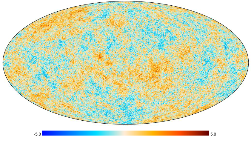
Refer to caption
Refer to caption
Refer to caption
Figure 1: Signal plus noise maps: Upper panel is an equal area stereographic projection (the so called Mollweide projection) of the signal plus noise simulation before needlet filtering The color map is given in standardized RMS units. Bottom left panel is a gnomonic projection of the unfiltered map around a point source with 5 degree diameter; bottom right panel is a similar gnomonic projection around the same point source but from a Mexican needlet filtered map. The Mexican needlet parameters used are j=38𝑗38j=38, B=1.2𝐡1.2B=1.2 and p=1𝑝1p=1. The red marks have been added only to visualize the location of the point sources but are not part of the simulation.

6.3 Distribution of peak heights
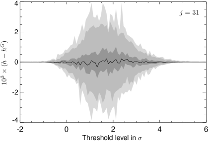
Refer to caption
Refer to caption
Refer to caption
Refer to caption
Figure 2: Peaks PDF: probability density of height of local maxima. In the upper panels, the red curves represent the analytical values, while the black curves and the gray contours are the mean and the 68,95,99 % percentiles from the simulations from 100 Monte Carlo simulations with no point sources. The lower panels show the difference between the analytical (hGsuperscriptβ„ŽπΊh^{G}) and numerical (hβ„Žh) result. The mexican needlet parameters used are p=1𝑝1p=1, B=1.2𝐡1.2B=1.2 and j=31,34𝑗3134j=31,34, which corresponds to central multipoles of β„“=[284,492]β„“284492\ell=[284,492].

The theoretical distribution of local maxima (peaks) on a Mexican needlet filtered Gaussian map is given by Eqn.  (4.10). In Fig. (2) we present the comparison of the theoretical density, hj​(x)subscriptβ„Žπ‘—π‘₯h_{j}(x), with what we obtained empirically using 100 Gaussian map simulations with no point sources. The upper panels from left to right respectively present the normalized Gaussian peak PDFs for needlet frequency j=31,34𝑗3134j=31,34, with Mexican needlet parameters B=1.2𝐡1.2B=1.2 and p=1𝑝1p=1. We chose these values as a natural compromise which on one hand illustrates higher multipoles behaviour, on the other hand still allows for extremely good numerical accuracy (better than 1% precision for finding peaks).

In the lower panel of Fig. (2) we show the relative percentage difference between the analytical and simulation results. It is easy to see from these figures that the theory fits the numerical results remarkably well. Moreover, the dispersion around the expected value of the PDF decreases as j𝑗j increases, consistently with the ergodicity result of Theorem 5.5.

6.4 Application of the STEM algorithm

The first step in the STEM algorithm, after needlet filtering, is to normalize the map using its standard deviation, as defined in Eqn.  (3.8), to obtain Eqn.  (3.9).

To find local peaks on a map we compute the first and second derivatives using HEALpix ’s routine alm2map_der. The pixels where the first derivative is close to zero (within a precision of 10βˆ’6superscript10610^{-6}) are classified as the local extrema. We then partition these extrema into maxima, minima and saddle using the eigenvalue decomposition of the Hessian matrix - of course, maxima are those with all the eigenvalues negative.

It is instructive to look at how the brightness of point sources increase as we filter the signal plus noise map with Mexican needlets. In Fig. (3), we plot the PDF of point source amplitudes before adding noise (grey curve), after adding noise but before needlet filtering (thick black curve), and after filtering with increasing j𝑗j. For the high frequency Mexican needlet we considered, j=38𝑗38j=38, filtering increases the brightness by a factor greater than 4. The negative values in the histogram are due to the added Gaussian noise; we do not expect to detect such weak sources based on their amplitude information only.
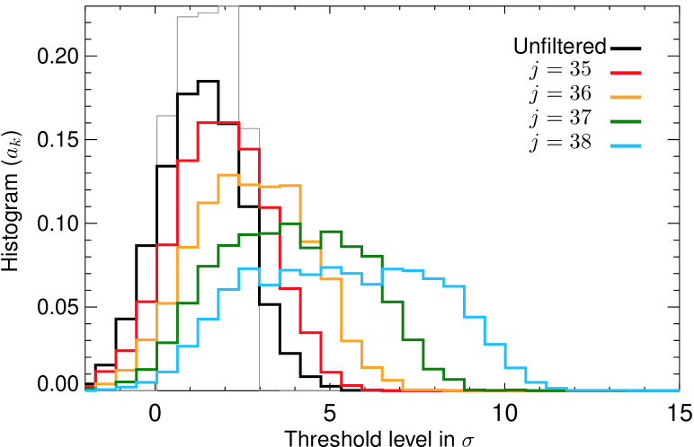
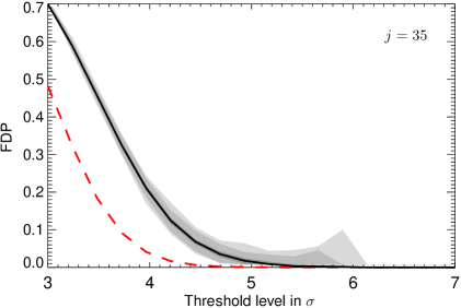
Refer to caption
Figure 3: Needlet filtering increases signal-to-noise ratio: Histogram of signal amplitudes at the location of the point sources, before adding noise (grey curve), after adding noise but before filtering (thick black curve), and after filtering with the Mexican needlet at different j𝑗j. The Mexican needlet parameters used are B=1.2𝐡1.2B=1.2 and p=1𝑝1p=1.
Refer to caption
Refer to caption
Refer to caption
Refer to caption
Figure 4: False Discovery Proportion: FDP as a function of threshold (in units of standard deviation) for different needlet scales. The dashed red curves are for the analytical upper bounds while the black curves are for the mean of the empirical FDPs from 100 Monte Carlo simulations. The gray shades are for percentiles 68,95689568,95 and 99%percent9999\%. The Mexican needlet parameters used are B=1.2𝐡1.2B=1.2 and p=1𝑝1p=1.

6.5 False Discovery Proportion (FDP)

In Eqn.  (5.5) of Section 5 we provided the analytical result on the upper bound of the FDP as a function of the power spectrum of the noise, the total number and the spatial profile of the sources. Here we compare this result with what is obtained from numerical simulations.

The empirical FDP is computed using the following steps: locate maxima on needlet filtered signal-plus-noise Monte Carlo simulations using our peak detection code; classify peaks as True discovery if the location of a maxima corresponds to a known (input) point source within ρ𝜌\rho pixel radius or False discovery if there are no input sources within ρ𝜌\rho pixels radius of the peak (ρ𝜌\rho corresponding to the tolerance parameter); count the number of True and False discoveries as a function of ρ𝜌\rho and the RMS of the noise.

Refer to caption
Refer to caption
Refer to caption
Refer to caption
Figure 5: False Discovery Rate: FDR as a function of error rate α𝛼\alpha for different needlet scales. The red curve is a plot of Ξ±βˆ—F​D​P​(u=3)𝛼𝐹𝐷𝑃𝑒3\alpha*FDP(u=3), while the black curve is the mean from 100 Monte Carlo simulations. The gray shades are for percentiles 68,95689568,95 and 99%percent9999\%. The number of point sources is 5000. The Mexican needlet parameters used are B=1.2𝐡1.2B=1.2 and p=1𝑝1p=1.

The empirical FDP as a function of u𝑒u, which is in units of the RMS of the noise, and the source detection tolerance parameter ρ𝜌\rho is computed, according to (4.5), as

FDP^ρj​(u)=# of False discoveries above ​utotal # of peaks above ​usubscript^FDPsubscriptπœŒπ‘—π‘’# of False discoveries above 𝑒total # of peaks above 𝑒\widehat{\mathrm{FDP}}_{\rho_{j}}(u)=\frac{\text{\# of False discoveries above\,}u}{\text{total \# of peaks above\,}u} (6.2)

In Fig. (4) we illustrate the comparison of the FDP for thresholds in the filtered map above 3​σ3𝜎3\sigma and ρ=3𝜌3\rho=3 for different values of j𝑗j. We found that setting 2≀ρ≀82𝜌82\leq\rho\leq 8 does not alter significantly our results (note that the smallest practical radius is ρ=2𝜌2\rho=2). The red curve in these plots corresponds to the first term on the right hand side of Eqn.  (5.5), while the black curve is from the mean of the simulations. The contours from dark to light gray corresponds to the 68,95689568,95 and 99%percent9999\% confidence intervals. We note that, as expected, the analytic results for the upper bound become larger than the numerical simulations as j𝑗j increases.

Refer to caption
Refer to caption
Figure 6: Theoretical vs numerical results for FDP and FDR: FDP as a function of thresholds and FDR as a function of global p-value, α𝛼\alpha, for needlet scale j=38𝑗38j=38. The dashed curves are the analytical upper bounds while the solid curves are the corresponding empirical results from 100 Monte Carlo simulations. The Mexican needlet parameters used are B=1.2𝐡1.2B=1.2 and p=1𝑝1p=1

6.6 False Discovery Rate (FDR)

We now proceed in validating the analytical formalism established in Section 5 to control the false discovery rate (FDR). This is done by comparing the analytical upper bound of the FDR, which is given by Eqn.  (5.5), with the empirical result from simulations. In Fig. (5), it is shown that for a given error rate, the empirical FDR is always below the upper limit set by the theory.

In Fig. (6) we present the mean FDP and FDR curves together with the corresponding theoretical results for different number of input sources. Again, the FDP and FDR are bounded above by the theoretical bounds.

6.7 Detection power

To quantify how many of the input point sources we discovered in our analysis, in Fig. (7) we show the number of peaks that matches the true sources i.e., the numerator of (4.7), which measures the statistical power of the algorithm. These results show that the power of the STEM algorithm is almost 100% in detecting bright sources - indeed, we have detected all input sources whose brightness was above 1​σ1𝜎1\sigma in the unfiltered simulated maps.

Overall, we believe that the results in this section provide a strong numerical support for the asymptotic findings that we described earlier in this paper.
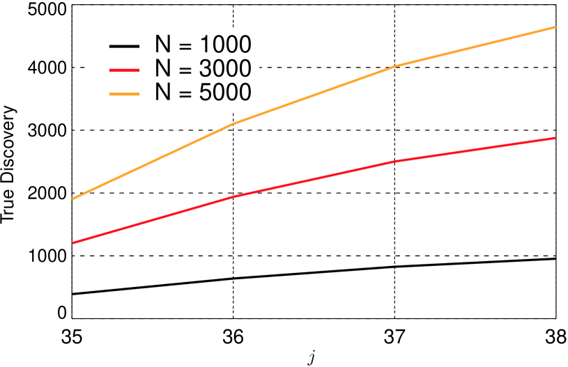
Refer to caption
Figure 7: Detection power: number of true discoveries for threshold u>3𝑒3u>3 as a function of needlet scales, j𝑗j. The three curves are the mean of 100 Monte Carlo simulations for the corresponding cases. The legend shows the number of input point sources in simulations. The Mexican needlet parameters used are B=1.2𝐡1.2B=1.2 and p=1𝑝1p=1.

Appendix A Proof of Theorem 5.5

A.1 Voronoi cells

We introduce the following notation for the spherical caps in π•Š2superscriptπ•Š2\mathbb{S}^{2}:

ℬ​(a,Ξ΅)={xβŠ†π•Š2:d​(a,x)≀Ρ}.β„¬π‘Žπœ€conditional-setπ‘₯superscriptπ•Š2π‘‘π‘Žπ‘₯πœ€\displaystyle\mathcal{B}(a,\varepsilon)=\{x\subseteq\mathbb{S}^{2}:d(a,x)\leq\varepsilon\}.

For any Ξ΅>0πœ€0\varepsilon>0, we say that ΞΡ={ΞΎ1,Ξ΅,…,ΞΎN,Ξ΅}subscriptΞžπœ€subscriptπœ‰1πœ€β€¦subscriptπœ‰π‘πœ€\Xi_{\varepsilon}=\{\xi_{1,\varepsilon},\dots,\xi_{N,\varepsilon}\} is a maximal Ξ΅πœ€\varepsilon-net, if ΞΎ1,Ξ΅,…,ΞΎN,Ξ΅subscriptπœ‰1πœ€β€¦subscriptπœ‰π‘πœ€\xi_{1,\varepsilon},\dots,\xi_{N,\varepsilon} are in π•Š2superscriptπ•Š2\mathbb{S}^{2}, βˆ€iβ‰ jfor-all𝑖𝑗\forall i\neq j we have d​(ΞΎi,Ξ΅,ΞΎj,Ξ΅)>Ρ𝑑subscriptπœ‰π‘–πœ€subscriptπœ‰π‘—πœ€πœ€d(\xi_{i,\varepsilon},\xi_{j,\varepsilon})>\varepsilon and βˆ€xβˆˆπ•Š2,d​(x,ΞΡ)≀Ρ.formulae-sequencefor-allπ‘₯superscriptπ•Š2𝑑π‘₯subscriptΞžπœ€πœ€\forall x\in\mathbb{S}^{2},\;\;d(x,\Xi_{\varepsilon})\leq\varepsilon. Heuristically, an Ξ΅πœ€\varepsilon-net is a grid of point at a distance at least Ξ΅πœ€\varepsilon from each other, and such that any extra point should be within a distance Ξ΅πœ€\varepsilon from a point in the grid, see [5, Lemma 5]. The number N𝑁N of points in a Ξ΅πœ€\varepsilon-net on the sphere can be bounded from above and from below, indeed we have the following:

4Ξ΅2≀N≀4Ξ΅2​π2.4superscriptπœ€2𝑁4superscriptπœ€2superscriptπœ‹2\frac{4}{\varepsilon^{2}}\leq N\leq\frac{4}{\varepsilon^{2}}\pi^{2}.

Given an Ξ΅πœ€\varepsilon-net it is natural to partition the sphere into disjoint sets, each of them associated with a single point in the net. This task is accomplished by the well-known Voronoi cells construction.

Definition A.1

Let ΞΡsubscriptΞžπœ€\Xi_{\varepsilon} be a maximal Ξ΅πœ€\varepsilon-net. For all ΞΎi,Ρ∈ΞΡsubscriptπœ‰π‘–πœ€subscriptΞžπœ€\xi_{i,\varepsilon}\in\Xi_{\varepsilon}, the associated family of Voronoi cells is defined by

𝒱​(ΞΎi,Ξ΅,Ξ΅)={xβˆˆπ•Š2:βˆ€jβ‰ i,d​(x,ΞΎi,Ξ΅)≀d​(x,ΞΎj,Ξ΅)}.𝒱subscriptπœ‰π‘–πœ€πœ€conditional-setπ‘₯superscriptπ•Š2formulae-sequencefor-all𝑗𝑖𝑑π‘₯subscriptπœ‰π‘–πœ€π‘‘π‘₯subscriptπœ‰π‘—πœ€\mathcal{V}(\xi_{i,\varepsilon},\varepsilon)=\{x\in\mathbb{S}^{2}:\forall j\neq i,\;d(x,\xi_{i,\varepsilon})\leq d(x,\xi_{j,\varepsilon})\}.

We recall that ℬ​(ΞΎi,Ξ΅,Ξ΅/2)βŠ†π’±β€‹(ΞΎi,Ξ΅,Ξ΅)βŠ†β„¬β€‹(ΞΎi,Ξ΅,Ξ΅)ℬsubscriptπœ‰π‘–πœ€πœ€2𝒱subscriptπœ‰π‘–πœ€πœ€β„¬subscriptπœ‰π‘–πœ€πœ€\mathcal{B}(\xi_{i,\varepsilon},\varepsilon/2)\subseteq\mathcal{V}(\xi_{i,\varepsilon},\varepsilon)\subseteq\mathcal{B}(\xi_{i,\varepsilon},\varepsilon), hence Area​(𝒱​(ΞΎi,Ξ΅,Ξ΅))β‰ˆΞ΅2Area𝒱subscriptπœ‰π‘–πœ€πœ€superscriptπœ€2\text{Area}(\mathcal{V}(\xi_{i,\varepsilon},\varepsilon))\approx\varepsilon^{2}. Let

𝒩c​(Ξ²~j;𝒱​(ΞΎi,Ξ΅,Ξ΅),I)=#​{xβˆˆπ’±β€‹(ΞΎi,Ξ΅,Ξ΅):Ξ²~j​(x)∈I,βˆ‡Ξ²~j​(x)=0}.superscript𝒩𝑐subscript~𝛽𝑗𝒱subscriptπœ‰π‘–πœ€πœ€πΌ#conditional-setπ‘₯𝒱subscriptπœ‰π‘–πœ€πœ€formulae-sequencesubscript~𝛽𝑗π‘₯πΌβˆ‡subscript~𝛽𝑗π‘₯0\mathcal{N}^{c}(\tilde{\beta}_{j};\mathcal{V}(\xi_{i,\varepsilon},\varepsilon),I)=\#\{x\in\mathcal{V}(\xi_{i,\varepsilon},\varepsilon):\tilde{\beta}_{j}(x)\in I,\nabla\tilde{\beta}_{j}(x)=0\}.

Note that, almost surely, the sum of the critical points over the Voronoi cells equals the total number of critical points:

𝒩Ic​(Ξ²~j)=βˆ‘ΞΎi,Ξ΅βˆˆΞžΞ΅π’©c​(Ξ²~j;𝒱​(ΞΎi,Ξ΅,Ξ΅),I).subscriptsuperscript𝒩𝑐𝐼subscript~𝛽𝑗subscriptsubscriptπœ‰π‘–πœ€subscriptΞžπœ€superscript𝒩𝑐subscript~𝛽𝑗𝒱subscriptπœ‰π‘–πœ€πœ€πΌ\displaystyle\mathcal{N}^{c}_{I}(\tilde{\beta}_{j})=\sum_{\xi_{i,\varepsilon}\in\Xi_{\varepsilon}}\mathcal{N}^{c}(\tilde{\beta}_{j};\mathcal{V}(\xi_{i,\varepsilon},\varepsilon),I).

Our proof uses similar ideas to those exploited in [8] for the analysis of critical points of spherical random eigenfunctions. In particular, we split the variance into two terms, one related to the correlation between Voronoi cells which are further apart than an (asymptotically vanishing) threshold (the so-called β€œlong-range component”), the other related to Voronoi cells whose distance is smaller than the threshold.

More precisely, we have that

Var​(𝒩Ic​(Ξ²~j))Varsubscriptsuperscript𝒩𝑐𝐼subscript~𝛽𝑗\displaystyle\text{Var}\left(\mathcal{N}^{c}_{I}(\tilde{\beta}_{j})\right) =βˆ‘ΞΎi,Ξ΅,ΞΎk,Ρ∈ΞΡCov​(𝒩c​(Ξ²~j;𝒱​(ΞΎi,Ξ΅),I),𝒩c​(Ξ²~j;𝒱​(ΞΎk,Ξ΅),I))absentsubscriptsubscriptπœ‰π‘–πœ€subscriptπœ‰π‘˜πœ€subscriptΞžπœ€Covsuperscript𝒩𝑐subscript~𝛽𝑗𝒱subscriptπœ‰π‘–πœ€πΌsuperscript𝒩𝑐subscript~𝛽𝑗𝒱subscriptπœ‰π‘˜πœ€πΌ\displaystyle=\sum_{\xi_{i,\varepsilon},\xi_{k,\varepsilon}\in\Xi_{\varepsilon}}\text{Cov}\left(\mathcal{N}^{c}(\tilde{\beta}_{j};\mathcal{V}(\xi_{i,\varepsilon}),I),\mathcal{N}^{c}(\tilde{\beta}_{j};\mathcal{V}(\xi_{k,\varepsilon}),I)\right)
=βˆ‘d​(𝒱​(ΞΎi,Ξ΅),𝒱​(ΞΎk,Ξ΅))>C/BjCov​(𝒩c​(Ξ²~j;𝒱​(ΞΎi,Ξ΅),I),𝒩c​(Ξ²~j;𝒱​(ΞΎk,Ξ΅),I))absentsubscript𝑑𝒱subscriptπœ‰π‘–πœ€π’±subscriptπœ‰π‘˜πœ€πΆsuperscript𝐡𝑗Covsuperscript𝒩𝑐subscript~𝛽𝑗𝒱subscriptπœ‰π‘–πœ€πΌsuperscript𝒩𝑐subscript~𝛽𝑗𝒱subscriptπœ‰π‘˜πœ€πΌ\displaystyle=\sum_{d(\mathcal{V}(\xi_{i,\varepsilon}),\mathcal{V}(\xi_{k,\varepsilon}))>C/B^{j}}\text{Cov}\left(\mathcal{N}^{c}(\tilde{\beta}_{j};\mathcal{V}(\xi_{i,\varepsilon}),I),\mathcal{N}^{c}(\tilde{\beta}_{j};\mathcal{V}(\xi_{k,\varepsilon}),I)\right) (1.1)
+βˆ‘d​(𝒱​(ΞΎi,Ξ΅),𝒱​(ΞΎk,Ξ΅))≀C/BjCov​(𝒩c​(Ξ²~j;𝒱​(ΞΎi,Ξ΅),I),𝒩c​(Ξ²~j;𝒱​(ΞΎk,Ξ΅),I)).subscript𝑑𝒱subscriptπœ‰π‘–πœ€π’±subscriptπœ‰π‘˜πœ€πΆsuperscript𝐡𝑗Covsuperscript𝒩𝑐subscript~𝛽𝑗𝒱subscriptπœ‰π‘–πœ€πΌsuperscript𝒩𝑐subscript~𝛽𝑗𝒱subscriptπœ‰π‘˜πœ€πΌ\displaystyle\;\;+\sum_{d(\mathcal{V}(\xi_{i,\varepsilon}),\mathcal{V}(\xi_{k,\varepsilon}))\leq C/B^{j}}\text{Cov}\left(\mathcal{N}^{c}(\tilde{\beta}_{j};\mathcal{V}(\xi_{i,\varepsilon}),I),\mathcal{N}^{c}(\tilde{\beta}_{j};\mathcal{V}(\xi_{k,\varepsilon}),I)\right). (1.2)

In Section A.2 we prove that the asymptotic behaviour of the long-range component (1.1) is

βˆ‘d​(𝒱​(ΞΎi,Ξ΅),𝒱​(ΞΎk,Ξ΅))>C/BjCov​(𝒩c​(Ξ²~j;𝒱​(ΞΎi,Ξ΅),I),𝒩c​(Ξ²~j;𝒱​(ΞΎk,Ξ΅),I))≀c1​(I)​j2​B2​j+o​(j2​B2​j)subscript𝑑𝒱subscriptπœ‰π‘–πœ€π’±subscriptπœ‰π‘˜πœ€πΆsuperscript𝐡𝑗Covsuperscript𝒩𝑐subscript~𝛽𝑗𝒱subscriptπœ‰π‘–πœ€πΌsuperscript𝒩𝑐subscript~𝛽𝑗𝒱subscriptπœ‰π‘˜πœ€πΌsubscript𝑐1𝐼superscript𝑗2superscript𝐡2π‘—π‘œsuperscript𝑗2superscript𝐡2𝑗\sum_{d(\mathcal{V}(\xi_{i,\varepsilon}),\mathcal{V}(\xi_{k,\varepsilon}))>C/B^{j}}\text{Cov}\left(\mathcal{N}^{c}(\tilde{\beta}_{j};\mathcal{V}(\xi_{i,\varepsilon}),I),\mathcal{N}^{c}(\tilde{\beta}_{j};\mathcal{V}(\xi_{k,\varepsilon}),I)\right)\leq c_{1}(I)j^{2}B^{2j}+o(j^{2}B^{2j}) (1.3)

while in Section A.3 we prove that for (1.2) we have

βˆ‘d​(𝒱​(ΞΎi,Ξ΅),𝒱​(ΞΎk,Ξ΅))≀C/BjCov​(𝒩c​(Ξ²~j;𝒱​(ΞΎi,Ξ΅),I),𝒩c​(Ξ²~j;𝒱​(ΞΎk,Ξ΅),I))≀c2​(I)​B2​j+o​(B2​j),subscript𝑑𝒱subscriptπœ‰π‘–πœ€π’±subscriptπœ‰π‘˜πœ€πΆsuperscript𝐡𝑗Covsuperscript𝒩𝑐subscript~𝛽𝑗𝒱subscriptπœ‰π‘–πœ€πΌsuperscript𝒩𝑐subscript~𝛽𝑗𝒱subscriptπœ‰π‘˜πœ€πΌsubscript𝑐2𝐼superscript𝐡2π‘—π‘œsuperscript𝐡2𝑗\sum_{d(\mathcal{V}(\xi_{i,\varepsilon}),\mathcal{V}(\xi_{k,\varepsilon}))\leq C/B^{j}}\text{Cov}\left(\mathcal{N}^{c}(\tilde{\beta}_{j};\mathcal{V}(\xi_{i,\varepsilon}),I),\mathcal{N}^{c}(\tilde{\beta}_{j};\mathcal{V}(\xi_{k,\varepsilon}),I)\right)\leq c_{2}(I)B^{2j}+o(B^{2j}), (1.4)

where c1​(I),c2​(I)subscript𝑐1𝐼subscript𝑐2𝐼c_{1}(I),c_{2}(I) are uniformly bounded for every IβŠ‚β„πΌβ„I\subset\mathbb{R}.

As in [8], let us introduce also the two-point correlation function K2,jsubscript𝐾2𝑗K_{2,j}, which is given by

K2,j​(x,y;t1,t2)=subscript𝐾2𝑗π‘₯𝑦subscript𝑑1subscript𝑑2absent\displaystyle K_{2,j}(x,y;t_{1},t_{2})= 𝔼[|βˆ‡2Ξ²~j(x)|β‹…|βˆ‡2Ξ²~j(y)||βˆ‡Ξ²~j(x)=βˆ‡Ξ²~j(y)=0,Ξ²~j(x)=t1,Ξ²~j(y)=t2]\displaystyle\mathbb{E}\left[\left|\nabla^{2}\tilde{\beta}_{j}(x)\right|\cdot\left|\nabla^{2}\tilde{\beta}_{j}(y)\right|\Big{|}\nabla\tilde{\beta}_{j}(x)=\nabla\tilde{\beta}_{j}(y)=0,\tilde{\beta}_{j}(x)=t_{1},\tilde{\beta}_{j}(y)=t_{2}\right]
Γ—Ο†x,y​(t1,t2,0,0,0,0)absentsubscriptπœ‘π‘₯𝑦subscript𝑑1subscript𝑑20000\displaystyle\times\varphi_{x,y}(t_{1},t_{2},0,0,0,0) (1.5)

where t1,t2βˆˆβ„subscript𝑑1subscript𝑑2ℝt_{1},t_{2}\in\mathbb{R} and Ο†x,y​(t1,t2,0,0,0,0)subscriptπœ‘π‘₯𝑦subscript𝑑1subscript𝑑20000\varphi_{x,y}(t_{1},t_{2},0,0,0,0) denotes the density of the 6-dimensional vector

(Ξ²~j​(x),Ξ²~j​(y),βˆ‡Ξ²~j​(x),βˆ‡Ξ²~j​(y))subscript~𝛽𝑗π‘₯subscript~π›½π‘—π‘¦βˆ‡subscript~𝛽𝑗π‘₯βˆ‡subscript~𝛽𝑗𝑦\left(\tilde{\beta}_{j}(x),\tilde{\beta}_{j}(y),\nabla\tilde{\beta}_{j}(x),\nabla\tilde{\beta}_{j}(y)\right)

in Ξ²~j​(x)=t1,Ξ²~j​(y)=t2,βˆ‡Ξ²~j​(x)=βˆ‡Ξ²~j​(y)=𝟎formulae-sequencesubscript~𝛽𝑗π‘₯subscript𝑑1formulae-sequencesubscript~𝛽𝑗𝑦subscript𝑑2βˆ‡subscript~𝛽𝑗π‘₯βˆ‡subscript~𝛽𝑗𝑦0\tilde{\beta}_{j}(x)=t_{1},\tilde{\beta}_{j}(y)=t_{2},\nabla\tilde{\beta}_{j}(x)=\nabla\tilde{\beta}_{j}(y)=\mathbf{0}. Note that, by isotropy, the function K2,jsubscript𝐾2𝑗K_{2,j} depends on the points xπ‘₯x, y𝑦y only through their geodesic distance Ο•=d​(x,y)italic-ϕ𝑑π‘₯𝑦\phi=d(x,y); with some abuse of notation, we shall write

K2,j​(Ο•;t1,t2)=K2,j​(x,y;t1,t2).subscript𝐾2𝑗italic-Ο•subscript𝑑1subscript𝑑2subscript𝐾2𝑗π‘₯𝑦subscript𝑑1subscript𝑑2K_{2,j}(\phi;t_{1},t_{2})=K_{2,j}(x,y;t_{1},t_{2}).

We are now in the position to investigate the asymptotic behaviour of the long- and short-range components, respectively.

A.2 Proof of the long-range asymptotic bound (1.3)

By the Kac-Rice expectation metatheorem (see i.e., [1], Chapter 11), we have

βˆ‘d​(𝒱​(ΞΎi,Ξ΅),𝒱​(ΞΎk,Ξ΅))>C/BjCov​(𝒩c​(Ξ²~j;𝒱​(ΞΎi,Ξ΅),I),𝒩c​(Ξ²~j;𝒱​(ΞΎk,Ξ΅),I))subscript𝑑𝒱subscriptπœ‰π‘–πœ€π’±subscriptπœ‰π‘˜πœ€πΆsuperscript𝐡𝑗Covsuperscript𝒩𝑐subscript~𝛽𝑗𝒱subscriptπœ‰π‘–πœ€πΌsuperscript𝒩𝑐subscript~𝛽𝑗𝒱subscriptπœ‰π‘˜πœ€πΌ\displaystyle\sum_{d(\mathcal{V}(\xi_{i,\varepsilon}),\mathcal{V}(\xi_{k,\varepsilon}))>C/B^{j}}\text{Cov}\left(\mathcal{N}^{c}(\tilde{\beta}_{j};\mathcal{V}(\xi_{i,\varepsilon}),I),\mathcal{N}^{c}(\tilde{\beta}_{j};\mathcal{V}(\xi_{k,\varepsilon}),I)\right)
=βˆ«π’²βˆ«IΓ—IK2,j​(x,y;t1,t2)​𝑑t1​𝑑t2​𝑑x​𝑑yβˆ’π”Όβ€‹[𝒩c​(Ξ²~j;𝒱​(ΞΎi,Ξ΅),I)]​𝔼​[𝒩c​(Ξ²~j;𝒱​(ΞΎk,Ξ΅),I)]absentsubscript𝒲subscript𝐼𝐼subscript𝐾2𝑗π‘₯𝑦subscript𝑑1subscript𝑑2differential-dsubscript𝑑1differential-dsubscript𝑑2differential-dπ‘₯differential-d𝑦𝔼delimited-[]superscript𝒩𝑐subscript~𝛽𝑗𝒱subscriptπœ‰π‘–πœ€πΌπ”Όdelimited-[]superscript𝒩𝑐subscript~𝛽𝑗𝒱subscriptπœ‰π‘˜πœ€πΌ\displaystyle\hskip 42.67912pt=\int_{\mathcal{W}}\int_{I\times I}K_{2,j}(x,y;t_{1},t_{2})dt_{1}dt_{2}dxdy-\mathbb{E}[\mathcal{N}^{c}(\tilde{\beta}_{j};\mathcal{V}(\xi_{i,\varepsilon}),I)]\mathbb{E}[\mathcal{N}^{c}(\tilde{\beta}_{j};\mathcal{V}(\xi_{k,\varepsilon}),I)]

where

𝒲=⋃d​(𝒱​(ΞΎi,Ξ΅),𝒱​(ΞΎk,Ξ΅))>C/Bj𝒱​(ΞΎi,Ξ΅)×𝒱​(ΞΎk,Ξ΅),𝒲subscript𝑑𝒱subscriptπœ‰π‘–πœ€π’±subscriptπœ‰π‘˜πœ€πΆsuperscript𝐡𝑗𝒱subscriptπœ‰π‘–πœ€π’±subscriptπœ‰π‘˜πœ€\mathcal{W}=\bigcup_{d(\mathcal{V}(\xi_{i,\varepsilon}),\mathcal{V}(\xi_{k,\varepsilon}))>C/B^{j}}\mathcal{V}(\xi_{i,\varepsilon})\times\mathcal{V}(\xi_{k,\varepsilon}),

is the union of Voronoi cells which are further away than C/Bj𝐢superscript𝐡𝑗C/B^{j}. Our next result is a convenient expression for the expectation; here and in the sequel, we use the simplified notation

ℬ2​n=ℬ2​n,j=ℬ2​n,p,j,subscriptℬ2𝑛subscriptℬ2𝑛𝑗subscriptℬ2𝑛𝑝𝑗{\cal B}_{2n}={\cal B}_{2n,j}={\cal B}_{2n,p,j},

where ℬ2​n,p,jsubscriptℬ2𝑛𝑝𝑗{\cal B}_{2n,p,j} was introduced in (3.2).

Lemma A.2
𝔼​[𝒩Ic​(Ξ²~j​(x))]=12​ℬ4,jℬ2,jβ€‹βˆ«Ip​(t)​𝑑t,𝔼delimited-[]superscriptsubscript𝒩𝐼𝑐subscript~𝛽𝑗π‘₯12subscriptℬ4𝑗subscriptℬ2𝑗subscript𝐼𝑝𝑑differential-d𝑑\displaystyle\mathbb{E}[\mathcal{N}_{I}^{c}(\tilde{\beta}_{j}(x))]=\frac{1}{2}\frac{\mathcal{B}_{4,j}}{\mathcal{B}_{2,j}}\int_{I}p(t)dt,

where the function p𝑝p is defined in (1.6).

ProofΒ Β Let 𝒩Ic​(Ξ²~j)superscriptsubscript𝒩𝐼𝑐subscript~𝛽𝑗\mathcal{N}_{I}^{c}(\tilde{\beta}_{j}) be the number of critical points with value in I𝐼I

𝒩Ic​(Ξ²~j)superscriptsubscript𝒩𝐼𝑐subscript~𝛽𝑗\displaystyle\mathcal{N}_{I}^{c}(\tilde{\beta}_{j}) =#​{x∈S2:Ξ²~j​(x)∈I,βˆ‡Ξ²~j​(x)=0}.absent#conditional-setπ‘₯superscript𝑆2formulae-sequencesubscript~𝛽𝑗π‘₯πΌβˆ‡subscript~𝛽𝑗π‘₯0\displaystyle=\#\{x\in{S^{2}}:\tilde{\beta}_{j}(x)\in I,\nabla\tilde{\beta}_{j}(x)=0\}.

From isotropy and Kac-Rice metatheorem we immediately get that

𝔼​[𝒩Ic​(Ξ²~j​(x))]𝔼delimited-[]superscriptsubscript𝒩𝐼𝑐subscript~𝛽𝑗π‘₯\displaystyle\mathbb{E}[\mathcal{N}_{I}^{c}(\tilde{\beta}_{j}(x))] =4β€‹Ο€β€‹βˆ«β„4|ΞΆ1​΢3βˆ’ΞΆ22|β€‹πŸ™{t∈I}​Dj​(t,0,0,ΞΆ1,ΞΆ2,ΞΆ3)​𝑑t​𝑑΢1​𝑑΢2​𝑑΢3absent4πœ‹subscriptsuperscriptℝ4subscript𝜁1subscript𝜁3superscriptsubscript𝜁22subscript1𝑑𝐼subscript𝐷𝑗𝑑00subscript𝜁1subscript𝜁2subscript𝜁3differential-d𝑑differential-dsubscript𝜁1differential-dsubscript𝜁2differential-dsubscript𝜁3\displaystyle=4\pi\int_{\mathbb{R}^{4}}|\zeta_{1}\zeta_{3}-\zeta_{2}^{2}|\mathbbm{1}_{\{t\in I\}}D_{j}(t,0,0,\zeta_{1},\zeta_{2},\zeta_{3})dt\;d\zeta_{1}\;d\zeta_{2}\;d\zeta_{3}

where Dj​(t,0,0,ΞΆ1,ΞΆ2,ΞΆ3)subscript𝐷𝑗𝑑00subscript𝜁1subscript𝜁2subscript𝜁3D_{j}(t,0,0,\zeta_{1},\zeta_{2},\zeta_{3}) denotes the joint density of (Ξ²~j​(x),βˆ‡Ξ²~j​(x),βˆ‡2Ξ²~j​(x))subscript~𝛽𝑗π‘₯βˆ‡subscript~𝛽𝑗π‘₯superscriptβˆ‡2subscript~𝛽𝑗π‘₯(\tilde{\beta}_{j}(x),\nabla\tilde{\beta}_{j}(x),\nabla^{2}\tilde{\beta}_{j}(x)) in Ξ²~j​(x)=tsubscript~𝛽𝑗π‘₯𝑑\tilde{\beta}_{j}(x)=t, βˆ‡Ξ²~j​(x)=πŸŽβˆ‡subscript~𝛽𝑗π‘₯0\nabla\tilde{\beta}_{j}(x)=\mathbf{0}, βˆ‡2Ξ²~j​(x)=(ΞΆ1,ΞΆ2,ΞΆ3)=ΞΆsuperscriptβˆ‡2subscript~𝛽𝑗π‘₯subscript𝜁1subscript𝜁2subscript𝜁3𝜁\nabla^{2}\tilde{\beta}_{j}(x)=(\zeta_{1},\zeta_{2},\zeta_{3})={\zeta}. Since, at each fixed xπ‘₯x, first and second derivatives are uncorrelated we have

Dj​(t,0,0,ΞΆ1,ΞΆ2,ΞΆ3)=Dj,1​(0,0)​Dj,2​(t)​Dj,3​(ΞΆ1,ΞΆ2,ΞΆ3|Ξ²~j​(x)=t),subscript𝐷𝑗𝑑00subscript𝜁1subscript𝜁2subscript𝜁3subscript𝐷𝑗100subscript𝐷𝑗2𝑑subscript𝐷𝑗3subscript𝜁1subscript𝜁2conditionalsubscript𝜁3subscript~𝛽𝑗π‘₯𝑑D_{j}(t,0,0,\zeta_{1},\zeta_{2},\zeta_{3})=D_{j,1}(0,0)D_{j,2}(t)D_{j,3}(\zeta_{1},\zeta_{2},\zeta_{3}|\tilde{\beta}_{j}(x)=t),

where Dj,1subscript𝐷𝑗1D_{j,1}, Dj,2subscript𝐷𝑗2D_{j,2} and Dj,3subscript𝐷𝑗3D_{j,3} are the marginal densities of βˆ‡Ξ²~j​(x)βˆ‡subscript~𝛽𝑗π‘₯\nabla\tilde{\beta}_{j}(x), Ξ²~j​(x)subscript~𝛽𝑗π‘₯\tilde{\beta}_{j}(x) and (βˆ‡2Ξ²~j​(x)|Ξ²~j​(x)=t)conditionalsuperscriptβˆ‡2subscript~𝛽𝑗π‘₯subscript~𝛽𝑗π‘₯𝑑(\nabla^{2}\tilde{\beta}_{j}(x)|\tilde{\beta}_{j}(x)=t) respectively. In view of the results in Section B, we immediately have that

Dj,1​(0,0)=12​π​114​ℬ2,j2=12​π​1ℬ2,j2,Dj,2​(t)=12​π​eβˆ’t22,formulae-sequencesubscript𝐷𝑗10012πœ‹114subscriptsuperscriptℬ22𝑗12πœ‹1subscriptℬ2𝑗2subscript𝐷𝑗2𝑑12πœ‹superscript𝑒superscript𝑑22D_{j,1}(0,0)=\frac{1}{2\pi}\frac{1}{\sqrt{\frac{1}{4}\mathcal{B}^{2}_{2,j}}}=\frac{1}{2\pi}\frac{1}{\frac{\mathcal{B}_{2,j}}{2}},\hskip 28.45274ptD_{j,2}(t)=\frac{1}{\sqrt{2\pi}}e^{-\frac{t^{2}}{2}},

and

Dj,3​(ΞΆ1,ΞΆ2,ΞΆ3|Ξ²~j​(x)=t)=1(2​π)3/2​det​(Ο‰j)​exp⁑{βˆ’12​(ΞΆβˆ’ΞΌj​(t))​ωjβˆ’1​(ΞΆβˆ’ΞΌj​(t))t}subscript𝐷𝑗3subscript𝜁1subscript𝜁2conditionalsubscript𝜁3subscript~𝛽𝑗π‘₯𝑑1superscript2πœ‹32detsubscriptπœ”π‘—12𝜁subscriptπœ‡π‘—π‘‘subscriptsuperscriptπœ”1𝑗superscript𝜁subscriptπœ‡π‘—π‘‘π‘‘\displaystyle D_{j,3}(\zeta_{1},\zeta_{2},\zeta_{3}|\tilde{\beta}_{j}(x)=t)=\frac{1}{(2\pi)^{3/2}\sqrt{\text{det}(\omega_{j})}}\exp\{-\frac{1}{2}({\zeta}-\mu_{j}(t))\omega^{-1}_{j}({\zeta}-\mu_{j}(t))^{t}\}

where

ΞΌj​(t)=(βˆ’t2​ℬ2,j0βˆ’t2​ℬ2,j),Ο‰j=(38​ℬ4,jβˆ’14​ℬ2,jβˆ’14​ℬ2,j2018​ℬ4,j+14​ℬ2,jβˆ’14​ℬ2,j2018​ℬ4,jβˆ’14​ℬ2,j018​ℬ4,j+14​ℬ2,jβˆ’14​ℬ2,j2038​ℬ4,jβˆ’14​ℬ2,jβˆ’14​ℬ2,j2).formulae-sequencesubscriptπœ‡π‘—π‘‘π‘‘2subscriptℬ2𝑗0𝑑2subscriptℬ2𝑗subscriptπœ”π‘—38subscriptℬ4𝑗14subscriptℬ2𝑗14subscriptsuperscriptℬ22𝑗018subscriptℬ4𝑗14subscriptℬ2𝑗14subscriptsuperscriptℬ22𝑗018subscriptℬ4𝑗14subscriptℬ2𝑗018subscriptℬ4𝑗14subscriptℬ2𝑗14subscriptsuperscriptℬ22𝑗038subscriptℬ4𝑗14subscriptℬ2𝑗14subscriptsuperscriptℬ22𝑗\displaystyle\mu_{j}(t)=\left(\begin{array}[]{c}-\frac{t}{2}\mathcal{B}_{2,j}\\ 0\\ -\frac{t}{2}\mathcal{B}_{2,j}\end{array}\right),\hskip 14.22636pt\omega_{j}=\left(\begin{array}[]{ccc}\frac{3}{8}\mathcal{B}_{4,j}-\frac{1}{4}\mathcal{B}_{2,j}-\frac{1}{4}\mathcal{B}^{2}_{2,j}&0&\frac{1}{8}\mathcal{B}_{4,j}+\frac{1}{4}\mathcal{B}_{2,j}-\frac{1}{4}\mathcal{B}^{2}_{2,j}\\ 0&\frac{1}{8}\mathcal{B}_{4,j}-\frac{1}{4}\mathcal{B}_{2,j}&0\\ \frac{1}{8}\mathcal{B}_{4,j}+\frac{1}{4}\mathcal{B}_{2,j}-\frac{1}{4}\mathcal{B}^{2}_{2,j}&0&\frac{3}{8}\mathcal{B}_{4,j}-\frac{1}{4}\mathcal{B}_{2,j}-\frac{1}{4}\mathcal{B}^{2}_{2,j}\end{array}\right).

With the scaling 8ℬ4,j​(βˆ‡2Ξ²~j|Ξ²~j)∼N​(ΞΌ~j​(t),Ο‰~j)similar-to8subscriptℬ4𝑗conditionalsuperscriptβˆ‡2subscript~𝛽𝑗subscript~𝛽𝑗𝑁subscript~πœ‡π‘—π‘‘subscript~πœ”π‘—\frac{\sqrt{8}}{\sqrt{\mathcal{B}_{4,j}}}(\nabla^{2}\tilde{\beta}_{j}|\tilde{\beta}_{j})\sim N(\tilde{\mu}_{j}(t),\tilde{\omega}_{j}), where ΞΌ~j​(t)=8ℬ4,j​μj​(t)subscript~πœ‡π‘—π‘‘8subscriptℬ4𝑗subscriptπœ‡π‘—π‘‘\tilde{\mu}_{j}(t)=\frac{\sqrt{8}}{\sqrt{\mathcal{B}_{4,j}}}\mu_{j}(t) and Ο‰~j=8ℬ4,j​ωjsubscript~πœ”π‘—8subscriptℬ4𝑗subscriptπœ”π‘—\tilde{\omega}_{j}=\frac{8}{{\mathcal{B}_{4,j}}}\omega_{j}, we obtain

Dj​(t,0,0,ΞΆ1,ΞΆ2,ΞΆ3)​d​t​d​΢1​d​΢2​d​΢3subscript𝐷𝑗𝑑00subscript𝜁1subscript𝜁2subscript𝜁3𝑑𝑑𝑑subscript𝜁1𝑑subscript𝜁2𝑑subscript𝜁3\displaystyle D_{j}(t,0,0,\zeta_{1},\zeta_{2},\zeta_{3})dt\;d\zeta_{1}\;d\zeta_{2}\;d\zeta_{3}
=12​π​1ℬ22​12​π​eβˆ’t22​1(2​π)3/2​det​(Ο‰~j)​exp⁑{βˆ’12​(ΞΆ~βˆ’ΞΌ~j​(t))​ω~jβˆ’1​(ΞΆ~βˆ’ΞΌ~j​(t))t}​d​t​d​΢~1​d​΢~2​d​΢~3absent12πœ‹1subscriptℬ2212πœ‹superscript𝑒superscript𝑑221superscript2πœ‹32detsubscript~πœ”π‘—12~𝜁subscript~πœ‡π‘—π‘‘superscriptsubscript~πœ”π‘—1superscript~𝜁subscript~πœ‡π‘—π‘‘π‘‘π‘‘π‘‘π‘‘subscript~𝜁1𝑑subscript~𝜁2𝑑subscript~𝜁3\displaystyle=\frac{1}{2\pi}\frac{1}{\frac{\mathcal{B}_{2}}{2}}\frac{1}{\sqrt{2\pi}}e^{-\frac{t^{2}}{2}}\frac{1}{(2\pi)^{3/2}\sqrt{\text{det}(\tilde{\omega}_{j})}}\exp\{-\frac{1}{2}(\tilde{\zeta}-\tilde{\mu}_{j}(t))\tilde{\omega}_{j}^{-1}(\tilde{\zeta}-\tilde{\mu}_{j}(t))^{t}\}dtd\tilde{\zeta}_{1}d\tilde{\zeta}_{2}d\tilde{\zeta}_{3}

and then

βˆ«β„4|ΞΆ1​΢3βˆ’ΞΆ22|β€‹πŸ™{t∈I}​Dj​(t,0,0,ΞΆ1,ΞΆ2,ΞΆ3)​𝑑t​𝑑΢1​𝑑΢2​𝑑΢3=ℬ4,j8​ℬj;22​12β€‹Ο€β€‹βˆ«Ip​(t)​𝑑t,subscriptsuperscriptℝ4subscript𝜁1subscript𝜁3superscriptsubscript𝜁22subscript1𝑑𝐼subscript𝐷𝑗𝑑00subscript𝜁1subscript𝜁2subscript𝜁3differential-d𝑑differential-dsubscript𝜁1differential-dsubscript𝜁2differential-dsubscript𝜁3subscriptℬ4𝑗8subscriptℬ𝑗2212πœ‹subscript𝐼𝑝𝑑differential-d𝑑\displaystyle\int_{\mathbb{R}^{4}}|\zeta_{1}\zeta_{3}-\zeta_{2}^{2}|\mathbbm{1}_{\{t\in I\}}D_{j}(t,0,0,\zeta_{1},\zeta_{2},\zeta_{3})dtd\zeta_{1}d\zeta_{2}d\zeta_{3}=\frac{\mathcal{B}_{4,j}}{8\frac{\mathcal{B}_{j;2}}{2}}\frac{1}{2\pi}\int_{I}p(t)dt,

with

p​(t)=12​π​1(2​π)3/2​1det​(Ο‰~j)β€‹βˆ«β„3|ΞΆ~1​΢~3βˆ’ΞΆ~22|​eβˆ’t22​exp⁑{βˆ’12​(ΞΆ~βˆ’ΞΌ~j​(t))​ω~jβˆ’1​(ΞΆ~βˆ’ΞΌ~j​(t))t}​𝑑΢~1​𝑑΢~2​𝑑΢~3.𝑝𝑑12πœ‹1superscript2πœ‹321detsubscript~πœ”π‘—subscriptsuperscriptℝ3subscript~𝜁1subscript~𝜁3superscriptsubscript~𝜁22superscript𝑒superscript𝑑2212~𝜁subscript~πœ‡π‘—π‘‘superscriptsubscript~πœ”π‘—1superscript~𝜁subscript~πœ‡π‘—π‘‘π‘‘differential-dsubscript~𝜁1differential-dsubscript~𝜁2differential-dsubscript~𝜁3\displaystyle p(t)=\frac{1}{\sqrt{2\pi}}\frac{1}{(2\pi)^{3/2}}\frac{1}{\sqrt{\text{det}(\tilde{\omega}_{j})}}\int_{\mathbb{R}^{3}}|\tilde{\zeta}_{1}\tilde{\zeta}_{3}-\tilde{\zeta}_{2}^{2}|e^{-\frac{t^{2}}{2}}\exp\{-\frac{1}{2}(\tilde{\zeta}-\tilde{\mu}_{j}(t))\tilde{\omega}_{j}^{-1}(\tilde{\zeta}-\tilde{\mu}_{j}(t))^{t}\}d\tilde{\zeta}_{1}d\tilde{\zeta}_{2}d\tilde{\zeta}_{3}. (1.6)

β–‘β–‘\square

In order to bound the variance we need to prove the following:

16​π2β€‹βˆ¬IΓ—I∫C/BjΟ€2K2,j​(Ο•;t1,t2)​sin⁑ϕ​d​ϕ​d​t1​d​t2βˆ’14​ℬ4,j2ℬ2,j2β€‹βˆ¬IΓ—Ip​(t1)​p​(t2)​𝑑t1​𝑑t216superscriptπœ‹2subscriptdouble-integral𝐼𝐼superscriptsubscript𝐢superscriptπ΅π‘—πœ‹2subscript𝐾2𝑗italic-Ο•subscript𝑑1subscript𝑑2italic-ϕ𝑑italic-ϕ𝑑subscript𝑑1𝑑subscript𝑑214subscriptsuperscriptℬ24𝑗subscriptsuperscriptℬ22𝑗subscriptdouble-integral𝐼𝐼𝑝subscript𝑑1𝑝subscript𝑑2differential-dsubscript𝑑1differential-dsubscript𝑑2\displaystyle 16\pi^{2}\iint_{I\times I}\int_{C/B^{j}}^{\frac{\pi}{2}}K_{2,j}(\phi;t_{1},t_{2})\sin\phi d\phi dt_{1}dt_{2}-\frac{1}{4}\frac{\mathcal{B}^{2}_{4,j}}{\mathcal{B}^{2}_{2,j}}\iint_{I\times I}p(t_{1})p(t_{2})dt_{1}dt_{2}
≀c1​(I)​j2​B2​j+o​(j2​B2​j)absentsubscript𝑐1𝐼superscript𝑗2superscript𝐡2π‘—π‘œsuperscript𝑗2superscript𝐡2𝑗\displaystyle\;\;\leq c_{1}(I)j^{2}B^{2j}+o(j^{2}B^{2j}) (1.7)

as jβ†’βˆžβ†’π‘—j\to\infty. The idea of the proof is to give a Taylor expansion of the difference between the two integrands in (A.2), see [8] for a related argument. More precisely, we start by giving the explicit expression of K2,jsubscript𝐾2𝑗K_{2,j} in terms of a Gaussian integral; indeed we write, for Ο•β‰₯C/Bjitalic-ϕ𝐢superscript𝐡𝑗\phi\geq C/B^{j},

K2,j​(Ο•;t1,t2)subscript𝐾2𝑗italic-Ο•subscript𝑑1subscript𝑑2\displaystyle K_{2,j}(\phi;t_{1},t_{2}) =βˆ¬β„3×ℝ3|ΞΆx,1​΢x,3βˆ’ΞΆx,22|​|ΞΆy,1​΢y,3βˆ’ΞΆy,22|absentsubscriptdouble-integralsuperscriptℝ3superscriptℝ3subscript𝜁π‘₯1subscript𝜁π‘₯3superscriptsubscript𝜁π‘₯22subscriptπœπ‘¦1subscriptπœπ‘¦3superscriptsubscriptπœπ‘¦22\displaystyle=\iint_{\mathbb{R}^{3}\times\mathbb{R}^{3}}|\zeta_{x,1}\zeta_{x,3}-\zeta_{x,2}^{2}||\zeta_{y,1}\zeta_{y,3}-\zeta_{y,2}^{2}|
Γ—Dj,x,y​(t1,t2,0,0,0,0,ΞΆx,1,ΞΆx,2,ΞΆx,3,ΞΆy,1,ΞΆy,2,ΞΆy,3)​d​΢x,1​d​΢x,2​d​΢x,3​d​΢y,1​d​΢y,2​d​΢y,3absentsubscript𝐷𝑗π‘₯𝑦subscript𝑑1subscript𝑑20000subscript𝜁π‘₯1subscript𝜁π‘₯2subscript𝜁π‘₯3subscriptπœπ‘¦1subscriptπœπ‘¦2subscriptπœπ‘¦3𝑑subscript𝜁π‘₯1𝑑subscript𝜁π‘₯2𝑑subscript𝜁π‘₯3𝑑subscriptπœπ‘¦1𝑑subscriptπœπ‘¦2𝑑subscriptπœπ‘¦3\displaystyle\;\;\times D_{j,x,y}(t_{1},t_{2},0,0,0,0,\zeta_{x,1},\zeta_{x,2},\zeta_{x,3},\zeta_{y,1},\zeta_{y,2},\zeta_{y,3})d\zeta_{x,1}d\zeta_{x,2}d\zeta_{x,3}d\zeta_{y,1}d\zeta_{y,2}d\zeta_{y,3}

where Dj,x,ysubscript𝐷𝑗π‘₯𝑦D_{j,x,y} denotes the joint density of (Ξ²~j​(x),Ξ²~j​(y),βˆ‡Ξ²~j​(x),βˆ‡Ξ²~j​(y),βˆ‡2Ξ²~j​(x),βˆ‡2Ξ²~j​(y))subscript~𝛽𝑗π‘₯subscript~π›½π‘—π‘¦βˆ‡subscript~𝛽𝑗π‘₯βˆ‡subscript~𝛽𝑗𝑦superscriptβˆ‡2subscript~𝛽𝑗π‘₯superscriptβˆ‡2subscript~𝛽𝑗𝑦(\tilde{\beta}_{j}(x),\tilde{\beta}_{j}(y),\nabla\tilde{\beta}_{j}(x),\nabla\tilde{\beta}_{j}(y),\nabla^{2}\tilde{\beta}_{j}(x),\nabla^{2}\tilde{\beta}_{j}(y)). We have also

Dj,x,y​(t1,t2,𝟎,𝟎,ΞΆx,ΞΆy)subscript𝐷𝑗π‘₯𝑦subscript𝑑1subscript𝑑200subscript𝜁π‘₯subscriptπœπ‘¦\displaystyle D_{j,x,y}(t_{1},t_{2},\mathbf{0},\mathbf{0},\zeta_{x},\zeta_{y}) =Dj,x,y,1​(𝟎,𝟎)​Dj,x,y,2​(t1,t2|βˆ‡Ξ²~j​(x)=βˆ‡Ξ²~j​(y)=𝟎)absentsubscript𝐷𝑗π‘₯𝑦100subscript𝐷𝑗π‘₯𝑦2subscript𝑑1conditionalsubscript𝑑2βˆ‡subscript~𝛽𝑗π‘₯βˆ‡subscript~𝛽𝑗𝑦0\displaystyle=D_{j,x,y,1}(\mathbf{0},\mathbf{0})D_{j,x,y,2}(t_{1},t_{2}|\nabla\tilde{\beta}_{j}(x)=\nabla\tilde{\beta}_{j}(y)=\mathbf{0})
Γ—Dj,x,y,3(ΞΆx,ΞΆy|Ξ²~j(x)=t1,Ξ²~j(y)=t2,βˆ‡Ξ²~j(x)=βˆ‡Ξ²~j(y)=𝟎)\displaystyle\;\;\times D_{j,x,y,3}(\zeta_{x},\zeta_{y}|\tilde{\beta}_{j}(x)=t_{1},\tilde{\beta}_{j}(y)=t_{2},\nabla\tilde{\beta}_{j}(x)=\nabla\tilde{\beta}_{j}(y)=\mathbf{0})

where Dj,x,y,1subscript𝐷𝑗π‘₯𝑦1D_{j,x,y,1} is the density of (βˆ‡Ξ²~j​(x),βˆ‡Ξ²~j​(y))βˆ‡subscript~𝛽𝑗π‘₯βˆ‡subscript~𝛽𝑗𝑦(\nabla\tilde{\beta}_{j}(x),\nabla\tilde{\beta}_{j}(y)) and Dj,x,y,2subscript𝐷𝑗π‘₯𝑦2D_{j,x,y,2}, Dj,x,y,3subscript𝐷𝑗π‘₯𝑦3D_{j,x,y,3} are the conditional densities of (Ξ²~j​(x),Ξ²~j​(y)|βˆ‡Ξ²~j​(x)=βˆ‡Ξ²~j​(y)=𝟎)subscript~𝛽𝑗π‘₯conditionalsubscript~π›½π‘—π‘¦βˆ‡subscript~𝛽𝑗π‘₯βˆ‡subscript~𝛽𝑗𝑦0(\tilde{\beta}_{j}(x),\tilde{\beta}_{j}(y)|\nabla\tilde{\beta}_{j}(x)=\nabla\tilde{\beta}_{j}(y)=\mathbf{0}) and (βˆ‡2Ξ²~j​(x),βˆ‡2Ξ²~j​(y)|Ξ²~j​(x)=t1,Ξ²~j​(y)=t2,βˆ‡Ξ²~j​(x)=βˆ‡Ξ²~j​(y)=𝟎)formulae-sequencesuperscriptβˆ‡2subscript~𝛽𝑗π‘₯conditionalsuperscriptβˆ‡2subscript~𝛽𝑗𝑦subscript~𝛽𝑗π‘₯subscript𝑑1formulae-sequencesubscript~𝛽𝑗𝑦subscript𝑑2βˆ‡subscript~𝛽𝑗π‘₯βˆ‡subscript~𝛽𝑗𝑦0(\nabla^{2}\tilde{\beta}_{j}(x),\nabla^{2}\tilde{\beta}_{j}(y)|\tilde{\beta}_{j}(x)=t_{1},\tilde{\beta}_{j}(y)=t_{2},\nabla\tilde{\beta}_{j}(x)=\nabla\tilde{\beta}_{j}(y)=\mathbf{0}) respectively.

In order to investigate the asymptotic behaviour of these densities, we need first to write the block components of the full covariance matrix of the field and its (first and second order) derivatives. In particular, we introduce the following notation for the matrix Ξ£j​(ϕ​(x,y))=Ξ£j​(Ο•)subscriptΣ𝑗italic-Ο•π‘₯𝑦subscriptΣ𝑗italic-Ο•\Sigma_{j}(\phi(x,y))=\Sigma_{j}(\phi):

Ξ£j​(Ο•)=(Rj​(Ο•)Ej​(Ο•)Dj​(Ο•)EjT​(Ο•)Aj​(Ο•)Bj​(Ο•)DjT​(Ο•)BjT​(Ο•)Cj​(Ο•)).subscriptΣ𝑗italic-Ο•subscript𝑅𝑗italic-Ο•subscript𝐸𝑗italic-Ο•subscript𝐷𝑗italic-Ο•subscriptsuperscript𝐸𝑇𝑗italic-Ο•subscript𝐴𝑗italic-Ο•subscript𝐡𝑗italic-Ο•subscriptsuperscript𝐷𝑇𝑗italic-Ο•subscriptsuperscript𝐡𝑇𝑗italic-Ο•subscript𝐢𝑗italic-Ο•\Sigma_{j}(\phi)=\left(\begin{array}[]{ccc}R_{j}(\phi)&E_{j}(\phi)&D_{j}(\phi)\\ E^{T}_{j}(\phi)&A_{j}(\phi)&B_{j}(\phi)\\ D^{T}_{j}(\phi)&B^{T}_{j}(\phi)&C_{j}(\phi)\end{array}\right).

Here, Rj​(ϕ​(x,y))subscript𝑅𝑗italic-Ο•π‘₯𝑦R_{j}(\phi(x,y)) is the 2Γ—2222\times 2 covariance matrix of (Ξ²~j​(x),Ξ²~j​(y))subscript~𝛽𝑗π‘₯subscript~𝛽𝑗𝑦(\tilde{\beta}_{j}(x),\tilde{\beta}_{j}(y)); Ej​(Ο•)subscript𝐸𝑗italic-Ο•E_{j}(\phi) is the 2Γ—4242\times 4 covariance matrix between (Ξ²~j​(x),Ξ²~j​(y))subscript~𝛽𝑗π‘₯subscript~𝛽𝑗𝑦(\tilde{\beta}_{j}(x),\tilde{\beta}_{j}(y)) and (βˆ‡Ξ²~j​(x),βˆ‡Ξ²~j​(y))βˆ‡subscript~𝛽𝑗π‘₯βˆ‡subscript~𝛽𝑗𝑦(\nabla\tilde{\beta}_{j}(x),\nabla\tilde{\beta}_{j}(y)); Dj​(Ο•)subscript𝐷𝑗italic-Ο•D_{j}(\phi) is the 2Γ—6262\times 6 covariance matrix between (Ξ²~j​(x),Ξ²~j​(y))subscript~𝛽𝑗π‘₯subscript~𝛽𝑗𝑦(\tilde{\beta}_{j}(x),\tilde{\beta}_{j}(y)) and (βˆ‡2Ξ²~j​(x),βˆ‡2Ξ²~j​(y))superscriptβˆ‡2subscript~𝛽𝑗π‘₯superscriptβˆ‡2subscript~𝛽𝑗𝑦(\nabla^{2}\tilde{\beta}_{j}(x),\nabla^{2}\tilde{\beta}_{j}(y)); Aj​(Ο•)subscript𝐴𝑗italic-Ο•A_{j}(\phi) is the 4Γ—4444\times 4 covariance matrix of (βˆ‡Ξ²~j​(x),βˆ‡Ξ²~j​(y))βˆ‡subscript~𝛽𝑗π‘₯βˆ‡subscript~𝛽𝑗𝑦(\nabla\tilde{\beta}_{j}(x),\nabla\tilde{\beta}_{j}(y)); Bj​(Ο•)subscript𝐡𝑗italic-Ο•B_{j}(\phi) is the 4Γ—6464\times 6 covariance matrix between (βˆ‡Ξ²~j​(x),βˆ‡Ξ²~j​(y))βˆ‡subscript~𝛽𝑗π‘₯βˆ‡subscript~𝛽𝑗𝑦(\nabla\tilde{\beta}_{j}(x),\nabla\tilde{\beta}_{j}(y)) and (βˆ‡2Ξ²~j​(x),βˆ‡2Ξ²~j​(y))superscriptβˆ‡2subscript~𝛽𝑗π‘₯superscriptβˆ‡2subscript~𝛽𝑗𝑦(\nabla^{2}\tilde{\beta}_{j}(x),\nabla^{2}\tilde{\beta}_{j}(y)); and finally for Cj​(Ο•)subscript𝐢𝑗italic-Ο•C_{j}(\phi) is the 6Γ—6666\times 6 covariance matrix of the vector (βˆ‡2Ξ²~j​(x),βˆ‡2Ξ²~j​(y))superscriptβˆ‡2subscript~𝛽𝑗π‘₯superscriptβˆ‡2subscript~𝛽𝑗𝑦(\nabla^{2}\tilde{\beta}_{j}(x),\nabla^{2}\tilde{\beta}_{j}(y)) (see Appendix B).

With this notation in mind, can easily give the value of the bivariate density for levels, evaluated at the origin; we have

Dj,x,y,1​(𝟎,𝟎)=1Ο€2​ℬ22​1(1βˆ’4​α12ℬ22)​(1βˆ’4​α22ℬ22),subscript𝐷𝑗π‘₯𝑦1001superscriptπœ‹2superscriptsubscriptℬ22114superscriptsubscript𝛼12superscriptsubscriptℬ2214superscriptsubscript𝛼22superscriptsubscriptℬ22D_{j,x,y,1}(\mathbf{0},\mathbf{0})=\frac{1}{\pi^{2}\mathcal{B}_{2}^{2}}\frac{1}{\sqrt{\big{(}1-4\frac{\alpha_{1}^{2}}{\mathcal{B}_{2}^{2}}\big{)}\big{(}1-4\frac{\alpha_{2}^{2}}{\mathcal{B}_{2}^{2}}\big{)}}},

where Ξ±1=Ξ±1,j​(Ο•)subscript𝛼1subscript𝛼1𝑗italic-Ο•\alpha_{1}=\alpha_{1,j}(\phi) and Ξ±2=Ξ±2,j​(Ο•)subscript𝛼2subscript𝛼2𝑗italic-Ο•\alpha_{2}=\alpha_{2,j}(\phi) are elements of the covariance matrix Aj​(Ο•)subscript𝐴𝑗italic-Ο•A_{j}(\phi), whose analytic expression is given below in (2.1) and (2.2). On the other hand, we have also the conditional densities

Dj,x,y,2​(t1,t2|βˆ‡Ξ²~j​(x)=βˆ‡Ξ²~j​(y)=𝟎)=12​π​1det​(Ξ£2,j​(Ο•))​exp⁑{βˆ’12​(t1,t2)​Σ2,jβˆ’1​(Ο•)​(t1,t2)T},subscript𝐷𝑗π‘₯𝑦2subscript𝑑1conditionalsubscript𝑑2βˆ‡subscript~𝛽𝑗π‘₯βˆ‡subscript~𝛽𝑗𝑦012πœ‹1detsubscriptΞ£2𝑗italic-Ο•12subscript𝑑1subscript𝑑2superscriptsubscriptΞ£2𝑗1italic-Ο•superscriptsubscript𝑑1subscript𝑑2𝑇D_{j,x,y,2}(t_{1},t_{2}|\nabla\tilde{\beta}_{j}(x)=\nabla\tilde{\beta}_{j}(y)=\mathbf{0})=\frac{1}{2\pi}\frac{1}{\sqrt{\text{det}(\Sigma_{2,j}(\phi))}}\exp\{-\frac{1}{2}(t_{1},t_{2})\Sigma_{2,j}^{-1}(\phi)(t_{1},t_{2})^{T}\},

where

Ξ£2,j​(Ο•)=Rj​(Ο•)βˆ’Ej​(Ο•)​Ajβˆ’1​(Ο•)​EjT​(Ο•).subscriptΞ£2𝑗italic-Ο•subscript𝑅𝑗italic-Ο•subscript𝐸𝑗italic-Ο•subscriptsuperscript𝐴1𝑗italic-Ο•subscriptsuperscript𝐸𝑇𝑗italic-Ο•\Sigma_{2,j}(\phi)=R_{j}(\phi)-E_{j}(\phi)A^{-1}_{j}(\phi)E^{T}_{j}(\phi).

Moreover

Dj,x,y,3(ΞΆx,ΞΆy|Ξ²~j(x)=t1,Ξ²~j(y)=t2,βˆ‡Ξ²~j(x)=βˆ‡Ξ²~j(y)=𝟎)\displaystyle D_{j,x,y,3}(\zeta_{x},\zeta_{y}|\tilde{\beta}_{j}(x)=t_{1},\tilde{\beta}_{j}(y)=t_{2},\nabla\tilde{\beta}_{j}(x)=\nabla\tilde{\beta}_{j}(y)=\mathbf{0})
=1(2​π)3​1det​(Ξ©j​(Ο•))​exp⁑{βˆ’12​((ΞΆx,ΞΆy)βˆ’ΞΌj​(Ο•,t1,t2))​Ωj​(Ο•)βˆ’1​((ΞΆx,ΞΆy)βˆ’ΞΌj​(Ο•,t1,t2))T}absent1superscript2πœ‹31detsubscriptΩ𝑗italic-Ο•12subscript𝜁π‘₯subscriptπœπ‘¦subscriptπœ‡π‘—italic-Ο•subscript𝑑1subscript𝑑2subscriptΩ𝑗superscriptitalic-Ο•1superscriptsubscript𝜁π‘₯subscriptπœπ‘¦subscriptπœ‡π‘—italic-Ο•subscript𝑑1subscript𝑑2𝑇\displaystyle=\frac{1}{(2\pi)^{3}}\frac{1}{\sqrt{\text{det}(\Omega_{j}(\phi))}}\exp{\{-\frac{1}{2}((\zeta_{x},\zeta_{y})-{\mu}_{j}(\phi,t_{1},t_{2}))\Omega_{j}(\phi)^{-1}((\zeta_{x},\zeta_{y})-{\ \mu}_{j}(\phi,t_{1},t_{2}))^{T}\}}

where the mean vector and covariance matrix are given by

ΞΌj​(Ο•,t1,t2)subscriptπœ‡π‘—italic-Ο•subscript𝑑1subscript𝑑2\displaystyle{\ \mu}_{j}(\phi,t_{1},t_{2}) =(Dj​(Ο•)TBj​(Ο•)T)​(Rj​(Ο•)Ej​(Ο•)Ej​(Ο•)TAj​(Ο•))βˆ’1​(t1t2𝟎𝟎)absentsubscript𝐷𝑗superscriptitalic-ϕ𝑇subscript𝐡𝑗superscriptitalic-ϕ𝑇superscriptsubscript𝑅𝑗italic-Ο•subscript𝐸𝑗italic-Ο•subscript𝐸𝑗superscriptitalic-ϕ𝑇subscript𝐴𝑗italic-Ο•1subscript𝑑1subscript𝑑200\displaystyle=\left(\begin{array}[]{cc}D_{j}(\phi)^{T}&B_{j}(\phi)^{T}\end{array}\right)\left(\begin{array}[]{cc}R_{j}(\phi)&E_{j}(\phi)\\ E_{j}(\phi)^{T}&A_{j}(\phi)\end{array}\right)^{-1}\left(\begin{array}[]{c}t_{1}\\ t_{2}\\ \mathbf{0}\\ \mathbf{0}\end{array}\right)

and

Ξ©j​(Ο•)subscriptΩ𝑗italic-Ο•\displaystyle\Omega_{j}(\phi) =Cj​(Ο•)βˆ’(Dj​(Ο•)TBj​(Ο•)T)​(Rj​(Ο•)Ej​(Ο•)Ej​(Ο•)TAj​(Ο•))βˆ’1​(Dj​(Ο•)Bj​(Ο•)),absentsubscript𝐢𝑗italic-Ο•subscript𝐷𝑗superscriptitalic-ϕ𝑇subscript𝐡𝑗superscriptitalic-ϕ𝑇superscriptsubscript𝑅𝑗italic-Ο•subscript𝐸𝑗italic-Ο•subscript𝐸𝑗superscriptitalic-ϕ𝑇subscript𝐴𝑗italic-Ο•1subscript𝐷𝑗italic-Ο•subscript𝐡𝑗italic-Ο•\displaystyle=C_{j}(\phi)-\left(\begin{array}[]{cc}D_{j}(\phi)^{T}&B_{j}(\phi)^{T}\end{array}\right)\left(\begin{array}[]{cc}R_{j}(\phi)&E_{j}(\phi)\\ E_{j}(\phi)^{T}&A_{j}(\phi)\end{array}\right)^{-1}\left(\begin{array}[]{c}D_{j}(\phi)\\ B_{j}(\phi)\end{array}\right),

respectively. After the change of variables

8ℬ4,j​(ΞΆx,ΞΆy)=(ΞΆ~x,ΞΆ~y),8subscriptℬ4𝑗subscript𝜁π‘₯subscriptπœπ‘¦subscript~𝜁π‘₯subscript~πœπ‘¦\frac{\sqrt{8}}{\sqrt{\mathcal{B}_{4,j}}}(\zeta_{x},\zeta_{y})=(\tilde{\zeta}_{x},\tilde{\zeta}_{y}),

we have

Dj,x,y,3(ΞΆx,ΞΆy|Ξ²~j(x)=t1,Ξ²~j(y)=t2,βˆ‡Ξ²~j(x)=βˆ‡Ξ²~j(y)=𝟎)dΞΆxdΞΆy\displaystyle D_{j,x,y,3}(\zeta_{x},\zeta_{y}|\tilde{\beta}_{j}(x)=t_{1},\tilde{\beta}_{j}(y)=t_{2},\nabla\tilde{\beta}_{j}(x)=\nabla\tilde{\beta}_{j}(y)=\mathbf{0})d\zeta_{x}d\zeta_{y}
=1(2​π)3​1det​(Ξ”j​(Ο•))​exp⁑{βˆ’12​((ΞΆ~x,ΞΆ~y)βˆ’ΞΌ~j​(Ο•,t1,t2))​Δj​(Ο•)βˆ’1​((ΞΆ~x,ΞΆ~y)βˆ’ΞΌ~j​(Ο•,t1,t2))T}​d​΢~x​d​΢~yabsent1superscript2πœ‹31detsubscriptΔ𝑗italic-Ο•12subscript~𝜁π‘₯subscript~πœπ‘¦subscript~πœ‡π‘—italic-Ο•subscript𝑑1subscript𝑑2subscriptΔ𝑗superscriptitalic-Ο•1superscriptsubscript~𝜁π‘₯subscript~πœπ‘¦subscript~πœ‡π‘—italic-Ο•subscript𝑑1subscript𝑑2𝑇𝑑subscript~𝜁π‘₯𝑑subscript~πœπ‘¦\displaystyle=\frac{1}{(2\pi)^{3}}\frac{1}{\sqrt{\text{det}(\Delta_{j}(\phi))}}\exp{\{-\frac{1}{2}((\tilde{\zeta}_{x},\tilde{\zeta}_{y})-\tilde{\mu}_{j}(\phi,t_{1},t_{2}))\Delta_{j}(\phi)^{-1}((\tilde{\zeta}_{x},\tilde{\zeta}_{y})-\tilde{\mu}_{j}(\phi,t_{1},t_{2}))^{T}\}}d\tilde{\zeta}_{x}d\tilde{\zeta}_{y}

where

Ξ”j​(Ο•)=8ℬ4,j​Ωj​(Ο•).subscriptΔ𝑗italic-Ο•8subscriptℬ4𝑗subscriptΩ𝑗italic-Ο•\Delta_{j}(\phi)=\frac{{8}}{{\ \mathcal{B}_{4,j}}}\Omega_{j}(\phi).

The idea to conclude the proof is to write all the covariance matrix involved as (small) perturbations of their limiting values. For definiteness and simplicity, we consider the case where 2<Ξ³<62𝛾62<\gamma<6 and p=1𝑝1p=1; all the other parameter ranges can be dealt in an entirely analogous way, provided that Ξ³<4​p+2𝛾4𝑝2\gamma<4p+2, as usually required for Mexican needlets. In particular, with a hard computation (which can be assisted by a computer), it is possible to show that the covariance matrix is given by

Ξ”j​(Ο•)=(Ξ”1,j​(Ο•)Ξ”2,j​(Ο•)Ξ”2,j​(Ο•)Ξ”1,j​(Ο•)),subscriptΔ𝑗italic-Ο•subscriptΞ”1𝑗italic-Ο•subscriptΞ”2𝑗italic-Ο•subscriptΞ”2𝑗italic-Ο•subscriptΞ”1𝑗italic-Ο•\displaystyle\Delta_{j}(\phi)=\left(\begin{array}[]{cc}\Delta_{1,j}(\phi)&\Delta_{2,j}(\phi)\\ \Delta_{2,j}(\phi)&\Delta_{1,j}(\phi)\end{array}\right),

with

Ξ”1,j​(Ο•)subscriptΞ”1𝑗italic-Ο•\displaystyle\Delta_{1,j}(\phi) =(3βˆ’v​(Ξ³)01βˆ’v​(Ξ³)0101βˆ’v​(Ξ³)03βˆ’v​(Ξ³))+(a~1,j​(Ο•)βˆ’2​ℬ2,j2ℬ4,j+v​(Ξ³)0a~4,j​(Ο•)βˆ’2​ℬ2,j2ℬ4,j+v​(Ξ³)0a~2,j​(Ο•)0a~4,j​(Ο•)βˆ’2​ℬ2,j2ℬ4,j+v​(Ξ³)0a~3,j​(Ο•)βˆ’2​ℬ2,j2ℬ4,j+v​(Ξ³)),absent3𝑣𝛾01𝑣𝛾0101𝑣𝛾03𝑣𝛾subscript~π‘Ž1𝑗italic-Ο•2superscriptsubscriptℬ2𝑗2subscriptℬ4𝑗𝑣𝛾0subscript~π‘Ž4𝑗italic-Ο•2superscriptsubscriptℬ2𝑗2subscriptℬ4𝑗𝑣𝛾0subscript~π‘Ž2𝑗italic-Ο•0subscript~π‘Ž4𝑗italic-Ο•2superscriptsubscriptℬ2𝑗2subscriptℬ4𝑗𝑣𝛾0subscript~π‘Ž3𝑗italic-Ο•2superscriptsubscriptℬ2𝑗2subscriptℬ4𝑗𝑣𝛾\displaystyle=\left(\begin{array}[]{ccc}3-v(\gamma)&0&1-v(\gamma)\\ 0&1&0\\ 1-v(\gamma)&0&3-v(\gamma)\end{array}\right)+\left(\begin{array}[]{ccc}\tilde{a}_{1,j}(\phi)-2\frac{{\cal B}_{2,j}^{2}}{{\cal B}_{4,j}}+v(\gamma)&0&\tilde{a}_{4,j}(\phi)-2\frac{{\cal B}_{2,j}^{2}}{{\cal B}_{4,j}}+v(\gamma)\\ 0&\tilde{a}_{2,j}(\phi)&0\\ \tilde{a}_{4,j}(\phi)-2\frac{{\cal B}_{2,j}^{2}}{{\cal B}_{4,j}}+v(\gamma)&0&\tilde{a}_{3,j}(\phi)-2\frac{{\cal B}_{2,j}^{2}}{{\cal B}_{4,j}}+v(\gamma)\end{array}\right),
Ξ”2,j​(Ο•)subscriptΞ”2𝑗italic-Ο•\displaystyle\Delta_{2,j}(\phi) =(a~5,j​(Ο•)0a~8,j​(Ο•)0a~6,j​(Ο•)0a~8,j​(Ο•)0a~7,j​(Ο•)),absentsubscript~π‘Ž5𝑗italic-Ο•0subscript~π‘Ž8𝑗italic-Ο•0subscript~π‘Ž6𝑗italic-Ο•0subscript~π‘Ž8𝑗italic-Ο•0subscript~π‘Ž7𝑗italic-Ο•\displaystyle=\left(\begin{array}[]{ccc}\tilde{a}_{5,j}(\phi)&0&\tilde{a}_{8,j}(\phi)\\ 0&\tilde{a}_{6,j}(\phi)&0\\ \tilde{a}_{8,j}(\phi)&0&\tilde{a}_{7,j}(\phi)\end{array}\right),

where we note that in view of (3.14), for γ∈(2,6)𝛾26\gamma\in(2,6), we have

2​ℬ2,j2ℬ4,j=v​(Ξ³)+O​(Bβˆ’2​j),v​(Ξ³)=2​6βˆ’Ξ³8βˆ’Ξ³βˆˆ(0,4/3).formulae-sequence2superscriptsubscriptℬ2𝑗2subscriptℬ4𝑗𝑣𝛾𝑂superscript𝐡2𝑗𝑣𝛾26𝛾8𝛾0432\frac{\mathcal{B}_{2,j}^{2}}{\mathcal{B}_{4,j}}=v(\gamma)+O(B^{-2j}),\hskip 28.45274ptv(\gamma)=2\frac{6-\gamma}{8-\gamma}\in(0,4/3).

Likewise

Ξ£2,j​(Ο•)=(1001)+(a1,j​(Ο•)a2,j​(Ο•)a2,j​(Ο•)a1,j​(Ο•)).subscriptΞ£2𝑗italic-Ο•1001subscriptπ‘Ž1𝑗italic-Ο•subscriptπ‘Ž2𝑗italic-Ο•subscriptπ‘Ž2𝑗italic-Ο•subscriptπ‘Ž1𝑗italic-Ο•\Sigma_{2,j}(\phi)=\left(\begin{array}[]{cc}1&0\\ 0&1\end{array}\right)+\left(\begin{array}[]{cc}a_{1,j}(\phi)&a_{2,j}(\phi)\\ a_{2,j}(\phi)&a_{1,j}(\phi)\end{array}\right).

In the previous formulae, we have introduced the vectors 𝐚𝐚\mathbf{a} and 𝐚~~𝐚\tilde{\mathbf{a}} that collect the perturbing elements of the covariance matrices Ξ£2,j​(Ο•)subscriptΞ£2𝑗italic-Ο•\Sigma_{2,j}(\phi) and Ξ”j​(Ο•)subscriptΔ𝑗italic-Ο•\Delta_{j}(\phi) respectively, i.e.,

𝐚=𝐚j​(Ο•)=(a1,j​(Ο•),a2,j​(Ο•)),𝐚~=𝐚~j​(Ο•)=(a~1,j​(Ο•),…​a~8,j​(Ο•)).formulae-sequence𝐚subscriptπšπ‘—italic-Ο•subscriptπ‘Ž1𝑗italic-Ο•subscriptπ‘Ž2𝑗italic-Ο•~𝐚subscript~πšπ‘—italic-Ο•subscript~π‘Ž1𝑗italic-ϕ…subscript~π‘Ž8𝑗italic-Ο•\mathbf{a}=\mathbf{a}_{j}(\phi)=({a}_{1,j}(\phi),{a}_{2,j}(\phi)),\hskip 28.45274pt\tilde{\mathbf{a}}=\tilde{\mathbf{a}}_{j}(\phi)=(\tilde{{a}}_{1,j}(\phi),\dots\tilde{{a}}_{8,j}(\phi)).

In view of Lemma B.2, these elements are such that there exists a constant KM>0subscript𝐾𝑀0K_{M}>0

ak,j​(Ο•),a~i,j​(Ο•)≀KM(1+jβˆ’1​Bj​ϕ)M,k=1,2,i=1,…,8.formulae-sequencesubscriptπ‘Žπ‘˜π‘—italic-Ο•subscript~π‘Žπ‘–π‘—italic-Ο•subscript𝐾𝑀superscript1superscript𝑗1superscript𝐡𝑗italic-ϕ𝑀formulae-sequenceπ‘˜12𝑖1…8a_{k,j}(\phi),\tilde{a}_{i,j}(\phi)\leq\frac{K_{M}}{(1+j^{-1}B^{j}\phi)^{M}},\hskip 56.9055ptk=1,2,\;i=1,\dots,8.

In what follows, with a slight abuse of notation, we write the conditional covariance matrices Ξ£j,2​(Ο•)subscriptΣ𝑗2italic-Ο•\Sigma_{j,2}(\phi) and Ξ”j​(Ο•)subscriptΔ𝑗italic-Ο•\Delta_{j}(\phi) as a function of 𝐚𝐚\mathbf{a} and 𝐚~~𝐚\tilde{\mathbf{a}}, and the 2-point correlation function K2,jsubscript𝐾2𝑗K_{2,j} as a function of the perturbing elements ak,j​(Ο•)subscriptπ‘Žπ‘˜π‘—italic-Ο•{a}_{k,j}(\phi), k=1,2π‘˜12k=1,2 and a~i,j​(Ο•)subscript~π‘Žπ‘–π‘—italic-Ο•\tilde{{a}}_{i,j}(\phi), i=1,…,8𝑖1…8i=1,\dots,8. It is a classical result of perturbation theory (see i.e., [20]) that Gaussian expectations are analytic functions of the perturbing elements ak,j​(Ο•)subscriptπ‘Žπ‘˜π‘—italic-Ο•{a}_{k,j}(\phi) and a~i,j​(Ο•)subscript~π‘Žπ‘–π‘—italic-Ο•\tilde{{a}}_{i,j}(\phi), so we can expand them into a Taylor polynomial around 𝟎0\mathbf{0}. In particular, let

q​(𝐚;t1,t2)=1det​(Ξ£2,j​(𝐚))​exp⁑{βˆ’12​(t1,t2)​Σ2,jβˆ’1​(𝐚)​(t1,t2)T}π‘žπšsubscript𝑑1subscript𝑑21detsubscriptΞ£2π‘—πš12subscript𝑑1subscript𝑑2superscriptsubscriptΞ£2𝑗1𝐚superscriptsubscript𝑑1subscript𝑑2𝑇q(\mathbf{a};t_{1},t_{2})=\frac{1}{\sqrt{\text{det}(\Sigma_{2,j}(\mathbf{a}))}}\exp\{-\frac{1}{2}(t_{1},t_{2})\Sigma_{2,j}^{-1}(\mathbf{a})(t_{1},t_{2})^{T}\} (1.8)

and

q~​(𝐚~;t1,t2)=1det(Ξ”j(𝐚~)))​exp⁑{βˆ’12​((ΞΆ~x,ΞΆ~y)βˆ’ΞΌ~j​(Ο•,t1,t2))​Δj​(𝐚~)βˆ’1​((ΞΆ~x,ΞΆ~y)βˆ’ΞΌ~j​(Ο•,t1,t2))T}.\tilde{q}(\tilde{\mathbf{a}};t_{1},t_{2})=\frac{1}{\sqrt{\text{det}(\Delta_{j}(\tilde{\mathbf{a}})))}}\exp{\{-\frac{1}{2}((\tilde{\zeta}_{x},\tilde{\zeta}_{y})-\tilde{\mu}_{j}(\phi,t_{1},t_{2}))\Delta_{j}(\tilde{\mathbf{a}})^{-1}((\tilde{\zeta}_{x},\tilde{\zeta}_{y})-\tilde{\mu}_{j}(\phi,t_{1},t_{2}))^{T}\}}.

As β€–πšβ€–β†’0β†’norm𝐚0||\mathbf{a}||\to 0 we have the expansions

q​(𝐚;t1,t2)π‘žπšsubscript𝑑1subscript𝑑2\displaystyle q(\mathbf{a};t_{1},t_{2}) =q​(𝟎;t1,t2)+βˆ‘i=12aiβ€‹βˆ‚βˆ‚ai​q​(𝟎;t1,t2)+a1​a2β€‹βˆ‚2βˆ‚a1​a2​q​(𝟎;t1,t2)absentπ‘ž0subscript𝑑1subscript𝑑2superscriptsubscript𝑖12subscriptπ‘Žπ‘–subscriptπ‘Žπ‘–π‘ž0subscript𝑑1subscript𝑑2subscriptπ‘Ž1subscriptπ‘Ž2superscript2subscriptπ‘Ž1subscriptπ‘Ž2π‘ž0subscript𝑑1subscript𝑑2\displaystyle=q(\mathbf{0};t_{1},t_{2})+\sum_{i=1}^{2}a_{i}\frac{\partial}{\partial a_{i}}q(\mathbf{0};t_{1},t_{2})+a_{1}a_{2}\frac{\partial^{2}}{\partial a_{1}a_{2}}q(\mathbf{0};t_{1},t_{2})
+12β€‹βˆ‘i=12ai2β€‹βˆ‚2βˆ‚ai2​q​(𝟎;t1,t2)+O​(r​(t1,t2)β€‹β€–πšβ€–3),12superscriptsubscript𝑖12superscriptsubscriptπ‘Žπ‘–2superscript2superscriptsubscriptπ‘Žπ‘–2π‘ž0subscript𝑑1subscript𝑑2π‘‚π‘Ÿsubscript𝑑1subscript𝑑2superscriptnorm𝐚3\displaystyle\;\;+\frac{1}{2}\sum_{i=1}^{2}a_{i}^{2}\frac{\partial^{2}}{\partial a_{i}^{2}}q(\mathbf{0};t_{1},t_{2})+O(r(t_{1},t_{2})||\mathbf{a}||^{3}), (1.9)

and

q~​(𝐚~;t1,t2)~π‘ž~𝐚subscript𝑑1subscript𝑑2\displaystyle\tilde{q}(\tilde{\mathbf{a}};t_{1},t_{2}) =q~​(𝟎;t1,t2)+βˆ‘i=18a~iβ€‹βˆ‚βˆ‚a~i​q~​(𝟎;t1,t2)+βˆ‘iβ‰ ja~i​a~jβ€‹βˆ‚2βˆ‚a~i​a~j​q~​(𝟎;t1,t2)absent~π‘ž0subscript𝑑1subscript𝑑2superscriptsubscript𝑖18subscript~π‘Žπ‘–subscript~π‘Žπ‘–~π‘ž0subscript𝑑1subscript𝑑2subscript𝑖𝑗subscript~π‘Žπ‘–subscript~π‘Žπ‘—superscript2subscript~π‘Žπ‘–subscript~π‘Žπ‘—~π‘ž0subscript𝑑1subscript𝑑2\displaystyle=\tilde{q}(\mathbf{0};t_{1},t_{2})+\sum_{i=1}^{8}\tilde{a}_{i}\frac{\partial}{\partial\tilde{a}_{i}}\tilde{q}(\mathbf{0};t_{1},t_{2})+\sum_{i\neq j}\tilde{a}_{i}\tilde{a}_{j}\frac{\partial^{2}}{\partial\tilde{a}_{i}\tilde{a}_{j}}\tilde{q}(\mathbf{0};t_{1},t_{2})
+12β€‹βˆ‘i=18a~i2β€‹βˆ‚2βˆ‚a~i2​q~​(𝟎;t1,t2)+O​(r​(t1,t2)β€‹β€–πš~β€–3).12superscriptsubscript𝑖18superscriptsubscript~π‘Žπ‘–2superscript2superscriptsubscript~π‘Žπ‘–2~π‘ž0subscript𝑑1subscript𝑑2π‘‚π‘Ÿsubscript𝑑1subscript𝑑2superscriptnorm~𝐚3\displaystyle\;\;+\frac{1}{2}\sum_{i=1}^{8}\tilde{a}_{i}^{2}\frac{\partial^{2}}{\partial\tilde{a}_{i}^{2}}\tilde{q}(\mathbf{0};t_{1},t_{2})+O(r(t_{1},t_{2})||\mathbf{\tilde{a}}||^{3}).

In view of Lemma B.2 and the analytic expressions of the perturbing elements aisubscriptπ‘Žπ‘–a_{i} and a~isubscript~π‘Žπ‘–\tilde{a}_{i} we immediately have the following bounds

∫C/BjΟ€/2ai,j​(Ο•)​sin⁑ϕ​d​ϕ,∫C/BjΟ€/2a~k,j​(Ο•)​sin⁑ϕ​d​ϕ=O​(j2​Bβˆ’2​j).superscriptsubscript𝐢superscriptπ΅π‘—πœ‹2subscriptπ‘Žπ‘–π‘—italic-Ο•italic-ϕ𝑑italic-Ο•superscriptsubscript𝐢superscriptπ΅π‘—πœ‹2subscript~π‘Žπ‘˜π‘—italic-Ο•italic-ϕ𝑑italic-ϕ𝑂superscript𝑗2superscript𝐡2𝑗\displaystyle\int_{C/B^{j}}^{\pi/2}a_{i,j}(\phi)\sin\phi\,d\phi,\;\int_{C/B^{j}}^{\pi/2}\tilde{a}_{k,j}(\phi)\sin\phi\,d\phi=O(j^{2}B^{-2j}). (1.10)

Now formula (A.2) follows by observing that

16​π224​82​π6​ℬ4,j2ℬ2,j2β€‹βˆ«C/BjΟ€/2βˆ¬β„3×ℝ3|ΞΆ~x,1​΢~x,3βˆ’ΞΆ~x,22|​|ΞΆ~y,1​΢~y,3βˆ’ΞΆ~y,22|​1(1βˆ’4​α12ℬ2,j2)​(1βˆ’4​α22ℬ2,j2)​q​(𝟎;t1,t2)16superscriptπœ‹2superscript24superscript82superscriptπœ‹6subscriptsuperscriptℬ24𝑗subscriptsuperscriptℬ22𝑗superscriptsubscript𝐢superscriptπ΅π‘—πœ‹2subscriptdouble-integralsuperscriptℝ3superscriptℝ3subscript~𝜁π‘₯1subscript~𝜁π‘₯3superscriptsubscript~𝜁π‘₯22subscript~πœπ‘¦1subscript~πœπ‘¦3superscriptsubscript~πœπ‘¦22114superscriptsubscript𝛼12superscriptsubscriptℬ2𝑗214superscriptsubscript𝛼22superscriptsubscriptℬ2𝑗2π‘ž0subscript𝑑1subscript𝑑2\displaystyle\frac{16\pi^{2}}{2^{4}8^{2}\pi^{6}}\frac{\mathcal{B}^{2}_{4,j}}{\mathcal{B}^{2}_{2,j}}\int_{C/B^{j}}^{\pi/2}\iint_{\mathbb{R}^{3}\times\mathbb{R}^{3}}|\tilde{\zeta}_{x,1}\tilde{\zeta}_{x,3}-\tilde{\zeta}_{x,2}^{2}||\tilde{\zeta}_{y,1}\tilde{\zeta}_{y,3}-\tilde{\zeta}_{y,2}^{2}|\frac{1}{\sqrt{(1-4\frac{\alpha_{1}^{2}}{\mathcal{B}_{2,j}^{2}})(1-4\frac{\alpha_{2}^{2}}{\mathcal{B}_{2,j}^{2}})}}q(\mathbf{0};t_{1},t_{2})
Γ—q~​(𝟎;t1,t2)​sin⁑ϕ​d​ϕ​΢~x,1​d​΢~x,2​d​΢~x,3​d​΢~y,1​΢~y,2​d​΢~y,3βˆ’14​ℬ4,j2ℬ2,j2​p​(t1)​p​(t2)absent~π‘ž0subscript𝑑1subscript𝑑2italic-ϕ𝑑italic-Ο•subscript~𝜁π‘₯1𝑑subscript~𝜁π‘₯2𝑑subscript~𝜁π‘₯3𝑑subscript~πœπ‘¦1subscript~πœπ‘¦2𝑑subscript~πœπ‘¦314subscriptsuperscriptℬ24𝑗subscriptsuperscriptℬ22𝑗𝑝subscript𝑑1𝑝subscript𝑑2\displaystyle\;\;\times\tilde{q}({\mathbf{0}};t_{1},t_{2})\sin\phi d\phi\tilde{\zeta}_{x,1}d\tilde{\zeta}_{x,2}d\tilde{\zeta}_{x,3}d\tilde{\zeta}_{y,1}\tilde{\zeta}_{y,2}d\tilde{\zeta}_{y,3}-\frac{1}{4}\frac{\mathcal{B}^{2}_{4,j}}{\mathcal{B}^{2}_{2,j}}p(t_{1})p(t_{2})
≀c1​(t1,t2)​ℬ4,j2ℬ2,j2​j2​Bβˆ’2​j,absentsubscript𝑐1subscript𝑑1subscript𝑑2subscriptsuperscriptℬ24𝑗subscriptsuperscriptℬ22𝑗superscript𝑗2superscript𝐡2𝑗\displaystyle\leq c_{1}(t_{1},t_{2})\frac{\mathcal{B}^{2}_{4,j}}{\mathcal{B}^{2}_{2,j}}j^{2}B^{-2j},

because the leading terms cancel with the centring factor, and all the other components are bounded in view of (1.8), (1.9) and (1.10). This concludes the analysis of the long-range components.

A.3 Proof of the short-range asymptotic bound (1.4)

We bound now the contribution of the terms that are at a smaller distance than C/Bj𝐢superscript𝐡𝑗C/B^{j}. As in [8], we can use again the Kac-Rice metatheorem to show that there exists a constant c>0𝑐0c>0 such that for every nice domain π’ŸβŠ†π•Š2π’Ÿsuperscriptπ•Š2\mathcal{D}\subseteq\mathbb{S}^{2} contained in some spherical cap of radius c/Bj𝑐superscript𝐡𝑗c/B^{j}, one has

𝔼​[𝒩c​(Ξ²~j;π’Ÿ,I)​(𝒩c​(Ξ²~j;π’Ÿ,I)βˆ’1)]=βˆ¬π’ŸΓ—π’Ÿβˆ¬IΓ—IK2,j​(x,y;t1,t2)​𝑑t1​𝑑t2​𝑑x​𝑑y.𝔼delimited-[]superscript𝒩𝑐subscript~π›½π‘—π’ŸπΌsuperscript𝒩𝑐subscript~π›½π‘—π’ŸπΌ1subscriptdouble-integralπ’Ÿπ’Ÿsubscriptdouble-integral𝐼𝐼subscript𝐾2𝑗π‘₯𝑦subscript𝑑1subscript𝑑2differential-dsubscript𝑑1differential-dsubscript𝑑2differential-dπ‘₯differential-d𝑦\mathbb{E}[\mathcal{N}^{c}(\tilde{\beta}_{j};\mathcal{D},I)(\mathcal{N}^{c}(\tilde{\beta}_{j};\mathcal{D},I)-1)]=\iint_{\mathcal{D}\times\mathcal{D}}\iint_{I\times I}K_{2,j}(x,y;t_{1},t_{2})dt_{1}dt_{2}dxdy. (1.11)

Let

Ξ΅=c/Bj;πœ€π‘superscript𝐡𝑗\varepsilon=c/{B^{j}}; (1.12)

then we have

Var​(𝒩c​(Ξ²~j;𝒱​(ΞΎΞ΅,i),I))Varsuperscript𝒩𝑐subscript~𝛽𝑗𝒱subscriptπœ‰πœ€π‘–πΌ\displaystyle\text{Var}\left(\mathcal{N}^{c}(\tilde{\beta}_{j};{\cal V}(\xi_{\varepsilon,i}),I)\right) =βˆ¬π’±β€‹(ΞΎΞ΅,i)×𝒱​(ΞΎΞ΅,i)∬IΓ—IK2,j​(x,y;t1,t2)​𝑑t1​𝑑t2​𝑑x​𝑑yabsentsubscriptdouble-integral𝒱subscriptπœ‰πœ€π‘–π’±subscriptπœ‰πœ€π‘–subscriptdouble-integral𝐼𝐼subscript𝐾2𝑗π‘₯𝑦subscript𝑑1subscript𝑑2differential-dsubscript𝑑1differential-dsubscript𝑑2differential-dπ‘₯differential-d𝑦\displaystyle=\iint_{{\cal V}(\xi_{\varepsilon,i})\times{\cal V}(\xi_{\varepsilon,i})}\iint_{I\times I}K_{2,j}(x,y;t_{1},t_{2})dt_{1}dt_{2}dxdy
+𝔼​[𝒩c​(Ξ²~j;𝒱​(ΞΎΞ΅,i),I)]βˆ’(𝔼​[𝒩c​(Ξ²~j;𝒱​(ΞΎΞ΅,i),I)])2.𝔼delimited-[]superscript𝒩𝑐subscript~𝛽𝑗𝒱subscriptπœ‰πœ€π‘–πΌsuperscript𝔼delimited-[]superscript𝒩𝑐subscript~𝛽𝑗𝒱subscriptπœ‰πœ€π‘–πΌ2\displaystyle\;\;+\mathbb{E}\left[\mathcal{N}^{c}(\tilde{\beta}_{j};{\cal V}(\xi_{\varepsilon,i}),I)\right]-\left(\mathbb{E}\left[\mathcal{N}^{c}(\tilde{\beta}_{j};{\cal V}(\xi_{\varepsilon,i}),I)\right]\right)^{2}. (1.13)

It is easy to see that

𝔼​[𝒩c​(Ξ²~j;V​(ΞΎΞ΅,i),I)]≀𝔼​[𝒩c​(Ξ²~j;B​(ΞΎΞ΅,i;Ξ΅),I)]≀π​Ρ2​B2​j=O​(1),𝔼delimited-[]superscript𝒩𝑐subscript~𝛽𝑗𝑉subscriptπœ‰πœ€π‘–πΌπ”Όdelimited-[]superscript𝒩𝑐subscript~𝛽𝑗𝐡subscriptπœ‰πœ€π‘–πœ€πΌπœ‹superscriptπœ€2superscript𝐡2𝑗𝑂1\displaystyle\mathbb{E}\left[\mathcal{N}^{c}(\tilde{\beta}_{j};V(\xi_{\varepsilon,i}),I)\right]\leq\mathbb{E}\left[\mathcal{N}^{c}(\tilde{\beta}_{j};B(\xi_{\varepsilon,i};\varepsilon),I)\right]\leq\pi\varepsilon^{2}B^{2j}=O(1), (1.14)

by (1.12). Moreover we have the following result

Lemma A.3

There exists a constant c>0𝑐0c>0 such that, for d​(x,y)<c/Bj𝑑π‘₯𝑦𝑐superscript𝐡𝑗d(x,y)<c/B^{j}, one has

∬IΓ—IK2,j​(x,y;t1,t2)​𝑑t1​𝑑t2≀O​(B4​j)subscriptdouble-integral𝐼𝐼subscript𝐾2𝑗π‘₯𝑦subscript𝑑1subscript𝑑2differential-dsubscript𝑑1differential-dsubscript𝑑2𝑂superscript𝐡4𝑗\displaystyle\iint_{I\times I}K_{2,j}(x,y;t_{1},t_{2})dt_{1}dt_{2}\leq O(B^{4j})

with the constant involved in the O𝑂O-notation universal.

Proof    Since K2,j​(x,y;t1,t2)subscript𝐾2𝑗π‘₯𝑦subscript𝑑1subscript𝑑2K_{2,j}(x,y;t_{1},t_{2}) is nonnegative for all the values of its arguments, it is enough to study the rate of the following uniform bound in I𝐼I:

K2,j​(Ο•,ℝ,ℝ)=βˆ¬β„Γ—β„K2,j​(Ο•;t1,t2)​𝑑t1​𝑑t2;subscript𝐾2𝑗italic-ϕℝℝsubscriptdouble-integralℝℝsubscript𝐾2𝑗italic-Ο•subscript𝑑1subscript𝑑2differential-dsubscript𝑑1differential-dsubscript𝑑2\displaystyle K_{2,j}(\phi,\mathbb{R},\mathbb{R})=\iint_{\mathbb{R}\times\mathbb{R}}K_{2,j}(\phi;t_{1},t_{2})dt_{1}dt_{2};

for Ο•<c/Bjitalic-ϕ𝑐superscript𝐡𝑗\phi<c/B^{j}. With the change of variable Ο•=ψ/Bjitalic-Ο•πœ“superscript𝐡𝑗\phi=\psi/B^{j}, we need to study

K2,j​(ψ;ℝ,ℝ)subscript𝐾2π‘—πœ“β„β„\displaystyle K_{2,j}(\psi;\mathbb{R},\mathbb{R}) =1(2​π)2​1det​(Aj​(ψ))​ℬ4,j282β€‹βˆ¬β„3×ℝ3|ΞΆ~x,1​΢~x,3βˆ’ΞΆ~x,22|​|ΞΆ~y,1​΢~y,3βˆ’ΞΆ~y,22|absent1superscript2πœ‹21detsubscriptπ΄π‘—πœ“superscriptsubscriptℬ4𝑗2superscript82subscriptdouble-integralsuperscriptℝ3superscriptℝ3subscript~𝜁π‘₯1subscript~𝜁π‘₯3superscriptsubscript~𝜁π‘₯22subscript~πœπ‘¦1subscript~πœπ‘¦3superscriptsubscript~πœπ‘¦22\displaystyle=\frac{1}{(2\pi)^{2}}\frac{1}{\sqrt{\text{det}(A_{j}(\psi))}}\frac{\mathcal{B}_{4,j}^{2}}{8^{2}}\iint_{\mathbb{R}^{3}\times\mathbb{R}^{3}}|\tilde{\zeta}_{x,1}\tilde{\zeta}_{x,3}-\tilde{\zeta}_{x,2}^{2}||\tilde{\zeta}_{y,1}\tilde{\zeta}_{y,3}-\tilde{\zeta}_{y,2}^{2}|
Γ—1(2​π)3​1det​(Hj​(ψ))​exp⁑{βˆ’12​΢~​Hj​(ψ)βˆ’1​΢~t}​d​΢~x,1​d​΢~x,2​d​΢~x,3​d​΢~y,1​d​΢~y,2​d​΢~y,3.absent1superscript2πœ‹31detsubscriptπ»π‘—πœ“12~𝜁subscript𝐻𝑗superscriptπœ“1superscript~πœπ‘‘π‘‘subscript~𝜁π‘₯1𝑑subscript~𝜁π‘₯2𝑑subscript~𝜁π‘₯3𝑑subscript~πœπ‘¦1𝑑subscript~πœπ‘¦2𝑑subscript~πœπ‘¦3\displaystyle\times\frac{1}{(2\pi)^{3}}\frac{1}{\sqrt{\text{det}(H_{j}(\psi))}}\exp{\ \{-\frac{1}{2}\mathbf{\tilde{\zeta}}H_{j}(\psi)^{-1}\mathbf{\tilde{\zeta}}^{t}\}}d\tilde{\zeta}_{x,1}d\tilde{\zeta}_{x,2}d\tilde{\zeta}_{x,3}d\tilde{\zeta}_{y,1}d\tilde{\zeta}_{y,2}d\tilde{\zeta}_{y,3}.

First note that

1det​(Aj​(ψ))1detsubscriptπ΄π‘—πœ“\displaystyle\frac{1}{\sqrt{\text{det}(A_{j}(\psi))}} =1(2​π)2​114​124​j​ℬ2,j2​(1βˆ’22​ 24​j​α12​(ψ)/ℬ2,j2)​(1βˆ’22​ 24​j​α22​(ψ)/ℬ2,j2)absent1superscript2πœ‹21141superscript24𝑗superscriptsubscriptℬ2𝑗21superscript22superscript24𝑗subscriptsuperscript𝛼21πœ“superscriptsubscriptℬ2𝑗21superscript22superscript24𝑗subscriptsuperscript𝛼22πœ“superscriptsubscriptℬ2𝑗2\displaystyle=\frac{1}{(2\pi)^{2}}\frac{1}{\frac{1}{4}\frac{1}{2^{4j}}\mathcal{B}_{2,j}^{2}\sqrt{(1-2^{2}\;2^{4j}\alpha^{2}_{1}(\psi)/\mathcal{B}_{2,j}^{2})(1-2^{2}\;2^{4j}\alpha^{2}_{2}(\psi)/\mathcal{B}_{2,j}^{2})}}
≀1(2​π)2​114​124​j​ℬ2,j2​(1βˆ’2 22​j​α1​(ψ)/ℬ2,j)​(1βˆ’2 22​j​α2​(ψ)/ℬ2,j)absent1superscript2πœ‹21141superscript24𝑗superscriptsubscriptℬ2𝑗21superscript222𝑗subscript𝛼1πœ“subscriptℬ2𝑗1superscript222𝑗subscript𝛼2πœ“subscriptℬ2𝑗\displaystyle\leq\frac{1}{(2\pi)^{2}}\frac{1}{\frac{1}{4}\frac{1}{2^{4j}}\mathcal{B}_{2,j}^{2}\sqrt{(1-2\;2^{2j}\alpha_{1}(\psi)/\mathcal{B}_{2,j})(1-2\;2^{2j}\alpha_{2}(\psi)/\mathcal{B}_{2,j})}}

and by Taylor expanding Ξ±1subscript𝛼1\alpha_{1} and Ξ±2subscript𝛼2\alpha_{2} (which again can be assisted by a computer), we obtain

(1βˆ’2 22​j​α1​(ψ)/ℬ2)​(1βˆ’2 22​j​α2​(ψ)/ℬ2)=O​(ψ4).1superscript222𝑗subscript𝛼1πœ“subscriptℬ21superscript222𝑗subscript𝛼2πœ“subscriptℬ2𝑂superscriptπœ“4\displaystyle(1-2\;2^{2j}\alpha_{1}(\psi)/\mathcal{B}_{2})(1-2\;2^{2j}\alpha_{2}(\psi)/\mathcal{B}_{2})=O(\psi^{4}).

It is easy to check that

K2,j​(ψ;ℝ,ℝ)≀𝔼​[|X1​X3|​|Y1​Y3|+|X1​X3|​Y22+|Y1​Y3|​X22+Y22​X22]subscript𝐾2π‘—πœ“β„β„π”Όdelimited-[]subscript𝑋1subscript𝑋3subscriptπ‘Œ1subscriptπ‘Œ3subscript𝑋1subscript𝑋3superscriptsubscriptπ‘Œ22subscriptπ‘Œ1subscriptπ‘Œ3superscriptsubscript𝑋22superscriptsubscriptπ‘Œ22superscriptsubscript𝑋22\displaystyle K_{2,j}(\psi;\mathbb{R},\mathbb{R})\leq\mathbb{E}[|X_{1}X_{3}||Y_{1}Y_{3}|+|X_{1}X_{3}|Y_{2}^{2}+|Y_{1}Y_{3}|X_{2}^{2}+Y_{2}^{2}X_{2}^{2}]

where (X1,X2,X3,Y1,Y2,Y3)subscript𝑋1subscript𝑋2subscript𝑋3subscriptπ‘Œ1subscriptπ‘Œ2subscriptπ‘Œ3(X_{1},X_{2},X_{3},Y_{1},Y_{2},Y_{3}) is a centred Gaussian with covariance matrix Hj​(ψ)subscriptπ»π‘—πœ“H_{j}(\psi)

Hj​(ψ)subscriptπ»π‘—πœ“\displaystyle H_{j}(\psi) =Cj​(ψ)βˆ’Bj​(ψ)t​Aj​(ψ)βˆ’1​Bj​(ψ)=(H1,j​(ψ)H2,j​(ψ)H2,j​(ψ)H1,j​(ψ))absentsubscriptπΆπ‘—πœ“subscript𝐡𝑗superscriptπœ“π‘‘subscript𝐴𝑗superscriptπœ“1subscriptπ΅π‘—πœ“subscript𝐻1π‘—πœ“subscript𝐻2π‘—πœ“subscript𝐻2π‘—πœ“subscript𝐻1π‘—πœ“\displaystyle=C_{j}(\psi)-B_{j}(\psi)^{t}A_{j}(\psi)^{-1}B_{j}(\psi)=\left(\begin{array}[]{cc}H_{1,j}(\psi)&H_{2,j}(\psi)\\ H_{2,j}(\psi)&H_{1,j}(\psi)\end{array}\right)

Because we shall use a Cauchy-Schwartz bound, it is enough to focus on the blocks on the main diagonal, which we write as

H1,j​(ψ)=(h1,j​(ψ)0h4,j​(ψ)0h2,j​(ψ)0h4,j​(ψ)0h3,j​(ψ);)subscript𝐻1π‘—πœ“subscriptβ„Ž1π‘—πœ“0subscriptβ„Ž4π‘—πœ“0subscriptβ„Ž2π‘—πœ“0subscriptβ„Ž4π‘—πœ“0subscriptβ„Ž3π‘—πœ“\displaystyle H_{1,j}(\psi)=\left(\begin{array}[]{lll}h_{1,j}(\psi)&0&h_{4,j}(\psi)\\ 0&h_{2,j}(\psi)&0\\ h_{4,j}(\psi)&0&h_{3,j}(\psi);\end{array}\right)

where the analytic expressions of the hi,j​(ψ)subscriptβ„Žπ‘–π‘—πœ“h_{i,j}(\psi) are derived by a computer assisted computation. Now, by Cauchy-Schwartz, we have

𝔼​[|X1​X3|​|Y1​Y3|+|X1​X3|​Y22+|Y1​Y3|​X22+Y22​X22]𝔼delimited-[]subscript𝑋1subscript𝑋3subscriptπ‘Œ1subscriptπ‘Œ3subscript𝑋1subscript𝑋3superscriptsubscriptπ‘Œ22subscriptπ‘Œ1subscriptπ‘Œ3superscriptsubscript𝑋22superscriptsubscriptπ‘Œ22superscriptsubscript𝑋22\displaystyle\mathbb{E}[|X_{1}X_{3}||Y_{1}Y_{3}|+|X_{1}X_{3}|Y_{2}^{2}+|Y_{1}Y_{3}|X_{2}^{2}+Y_{2}^{2}X_{2}^{2}]
≀3​h1,j​(ψ)​h3,j​(ψ)+6​(h1,j​(ψ))1/2​(h3,j​(ψ))1/2​h2,j​(ψ)+3​h2,j​(ψ)2.absent3subscriptβ„Ž1π‘—πœ“subscriptβ„Ž3π‘—πœ“6superscriptsubscriptβ„Ž1π‘—πœ“12superscriptsubscriptβ„Ž3π‘—πœ“12subscriptβ„Ž2π‘—πœ“3subscriptβ„Ž2𝑗superscriptπœ“2\displaystyle\leq 3h_{1,j}(\psi)h_{3,j}(\psi)+6(h_{1,j}(\psi))^{1/2}(h_{3,j}(\psi))^{1/2}h_{2,j}(\psi)+3h_{2,j}(\psi)^{2}.

and by Taylor expanding the hi,j​(ψ)subscriptβ„Žπ‘–π‘—πœ“h_{i,j}(\psi) around ψ=0πœ“0\psi=0 (again by a computer assisted computation) we have

𝔼​[|X1​X3|​|Y1​Y3|+|X1​X3|​Y22+|Y1​Y3|​X22+Y22​X22]𝔼delimited-[]subscript𝑋1subscript𝑋3subscriptπ‘Œ1subscriptπ‘Œ3subscript𝑋1subscript𝑋3superscriptsubscriptπ‘Œ22subscriptπ‘Œ1subscriptπ‘Œ3superscriptsubscript𝑋22superscriptsubscriptπ‘Œ22superscriptsubscript𝑋22\displaystyle\mathbb{E}[|X_{1}X_{3}||Y_{1}Y_{3}|+|X_{1}X_{3}|Y_{2}^{2}+|Y_{1}Y_{3}|X_{2}^{2}+Y_{2}^{2}X_{2}^{2}]
≀3 2βˆ’18​jβˆ’7​(2​ℬ2,jβˆ’β„¬4,j)​ℬ4,j​(28​j+1​ℬ2,j​(6​ℬ2,jβˆ’4​ℬ4,j+5​ℬ6,j)βˆ’9 28​j​ℬ4,j2)β€‹Οˆ2ℬ2,j​(2​ℬ2,jβˆ’3​ℬ4,j)+O​(ψ3)absentsuperscript3218𝑗72subscriptℬ2𝑗subscriptℬ4𝑗subscriptℬ4𝑗superscript28𝑗1subscriptℬ2𝑗6subscriptℬ2𝑗4subscriptℬ4𝑗5subscriptℬ6𝑗superscript928𝑗superscriptsubscriptℬ4𝑗2superscriptπœ“2subscriptℬ2𝑗2subscriptℬ2𝑗3subscriptℬ4𝑗𝑂superscriptπœ“3\displaystyle\leq\frac{3\;2^{-18j-7}\left(2\mathcal{B}_{2,j}-\mathcal{B}_{4,j}\right)\mathcal{B}_{4,j}\left(2^{8j+1}\mathcal{B}_{2,j}\left(6\mathcal{B}_{2,j}-4\mathcal{B}_{4,j}+5\mathcal{B}_{6,j}\right)-9\;2^{8j}\mathcal{B}_{4,j}^{2}\right)\psi^{2}}{\mathcal{B}_{2,j}\left(2\mathcal{B}_{2,j}-3\mathcal{B}_{4,j}\right)}+O\left(\psi^{3}\right)

so that the numerator is uniformly bounded by terms of order ψ2superscriptπœ“2\psi^{2} and

K2,j​(ψ;ℝ,ℝ)=O​(ψ2)O​(ψ2)​ℬ4,j2ℬ2,j2=O​(B4​j).subscript𝐾2π‘—πœ“β„β„π‘‚superscriptπœ“2𝑂superscriptπœ“2superscriptsubscriptℬ4𝑗2superscriptsubscriptℬ2𝑗2𝑂superscript𝐡4𝑗\displaystyle K_{2,j}(\psi;\mathbb{R},\mathbb{R})=\frac{O(\psi^{2})}{O(\psi^{2})}\frac{\mathcal{B}_{4,j}^{2}}{\mathcal{B}_{2,j}^{2}}=O(B^{4j}).

β–‘β–‘\square

By Lemma A.3, we have

βˆ«π’±β€‹(ΞΎΞ΅,i)×𝒱​(ΞΎΞ΅,i)∫IΓ—IK2,j​(x,y;t1,t2)​𝑑t1​𝑑t2​𝑑x​𝑑y≀B4​jβ‹…(π​Ρ2)2=O​(1),subscript𝒱subscriptπœ‰πœ€π‘–π’±subscriptπœ‰πœ€π‘–subscript𝐼𝐼subscript𝐾2𝑗π‘₯𝑦subscript𝑑1subscript𝑑2differential-dsubscript𝑑1differential-dsubscript𝑑2differential-dπ‘₯differential-d𝑦⋅superscript𝐡4𝑗superscriptπœ‹superscriptπœ€22𝑂1\int_{{\cal V}(\xi_{\varepsilon,i})\times{\cal V}(\xi_{\varepsilon,i})}\int_{I\times I}K_{2,j}(x,y;t_{1},t_{2})dt_{1}dt_{2}dxdy\leq B^{4j}\cdot(\pi\varepsilon^{2})^{2}=O(1), (1.15)

again by (1.12). Substituting the estimates (1.14) and (1.15) into (1.13) yields

Var​(𝒩c​(Ξ²~j;𝒱​(ΞΎΞ΅,i),I))=O​(1).Varsuperscript𝒩𝑐subscript~𝛽𝑗𝒱subscriptπœ‰πœ€π‘–πΌπ‘‚1\text{Var}\left(\mathcal{N}^{c}(\tilde{\beta}_{j};{\cal V}(\xi_{\varepsilon,i}),I)\right)=O(1). (1.16)

and, by (1.16),

|Cov​(𝒩c​(Ξ²~j;𝒱​(ΞΎi,Ξ΅),I),𝒩c​(Ξ²~j;𝒱​(ΞΎj,Ξ΅),I))|≀O​(1).Covsuperscript𝒩𝑐subscript~𝛽𝑗𝒱subscriptπœ‰π‘–πœ€πΌsuperscript𝒩𝑐subscript~𝛽𝑗𝒱subscriptπœ‰π‘—πœ€πΌπ‘‚1\left|\text{Cov}\left(\mathcal{N}^{c}(\tilde{\beta}_{j};{\cal V}(\xi_{i,\varepsilon}),I),\mathcal{N}^{c}(\tilde{\beta}_{j};{\cal V}(\xi_{j,\varepsilon}),I)\right)\right|\leq O(1). (1.17)

As there are O​(B2​j)𝑂superscript𝐡2𝑗O(B^{2j}) pairs of Voronoi cells at distance smaller or equal than C/Bj𝐢superscript𝐡𝑗C/{B^{j}}, (1.17) implies that the contribution of this range to (1.1) is

βˆ‘d​(𝒱​(ΞΎi,Ξ΅),𝒱​(ΞΎk,Ξ΅))≀C/Bj|Cov​(𝒩c​(Ξ²~j;𝒱​(ΞΎi,Ξ΅),I),𝒩c​(Ξ²~j;𝒱​(ΞΎk,Ξ΅),I))|=O​(B2​j).subscript𝑑𝒱subscriptπœ‰π‘–πœ€π’±subscriptπœ‰π‘˜πœ€πΆsuperscript𝐡𝑗Covsuperscript𝒩𝑐subscript~𝛽𝑗𝒱subscriptπœ‰π‘–πœ€πΌsuperscript𝒩𝑐subscript~𝛽𝑗𝒱subscriptπœ‰π‘˜πœ€πΌπ‘‚superscript𝐡2𝑗\sum_{d({\cal V}(\xi_{i,\varepsilon}),{\cal V}(\xi_{k,\varepsilon}))\leq C/{B^{j}}}\left|\text{Cov}\left(\mathcal{N}^{c}(\tilde{\beta}_{j};{\cal V}(\xi_{i,\varepsilon}),I),\mathcal{N}^{c}(\tilde{\beta}_{j};{\cal V}(\xi_{k,\varepsilon}),I)\right)\right|=O(B^{2j}).

Appendix B Proof of auxiliary results: covariance matrices

In this section we evaluate the covariance matrix Ξ£j​(x,y)subscriptΣ𝑗π‘₯𝑦\Sigma_{j}(x,y) of the 12-dimensional Gaussian vector

(Ξ²~j​(x),Ξ²~j​(y),βˆ‡Ξ²~j​(x),βˆ‡Ξ²~j​(y),βˆ‡2Ξ²~j​(x),βˆ‡2Ξ²~j​(y)),subscript~𝛽𝑗π‘₯subscript~π›½π‘—π‘¦βˆ‡subscript~𝛽𝑗π‘₯βˆ‡subscript~𝛽𝑗𝑦superscriptβˆ‡2subscript~𝛽𝑗π‘₯superscriptβˆ‡2subscript~𝛽𝑗𝑦(\tilde{\beta}_{j}(x),\tilde{\beta}_{j}(y),\nabla\tilde{\beta}_{j}(x),\nabla\tilde{\beta}_{j}(y),\nabla^{2}\tilde{\beta}_{j}(x),\nabla^{2}\tilde{\beta}_{j}(y)),

which combines level, gradient and elements of the Hessian evaluated at xπ‘₯x and y𝑦y. The computations do not require sophisticated arguments, other than iterative derivations of Legendre polynomials. Note that Ξ£j​(x,y)subscriptΣ𝑗π‘₯𝑦\Sigma_{j}(x,y) depends only on the geodesic distance Ο•=d​(x,y)italic-ϕ𝑑π‘₯𝑦\phi=d(x,y), so, abusing notation, we shall write Ξ£j​(x,y)=Ξ£j​(Ο•)subscriptΣ𝑗π‘₯𝑦subscriptΣ𝑗italic-Ο•\Sigma_{j}(x,y)=\Sigma_{j}(\phi). It is convenient to write Ξ£j​(x,y)subscriptΣ𝑗π‘₯𝑦\Sigma_{j}(x,y) in block-diagonal form, i.e.

Ξ£j​(Ο•)=(Rj​(Ο•)Ej​(Ο•)Dj​(Ο•)EjT​(Ο•)Aj​(Ο•)Bj​(Ο•)DjT​(Ο•)BjT​(Ο•)Cj​(Ο•)).subscriptΣ𝑗italic-Ο•subscript𝑅𝑗italic-Ο•subscript𝐸𝑗italic-Ο•subscript𝐷𝑗italic-Ο•subscriptsuperscript𝐸𝑇𝑗italic-Ο•subscript𝐴𝑗italic-Ο•subscript𝐡𝑗italic-Ο•subscriptsuperscript𝐷𝑇𝑗italic-Ο•subscriptsuperscript𝐡𝑇𝑗italic-Ο•subscript𝐢𝑗italic-Ο•\Sigma_{j}(\phi)=\left(\begin{array}[]{ccc}R_{j}(\phi)&E_{j}(\phi)&D_{j}(\phi)\\ E^{T}_{j}(\phi)&A_{j}(\phi)&B_{j}(\phi)\\ D^{T}_{j}(\phi)&B^{T}_{j}(\phi)&C_{j}(\phi)\end{array}\right).

In what follows we use the notation

bβ„“,j=1βˆ‘β„“=Bjβˆ’1Bj+1bp2​(β„“Bj)​Cℓ​2​ℓ+14​π​bp2​(β„“Bj)​Cℓ​2​ℓ+14​π.subscript𝑏ℓ𝑗1superscriptsubscriptβ„“superscript𝐡𝑗1superscript𝐡𝑗1superscriptsubscript𝑏𝑝2β„“superscript𝐡𝑗subscript𝐢ℓ2β„“14πœ‹superscriptsubscript𝑏𝑝2β„“superscript𝐡𝑗subscript𝐢ℓ2β„“14πœ‹b_{\ell,j}=\frac{1}{\sum_{\ell=B^{j-1}}^{B^{j+1}}b_{p}^{2}(\frac{\ell}{B^{j}})C_{\ell}\frac{2\ell+1}{4\pi}}b_{p}^{2}(\frac{\ell}{B^{j}})C_{\ell}\frac{2\ell+1}{4\pi}.
  • β€’

    Rj​(Ο•)subscript𝑅𝑗italic-Ο•R_{j}(\phi) is the covariance matrix of (Ξ²~j​(x),Ξ²~j​(y))subscript~𝛽𝑗π‘₯subscript~𝛽𝑗𝑦(\tilde{\beta}_{j}(x),\tilde{\beta}_{j}(y)):

Rj​(Ο•)2Γ—2=(1ρj​(Ο•)ρj​(Ο•)1),ρj​(Ο•)=βˆ‘β„“=Bjβˆ’1Bj+1bβ„“,j​Pℓ​(cos⁑ϕ).formulae-sequencesubscript𝑅𝑗subscriptitalic-Ο•221subscriptπœŒπ‘—italic-Ο•subscriptπœŒπ‘—italic-Ο•1subscriptπœŒπ‘—italic-Ο•superscriptsubscriptβ„“superscript𝐡𝑗1superscript𝐡𝑗1subscript𝑏ℓ𝑗subscript𝑃ℓitalic-Ο•R_{j}(\phi)_{2\times 2}=\left(\begin{array}[]{cc}1&\rho_{j}(\phi)\\ \rho_{j}(\phi)&1\end{array}\right),\hskip 28.45274pt\rho_{j}(\phi)=\sum_{\ell=B^{j-1}}^{B^{j+1}}b_{\ell,j}P_{\ell}(\cos\phi).
  • β€’

    Ej​(Ο•)subscript𝐸𝑗italic-Ο•E_{j}(\phi) is the 2Γ—4242\times 4 matrix

Ej​(x,y)2Γ—4subscript𝐸𝑗subscriptπ‘₯𝑦24\displaystyle E_{j}(x,y)_{2\times 4} =(000Ο΅j​(Ο•)0βˆ’Ο΅j​(Ο•)00),Ο΅j​(Ο•)=sinβ‘Ο•β€‹βˆ‘β„“=Bjβˆ’1Bj+1bβ„“,j​Pℓ′​(cos⁑ϕ).formulae-sequenceabsent000subscriptitalic-ϡ𝑗italic-Ο•0subscriptitalic-ϡ𝑗italic-Ο•00subscriptitalic-ϡ𝑗italic-Ο•italic-Ο•superscriptsubscriptβ„“superscript𝐡𝑗1superscript𝐡𝑗1subscript𝑏ℓ𝑗superscriptsubscript𝑃ℓ′italic-Ο•\displaystyle=\left(\begin{array}[]{cccc}0&0&0&\epsilon_{j}(\phi)\\ 0&-\epsilon_{j}(\phi)&0&0\end{array}\right),\hskip 28.45274pt\epsilon_{j}(\phi)=\sin\phi\sum_{\ell=B^{j-1}}^{B^{j+1}}b_{\ell,j}P_{\ell}^{\prime}(\cos\phi).
  • β€’

    Dj​(Ο•)subscript𝐷𝑗italic-Ο•D_{j}(\phi) is given by

Dj​(x,y)2Γ—6subscript𝐷𝑗subscriptπ‘₯𝑦26\displaystyle D_{j}(x,y)_{2\times 6} =(βˆ’12​ℬ2,j0βˆ’12​ℬ2,jβˆ’Ξ΄β„“β€‹(Ο•)0βˆ’Ξ΄β„“β€‹(Ο•)βˆ’Ξ΄β„“β€‹(Ο•)0βˆ’Ξ΄β„“β€‹(Ο•)βˆ’12​ℬ2,j0βˆ’12​ℬ2,j),absent12subscriptℬ2𝑗012subscriptℬ2𝑗subscript𝛿ℓitalic-Ο•0subscript𝛿ℓitalic-Ο•subscript𝛿ℓitalic-Ο•0subscript𝛿ℓitalic-Ο•12subscriptℬ2𝑗012subscriptℬ2𝑗\displaystyle=\left(\begin{array}[]{cccccc}-\frac{1}{2}\mathcal{B}_{2,j}&0&-\frac{1}{2}\mathcal{B}_{2,j}&-\delta_{\ell}(\phi)&0&-\delta_{\ell}(\phi)\\ -\delta_{\ell}(\phi)&0&-\delta_{\ell}(\phi)&-\frac{1}{2}\mathcal{B}_{2,j}&0&-\frac{1}{2}\mathcal{B}_{2,j}\end{array}\right),

with elements

δℓ​(Ο•)=cosβ‘Ο•β€‹βˆ‘β„“bβ„“,j​Pℓ′​(cos⁑ϕ).subscript𝛿ℓitalic-Ο•italic-Ο•subscriptβ„“subscript𝑏ℓ𝑗superscriptsubscript𝑃ℓ′italic-Ο•\delta_{\ell}(\phi)=\cos\phi\sum_{\ell}b_{\ell,j}P_{\ell}^{\prime}(\cos\phi).
  • β€’

    A is the 4Γ—4444\times 4 matrix given by

Aj​(x,y)4Γ—4=(12​ℬ2,j0Ξ±1,j​(Ο•)0012​ℬ2,j0Ξ±2,j​(Ο•)Ξ±1,j​(Ο•)012​ℬ2,j00Ξ±2,j​(Ο•)012​ℬ2,j),subscript𝐴𝑗subscriptπ‘₯𝑦4412subscriptℬ2𝑗0subscript𝛼1𝑗italic-Ο•0missing-subexpressionmissing-subexpression012subscriptℬ2𝑗0subscript𝛼2𝑗italic-Ο•missing-subexpressionmissing-subexpressionsubscript𝛼1𝑗italic-Ο•012subscriptℬ2𝑗0missing-subexpressionmissing-subexpression0subscript𝛼2𝑗italic-Ο•012subscriptℬ2𝑗missing-subexpressionmissing-subexpression\displaystyle A_{j}(x,y)_{4\times 4}=\left(\begin{array}[]{cccccc}\frac{1}{2}\mathcal{B}_{2,j}&0&\alpha_{1,j}(\phi)&0&&\\ 0&\frac{1}{2}\mathcal{B}_{2,j}&0&\alpha_{2,j}(\phi)&&\\ \alpha_{1,j}(\phi)&0&\frac{1}{2}\mathcal{B}_{2,j}&0&&\\ 0&\alpha_{2,j}(\phi)&0&\frac{1}{2}\mathcal{B}_{2,j}&&\end{array}\right),

where

Ξ±1,j​(Ο•)subscript𝛼1𝑗italic-Ο•\displaystyle\alpha_{1,j}(\phi) =βˆ‘β„“bβ„“,j​Pℓ′​(cos⁑ϕ),absentsubscriptβ„“subscript𝑏ℓ𝑗superscriptsubscript𝑃ℓ′italic-Ο•\displaystyle=\sum_{\ell}b_{\ell,j}P_{\ell}^{\prime}(\cos\phi), (2.1)
Ξ±2,j​(Ο•)subscript𝛼2𝑗italic-Ο•\displaystyle\alpha_{2,j}(\phi) =βˆ’sin2β‘Ο•β€‹βˆ‘β„“bβ„“,j​Pℓ′′​(cos⁑ϕ)+cosβ‘Ο•β€‹βˆ‘β„“bβ„“,j​Pℓ′​(cos⁑ϕ).absentsuperscript2italic-Ο•subscriptβ„“subscript𝑏ℓ𝑗superscriptsubscript𝑃ℓ′′italic-Ο•italic-Ο•subscriptβ„“subscript𝑏ℓ𝑗superscriptsubscript𝑃ℓ′italic-Ο•\displaystyle=-\sin^{2}\phi\sum_{\ell}b_{\ell,j}P_{\ell}^{\prime\prime}(\cos\phi)+\cos\phi\sum_{\ell}b_{\ell,j}P_{\ell}^{\prime}(\cos\phi). (2.2)
  • β€’

    B𝐡B is given by

Bj​(x,y)4Γ—6=(𝟎bj​(Ο•)βˆ’bj​(Ο•)𝟎)subscript𝐡𝑗subscriptπ‘₯𝑦460subscript𝑏𝑗italic-Ο•subscript𝑏𝑗italic-Ο•0\displaystyle B_{j}(x,y)_{4\times 6}=\left(\begin{array}[]{cc}\mathbf{0}&b_{j}(\phi)\\ -b_{j}(\phi)&\mathbf{0}\end{array}\right)

with

bj​(Ο•)=(0Ξ²1,j​(Ο•)0Ξ²2,j​(Ο•)0Ξ²3,j​(Ο•)),subscript𝑏𝑗italic-Ο•0subscript𝛽1𝑗italic-Ο•0subscript𝛽2𝑗italic-Ο•0subscript𝛽3𝑗italic-Ο•\displaystyle b_{j}(\phi)=\left(\begin{array}[]{ccc}0&\beta_{1,j}(\phi)&0\\ \beta_{2,j}(\phi)&0&\beta_{3,j}(\phi)\end{array}\right),
Ξ²1,j​(Ο•)subscript𝛽1𝑗italic-Ο•\displaystyle\beta_{1,j}(\phi) =\displaystyle= sinβ‘Ο•β€‹βˆ‘β„“bβ„“,j​Pℓ′′​(cos⁑ϕ),italic-Ο•subscriptβ„“subscript𝑏ℓ𝑗superscriptsubscript𝑃ℓ′′italic-Ο•\displaystyle\sin\phi\sum_{\ell}b_{\ell,j}P_{\ell}^{\prime\prime}(\cos\phi),
Ξ²2,j​(Ο•)subscript𝛽2𝑗italic-Ο•\displaystyle\beta_{2,j}(\phi) =\displaystyle= sin⁑ϕ​cosβ‘Ο•β€‹βˆ‘β„“bβ„“,j​Pℓ′′​(cos⁑ϕ)+sinβ‘Ο•β€‹βˆ‘β„“bβ„“,j​Pℓ′​(cos⁑ϕ),italic-Ο•italic-Ο•subscriptβ„“subscript𝑏ℓ𝑗superscriptsubscript𝑃ℓ′′italic-Ο•italic-Ο•subscriptβ„“subscript𝑏ℓ𝑗superscriptsubscript𝑃ℓ′italic-Ο•\displaystyle\sin\phi\cos\phi\sum_{\ell}b_{\ell,j}P_{\ell}^{\prime\prime}(\cos\phi)+\sin\phi\sum_{\ell}b_{\ell,j}P_{\ell}^{\prime}(\cos\phi),
Ξ²3,j​(Ο•)subscript𝛽3𝑗italic-Ο•\displaystyle\beta_{3,j}(\phi) =\displaystyle= βˆ’sin3β‘Ο•β€‹βˆ‘β„“bβ„“,j​Pℓ′′′​(cos⁑ϕ)+3​sin⁑ϕ​cosβ‘Ο•β€‹βˆ‘β„“bβ„“,j​Pℓ′′​(cos⁑ϕ)+sinβ‘Ο•β€‹βˆ‘β„“bβ„“,j​Pℓ′​(cos⁑ϕ).superscript3italic-Ο•subscriptβ„“subscript𝑏ℓ𝑗superscriptsubscript𝑃ℓ′′′italic-Ο•3italic-Ο•italic-Ο•subscriptβ„“subscript𝑏ℓ𝑗superscriptsubscript𝑃ℓ′′italic-Ο•italic-Ο•subscriptβ„“subscript𝑏ℓ𝑗superscriptsubscript𝑃ℓ′italic-Ο•\displaystyle-\sin^{3}\phi\sum_{\ell}b_{\ell,j}P_{\ell}^{\prime\prime\prime}(\cos\phi)+3\sin\phi\cos\phi\sum_{\ell}b_{\ell,j}P_{\ell}^{\prime\prime}(\cos\phi)+\sin\phi\sum_{\ell}b_{\ell,j}P_{\ell}^{\prime}(\cos\phi).
  • β€’

    Finally for C𝐢C we have

Cj​(x,y)6Γ—6=(cj​(0)cj​(Ο•)cj​(Ο•)cj​(0))subscript𝐢𝑗subscriptπ‘₯𝑦66subscript𝑐𝑗0subscript𝑐𝑗italic-Ο•subscript𝑐𝑗italic-Ο•subscript𝑐𝑗0\displaystyle C_{j}(x,y)_{6\times 6}=\left(\begin{array}[]{cc}c_{j}(0)&c_{j}(\phi)\\ c_{j}(\phi)&c_{j}(0)\end{array}\right)

where

cj​(0)=(38​ℬ4,jβˆ’14​ℬ2,j018​ℬ4,j+14​ℬ2,j018​ℬ4,jβˆ’14​ℬ2,j018​ℬ4,j+14​ℬ2,j038​ℬ4,jβˆ’14​ℬ2,j),subscript𝑐𝑗038subscriptℬ4𝑗14subscriptℬ2𝑗018subscriptℬ4𝑗14subscriptℬ2𝑗018subscriptℬ4𝑗14subscriptℬ2𝑗018subscriptℬ4𝑗14subscriptℬ2𝑗038subscriptℬ4𝑗14subscriptℬ2𝑗\displaystyle c_{j}(0)=\left(\begin{array}[]{ccc}\frac{3}{8}\mathcal{B}_{4,j}-\frac{1}{4}\mathcal{B}_{2,j}&0&\frac{1}{8}\mathcal{B}_{4,j}+\frac{1}{4}\mathcal{B}_{2,j}\\ 0&\frac{1}{8}\mathcal{B}_{4,j}-\frac{1}{4}\mathcal{B}_{2,j}&0\\ \frac{1}{8}\mathcal{B}_{4,j}+\frac{1}{4}\mathcal{B}_{2,j}&0&\frac{3}{8}\mathcal{B}_{4,j}-\frac{1}{4}\mathcal{B}_{2,j}\end{array}\right),

and

cj​(Ο•)=(Ξ³1,j​(Ο•)0Ξ³3,j​(Ο•)0Ξ³2,j​(Ο•)0Ξ³3,j​(Ο•)0Ξ³4,j​(Ο•)),subscript𝑐𝑗italic-Ο•subscript𝛾1𝑗italic-Ο•0subscript𝛾3𝑗italic-Ο•0subscript𝛾2𝑗italic-Ο•0subscript𝛾3𝑗italic-Ο•0subscript𝛾4𝑗italic-Ο•\displaystyle c_{j}(\phi)=\left(\begin{array}[]{ccc}\gamma_{1,j}(\phi)&0&\gamma_{3,j}(\phi)\\ 0&\gamma_{2,j}(\phi)&0\\ \gamma_{3,j}(\phi)&0&\gamma_{4,j}(\phi)\end{array}\right),

with

Ξ³1,j​(Ο•)subscript𝛾1𝑗italic-Ο•\displaystyle\gamma_{1,j}(\phi) =(2+cos2⁑ϕ)β€‹βˆ‘β„“bβ„“,j​Pℓ′′​(cos⁑ϕ)+cosβ‘Ο•β€‹βˆ‘β„“bβ„“,j​Pℓ′​(cos⁑ϕ)absent2superscript2italic-Ο•subscriptβ„“subscript𝑏ℓ𝑗superscriptsubscript𝑃ℓ′′italic-Ο•italic-Ο•subscriptβ„“subscript𝑏ℓ𝑗superscriptsubscript𝑃ℓ′italic-Ο•\displaystyle=(2+\cos^{2}\phi)\sum_{\ell}b_{\ell,j}P_{\ell}^{\prime\prime}(\cos\phi)+\cos\phi\sum_{\ell}b_{\ell,j}P_{\ell}^{\prime}(\cos\phi)
Ξ³2,j​(Ο•)subscript𝛾2𝑗italic-Ο•\displaystyle\gamma_{2,j}(\phi) =βˆ’sin2β‘Ο•β€‹βˆ‘β„“bβ„“,j​Pℓ′′′​(cos⁑ϕ)+cosβ‘Ο•β€‹βˆ‘β„“bβ„“,j​Pℓ′′​(cos⁑ϕ)absentsuperscript2italic-Ο•subscriptβ„“subscript𝑏ℓ𝑗superscriptsubscript𝑃ℓ′′′italic-Ο•italic-Ο•subscriptβ„“subscript𝑏ℓ𝑗superscriptsubscript𝑃ℓ′′italic-Ο•\displaystyle=-\sin^{2}\phi\sum_{\ell}b_{\ell,j}P_{\ell}^{\prime\prime\prime}(\cos\phi)+\cos\phi\sum_{\ell}b_{\ell,j}P_{\ell}^{\prime\prime}(\cos\phi)
Ξ³3,j​(Ο•)subscript𝛾3𝑗italic-Ο•\displaystyle\gamma_{3,j}(\phi) =βˆ’sin2⁑ϕ​cosβ‘Ο•β€‹βˆ‘β„“bβ„“,j​Pℓ′′′​(cos⁑ϕ)+(βˆ’2​sin2⁑ϕ+cos2⁑ϕ)β€‹βˆ‘β„“bβ„“,j​Pℓ′′​(cos⁑ϕ)absentsuperscript2italic-Ο•italic-Ο•subscriptβ„“subscript𝑏ℓ𝑗superscriptsubscript𝑃ℓ′′′italic-Ο•2superscript2italic-Ο•superscript2italic-Ο•subscriptβ„“subscript𝑏ℓ𝑗superscriptsubscript𝑃ℓ′′italic-Ο•\displaystyle=-\sin^{2}\phi\cos\phi\sum_{\ell}b_{\ell,j}P_{\ell}^{\prime\prime\prime}(\cos\phi)+(-2\sin^{2}\phi+\cos^{2}\phi)\sum_{\ell}b_{\ell,j}P_{\ell}^{\prime\prime}(\cos\phi)
+cosβ‘Ο•β€‹βˆ‘β„“bβ„“,j​Pℓ′​(cos⁑ϕ),italic-Ο•subscriptβ„“subscript𝑏ℓ𝑗superscriptsubscript𝑃ℓ′italic-Ο•\displaystyle\;\;+\cos\phi\sum_{\ell}b_{\ell,j}P_{\ell}^{\prime}(\cos\phi),
Ξ³4,j​(Ο•)subscript𝛾4𝑗italic-Ο•\displaystyle\gamma_{4,j}(\phi) =sin4β‘Ο•β€‹βˆ‘β„“bβ„“,j​Pℓ′′′′​(cos⁑ϕ)βˆ’6​sin2⁑ϕ​cosβ‘Ο•β€‹βˆ‘β„“bβ„“,j​Pℓ′′′​(cos⁑ϕ)absentsuperscript4italic-Ο•subscriptβ„“subscript𝑏ℓ𝑗superscriptsubscript𝑃ℓ′′′′italic-Ο•6superscript2italic-Ο•italic-Ο•subscriptβ„“subscript𝑏ℓ𝑗superscriptsubscript𝑃ℓ′′′italic-Ο•\displaystyle=\sin^{4}\phi\sum_{\ell}b_{\ell,j}P_{\ell}^{\prime\prime\prime\prime}(\cos\phi)-6\sin^{2}\phi\cos\phi\sum_{\ell}b_{\ell,j}P_{\ell}^{\prime\prime\prime}(\cos\phi)
+(βˆ’4​sin2⁑ϕ+3​cos2⁑ϕ)β€‹βˆ‘β„“bβ„“,j​Pℓ′′​(cos⁑ϕ)+cosβ‘Ο•β€‹βˆ‘β„“bβ„“,j​Pℓ′​(cos⁑ϕ).4superscript2italic-Ο•3superscript2italic-Ο•subscriptβ„“subscript𝑏ℓ𝑗superscriptsubscript𝑃ℓ′′italic-Ο•italic-Ο•subscriptβ„“subscript𝑏ℓ𝑗superscriptsubscript𝑃ℓ′italic-Ο•\displaystyle\;\;+(-4\sin^{2}\phi+3\cos^{2}\phi)\sum_{\ell}b_{\ell,j}P_{\ell}^{\prime\prime}(\cos\phi)+\cos\phi\sum_{\ell}b_{\ell,j}P_{\ell}^{\prime}(\cos\phi).

It is a well-known fact in the theory of stationary and isotropic stochastic processes that the covariance of derivative fields can be evaluated by means of derivatives of the covariance functions; this issue is discussed for instance in [1], p. 268. Hence, for the results to follow, we shall need to control the asymptotic behaviour of higher-order derivatives of this covariance function. These results are collected in the following Proposition.

Proposition B.1

For all nonnegative integers a,b,c,dβˆˆβ„•+,π‘Žπ‘π‘π‘‘subscriptβ„•a,b,c,d\in\mathbb{N}_{+}, there exist K>0𝐾0K>0 such that, for all x,y∈S2π‘₯𝑦superscript𝑆2x,y\in S^{2}

βˆ‚aβˆ‚ΞΈxaβ€‹βˆ‚bβˆ‚ΞΈybβ€‹βˆ‚cβˆ‚Ο•xcβ€‹βˆ‚dβˆ‚Ο•yd​𝔼​[Ξ²~j​(x)​β~j,p​(y)]≀Bj​(a+b+c+d)​K(1+jβˆ’1​Bj​d​(x,y))4​p+2βˆ’Ξ³.superscriptπ‘Žsuperscriptsubscriptπœƒπ‘₯π‘Žsuperscript𝑏superscriptsubscriptπœƒπ‘¦π‘superscript𝑐superscriptsubscriptitalic-Ο•π‘₯𝑐superscript𝑑superscriptsubscriptitalic-ϕ𝑦𝑑𝔼delimited-[]subscript~𝛽𝑗π‘₯subscript~𝛽𝑗𝑝𝑦superscriptπ΅π‘—π‘Žπ‘π‘π‘‘πΎsuperscript1superscript𝑗1superscript𝐡𝑗𝑑π‘₯𝑦4𝑝2𝛾\frac{\partial^{a}}{\partial\theta_{x}^{a}}\frac{\partial^{b}}{\partial\theta_{y}^{b}}\frac{\partial^{c}}{\partial\phi_{x}^{c}}\frac{\partial^{d}}{\partial\phi_{y}^{d}}\mathbb{E}[\tilde{\beta}_{j}(x)\tilde{\beta}_{j,p}(y)]\leq B^{j(a+b+c+d)}\frac{K}{(1+j^{-1}B^{j}d(x,y))^{4p+2-\gamma}}.

Proof    The result is a simple consequence of equation (8) in [16], from which we have that

βˆ‚aβˆ‚ΞΈxaβ€‹βˆ‚bβˆ‚ΞΈybβ€‹βˆ‚cβˆ‚Ο•xcβ€‹βˆ‚dβˆ‚Ο•yd​𝔼​[Ξ²j​(x)​βj​(y)]superscriptπ‘Žsuperscriptsubscriptπœƒπ‘₯π‘Žsuperscript𝑏superscriptsubscriptπœƒπ‘¦π‘superscript𝑐superscriptsubscriptitalic-Ο•π‘₯𝑐superscript𝑑superscriptsubscriptitalic-ϕ𝑦𝑑𝔼delimited-[]subscript𝛽𝑗π‘₯subscript𝛽𝑗𝑦\displaystyle\frac{\partial^{a}}{\partial\theta_{x}^{a}}\frac{\partial^{b}}{\partial\theta_{y}^{b}}\frac{\partial^{c}}{\partial\phi_{x}^{c}}\frac{\partial^{d}}{\partial\phi_{y}^{d}}\mathbb{E}[\beta_{j}(x)\beta_{j}(y)] =βˆ‘β„“=1∞b2​(β„“Bj;p)​Cℓ​2​ℓ+14β€‹Ο€β€‹βˆ‚aβˆ‚ΞΈxaβ€‹βˆ‚bβˆ‚ΞΈybβ€‹βˆ‚cβˆ‚Ο•xcβ€‹βˆ‚dβˆ‚Ο•yd​Pℓ​(⟨x,y⟩)absentsuperscriptsubscriptβ„“1superscript𝑏2β„“superscript𝐡𝑗𝑝subscript𝐢ℓ2β„“14πœ‹superscriptπ‘Žsuperscriptsubscriptπœƒπ‘₯π‘Žsuperscript𝑏superscriptsubscriptπœƒπ‘¦π‘superscript𝑐superscriptsubscriptitalic-Ο•π‘₯𝑐superscript𝑑superscriptsubscriptitalic-ϕ𝑦𝑑subscript𝑃ℓπ‘₯𝑦\displaystyle=\sum_{\ell=1}^{\infty}b^{2}\Big{(}\frac{\ell}{B^{j}};p\Big{)}C_{\ell}\frac{2\ell+1}{4\pi}\frac{\partial^{a}}{\partial\theta_{x}^{a}}\frac{\partial^{b}}{\partial\theta_{y}^{b}}\frac{\partial^{c}}{\partial\phi_{x}^{c}}\frac{\partial^{d}}{\partial\phi_{y}^{d}}P_{\ell}(\langle x,y\rangle)
≀Bj​(a+b+c+d)​KM(1+jβˆ’1​Bj​d​(x,y))4​p+2βˆ’Ξ³β€‹βˆ‘β„“=1∞b2​(β„“Bj;p)​Cℓ​2​ℓ+14​π,absentsuperscriptπ΅π‘—π‘Žπ‘π‘π‘‘subscript𝐾𝑀superscript1superscript𝑗1superscript𝐡𝑗𝑑π‘₯𝑦4𝑝2𝛾superscriptsubscriptβ„“1superscript𝑏2β„“superscript𝐡𝑗𝑝subscript𝐢ℓ2β„“14πœ‹\displaystyle\leq B^{j(a+b+c+d)}\frac{K_{M}}{(1+j^{-1}B^{j}d(x,y))^{4p+2-\gamma}}\sum_{\ell=1}^{\infty}b^{2}\Big{(}\frac{\ell}{B^{j}};p\Big{)}C_{\ell}\frac{2\ell+1}{4\pi},

a,b,c,dβˆˆβ„•π‘Žπ‘π‘π‘‘β„•a,b,c,d\in\mathbb{N}, so that

βˆ‚aβˆ‚ΞΈxaβ€‹βˆ‚bβˆ‚ΞΈybβ€‹βˆ‚cβˆ‚Ο•xcβ€‹βˆ‚dβˆ‚Ο•yd​𝔼​[Ξ²~j​(x)​β~j,p​(y)]≀Bj​(a+b+c+d)​KM(1+jβˆ’1​Bj​d​(x,y))4​p+2βˆ’Ξ³.superscriptπ‘Žsuperscriptsubscriptπœƒπ‘₯π‘Žsuperscript𝑏superscriptsubscriptπœƒπ‘¦π‘superscript𝑐superscriptsubscriptitalic-Ο•π‘₯𝑐superscript𝑑superscriptsubscriptitalic-ϕ𝑦𝑑𝔼delimited-[]subscript~𝛽𝑗π‘₯subscript~𝛽𝑗𝑝𝑦superscriptπ΅π‘—π‘Žπ‘π‘π‘‘subscript𝐾𝑀superscript1superscript𝑗1superscript𝐡𝑗𝑑π‘₯𝑦4𝑝2𝛾\frac{\partial^{a}}{\partial\theta_{x}^{a}}\frac{\partial^{b}}{\partial\theta_{y}^{b}}\frac{\partial^{c}}{\partial\phi_{x}^{c}}\frac{\partial^{d}}{\partial\phi_{y}^{d}}\mathbb{E}[\tilde{\beta}_{j}(x)\tilde{\beta}_{j,p}(y)]\leq B^{j(a+b+c+d)}\frac{K_{M}}{(1+j^{-1}B^{j}d(x,y))^{4p+2-\gamma}}.

β–‘β–‘\square

From Proposition B.1 it immediately follows that

Lemma B.2

There exists a constant KM>0subscript𝐾𝑀0K_{M}>0 such that, for all x,yβˆˆπ•Š2π‘₯𝑦superscriptπ•Š2x,y\in\mathbb{S}^{2} we have

ρj​(Ο•)≀KM(1+jβˆ’1​Bj​ϕ)M,subscriptπœŒπ‘—italic-Ο•subscript𝐾𝑀superscript1superscript𝑗1superscript𝐡𝑗italic-ϕ𝑀\displaystyle\rho_{j}(\phi)\leq\frac{K_{M}}{(1+j^{-1}B^{j}\phi)^{M}},
Ο΅j​(Ο•),Ξ΄j​(Ο•),Ξ±1,j​(Ο•),Ξ²1,j​(Ο•)≀Bj​KM(1+jβˆ’1​Bj​ϕ)M,Ξ±2,j​(Ο•),Ξ²2,j​(Ο•),Ξ³1,j​(Ο•)≀B2​j​KM(1+jβˆ’1​Bj​ϕ)M,formulae-sequencesubscriptitalic-ϡ𝑗italic-Ο•subscript𝛿𝑗italic-Ο•subscript𝛼1𝑗italic-Ο•subscript𝛽1𝑗italic-Ο•superscript𝐡𝑗subscript𝐾𝑀superscript1superscript𝑗1superscript𝐡𝑗italic-ϕ𝑀subscript𝛼2𝑗italic-Ο•subscript𝛽2𝑗italic-Ο•subscript𝛾1𝑗italic-Ο•superscript𝐡2𝑗subscript𝐾𝑀superscript1superscript𝑗1superscript𝐡𝑗italic-ϕ𝑀\displaystyle\epsilon_{j}(\phi),\delta_{j}(\phi),\alpha_{1,j}(\phi),\beta_{1,j}(\phi)\leq B^{j}\frac{K_{M}}{(1+j^{-1}B^{j}\phi)^{M}},\hskip 28.45274pt\alpha_{2,j}(\phi),\beta_{2,j}(\phi),\gamma_{1,j}(\phi)\leq B^{2j}\frac{K_{M}}{(1+j^{-1}B^{j}\phi)^{M}},
Ξ²3,j​(Ο•),Ξ³2,j​(Ο•),Ξ³3,j​(Ο•)≀B3​j​KM(1+jβˆ’1​Bj​ϕ)M,Ξ³4,j​(Ο•)≀B4​j​KM(1+jβˆ’1​Bj​ϕ)M.formulae-sequencesubscript𝛽3𝑗italic-Ο•subscript𝛾2𝑗italic-Ο•subscript𝛾3𝑗italic-Ο•superscript𝐡3𝑗subscript𝐾𝑀superscript1superscript𝑗1superscript𝐡𝑗italic-ϕ𝑀subscript𝛾4𝑗italic-Ο•superscript𝐡4𝑗subscript𝐾𝑀superscript1superscript𝑗1superscript𝐡𝑗italic-ϕ𝑀\displaystyle\beta_{3,j}(\phi),\gamma_{2,j}(\phi),\gamma_{3,j}(\phi)\leq B^{3j}\frac{K_{M}}{(1+j^{-1}B^{j}\phi)^{M}},\hskip 48.36958pt\gamma_{4,j}(\phi)\leq B^{4j}\frac{K_{M}}{(1+j^{-1}B^{j}\phi)^{M}}.

References

  • [1] Adler, R. J. and Taylor, J. E. (2007), Random Fields and Geometry, Springer.
  • [2] Argueso, F., Salerno, E., Herranz, D., Sanz, J. L., Kuruoglu, E. E., Kayabol, K. (2011), A Bayesian technique for the detection of point sources in CMB maps, Monthly Notices of the Royal Astronomical Society, Volume 414, Issue 1, pp. 410-417, arXiv:1101.1456
  • [3] Axelsson, M., Ihle, H.T., Scodeller, S., Hansen, F. K. (2015), Testing for foreground residuals in the Planck foreground cleaned maps: A new method for designing confidence masks, Astronomy and Astrophysics, 578, A44, arXiv:1410.7102
  • [4] Baldi, P., Kerkyacharian, G., Marinucci, D. and Picard, D. (2009), Asymptotics for Spherical Needlets, Annals of Statistics, Vol. 37, No. 3, 1150-1171
  • [5] Baldi, P., Kerkyacharian, G., Marinucci, D., and Picard, D. (2009), Subsampling needlet coefficients on the sphere, Bernoulli 15, 2, 438–463.
  • [6] Benjamini, Y., Hochberg, Y. (1995), Controlling the false discovery rate: a practical and powerful approach to multiple testing, J. Roy. Statist. Soc. Ser. B, Vol. 57, no. 1, 289–300.
  • [7] Bobin, J., Sureau, F., Starck, J.-L., Rassat, A., Paykari, P. (2014), Joint Planck and WMAP CMB Map Reconstruction, Astronomy and Astrophysics, Volume 563, id.A105, 17 pp., arXiv:1401.6016
  • [8] Cammarota, V., Marinucci, D., Wigman, I. (2015), On the distribution of the critical values of random spherical harmonics, Journal of Geometric Analysis, arXiv:1409.1364.
  • [9] Cheng, D., and Schwartzman, A. (2015), Distribution of the height of local maxima of Gaussian random fields. Extremes, Vol. 18, 213–240.
  • [10] Cheng, D. and Schwartzman, A. (2014), Multiple testing of local maxima for detection of peaks in random fields. Annals of Statistics, accepted. arXiv:1405.1400
  • [11] Cheng, D., Schwartzman, A. (2015), On the Explicit Height Distribution and Expected Number of Local Maxima of Isotropic Gaussian Random Fields, arXiv:1503.01328
  • [12] Delabrouille, J. et. al. (2013), The pre-launch Planck Sky Model: a model of sky emission at submillimetre to centimetre wavelengths, Astronomy and Astrophysics, Vol.553, A96.
  • [13] Dodelson, S. (2003), Modern Cosmology, Academic Press.
  • [14] Durastanti, C. (2013), Tail Behaviour of Mexican Needlets, arXiv 1307.4553
  • [15] Durrer, R. (2008), The Cosmic Microwave Background, Cambridge University Press.
  • [16] Geller, D. and Mayeli, A. (2009), Continuous Wavelets on Compact Manifolds, Math. Z., Vol. 262, pp. 895-927, arXiv: 0811.4440
  • [17] Geller, D. and Mayeli, A. (2009), Nearly Tight Frames and Space-Frequency Analysis on Compact Manifolds, Math. Z., Vol, 263, pp. 235-264, arXiv: 0706.3642
  • [18] Geller, D. and Mayeli, A. (2009), Besov Spaces and Frames on Compact Manifolds, Indiana Univ. Math. J., Vol. 58, pp. 2003-2042, arXiv:0709.2452.
  • [19] GΓ³rski, K.M., Hivon, E., Banday, A.J., Wandelt, B.D., Hansen, F.K., Reinecke, M., Bartelmann, M. (2005), HEALPix: A Framework for High-Resolution Discretization and Fast Analysis of Data Distributed on the Sphere, Astrophysical Journal, Vol.699, pp. 759-771.
  • [20] Kato, T. (1995), Perturbation theory for linear operators, Classics in Mathematics. Springer-Verlag, Berlin.
  • [21] Lan, X., Marinucci, D. (2009), On the dependence structure of wavelet coefficients for spherical random fields, Stochastic Process. Appl. 119, no. 10, 3749–3766.
  • [22] Leonenko, N. (1999), Limit Theorems for Random Fields with Singular Spectrum, Mathematics and its Applications, 465. Kluwer Academic Publishers, Dordrecht
  • [23] Loh, W.-L. (2005), Fixed-Domain Asymptotics for a Subclass of MatΓ©rn-type Gaussian Random Fields, Annals of Statistics, Vol. 33, No. 5, 2344-2394
  • [24] Loh, W.-L. (2015), Estimating the smoothness of a Gaussian random field from irregularly spaced data via higher-order quadratic variations, Annals of Statistics, Vol.43, no. 6, 2766–2794
  • [25] LΓ³pez-Caniego, M., Herranz, D., Sanz, J.Β L., and Barreiro, R.Β B. (2005), Detection of Point Sources on Two-Dimensional Images Based on Peaks, EURASIP Journal on Applied Signal Processing, Vol. 2005, No. 15, 2426-2436, astro-ph/0503149
  • [26] Marinucci, D., and Peccati, G. (2011), Random Fields on the Sphere. Representation, Limit Theorem and Cosmological Applications, Cambridge University Press
  • [27] Marinucci, D., and Peccati, G. (2013), Mean Square Continuity on Homogeneous Spaces of Compact Groups, Electronic Communications in Probability, Vol. 18, n.37, 10 pp., arXiv:1210.7676.
  • [28] Marinucci, D., Pietrobon, D., Balbi, A., Baldi, P., Cabella, P., Kerkyacharian, G., Natoli, P. Picard, D., Vittorio, N., (2008), Spherical Needlets for CMB Data Analysis, Monthly Notices of the Royal Astronomical Society, Volume 383, Issue 2, pp. 539-545
  • [29] Marinucci, D., and Wigman, I. (2014), On Nonlinear Functionals of Random Spherical Eigenfunctions, Communications in Mathematical Physics, 327, n.3, 849-872, arXiv: 1209.1841.
  • [30] Mayeli, A. (2010), Asymptotic Uncorrelation for Mexican Needlets, Journal of Mathematical Analysis and its Applications Vol. 363, Issue 1, pp. 336-344, arXiv: 0806.3009
  • [31] Narcowich, F. J., Petrushev, P., and Ward, J.D. (2006a), Localized Tight Frames on Spheres, SIAM Journal of Mathematical Analysis Vol. 38, pp. 574–594
  • [32] Narcowich, F. J., Petrushev, P., and Ward, J.D. (2006b), Decomposition of Besov and Triebel-Lizorkin Spaces on the Sphere, Journal of Functional Analysis, Vol. 238, 2, 530–564
  • [33] Planck Collaboration (2014) Planck 2013 results. I. Overview of products and scientific results, Astronomy and Astrophysics, Volume 571, idA1, arXiv:1303.5062
  • [34] Planck Collaboration (2014) Planck 2013 Results. XXIV. Constraints on Primordial non-Gaussianity, Astronomy and Astrophysics, Volume 571, idA24, 58 pp., arXiv:1303.5084
  • [35] Planck Collaboration (2014) Planck 2013 Results. XXII. Isotropy and Statistics of the CMB, Astronomy and Astrophysics, Volume 571, idA23., arXiv:1303.5083
  • [36] Planck Collaboration (2015) Planck 2015 results. XI. CMB power spectra, likelihoods, and robustness of parameters, http://xxx.lanl.gov/abs/1507.02704
  • [37] Planck Collaboration (2015) Planck 2015. XXVI, The second Planck catalogue of compact sources, http://xxx.lanl.gov/abs/1507.02058Β 
  • [38] Rudjord, O., Hansen, F.K., Lan, X., Liguori, M. Marinucci, D., Matarrese, S. (2009), An Estimate of the Primordial Non-Gaussianity Parameter fN​Lsubscript𝑓𝑁𝐿f_{N}L Using the Needlet Bispectrum from WMAP, Astrophysical Journal, Volume 701, Issue 1, pp. 369-376, arXiv:0901.3154
  • [39] Rudjord, O., Hansen, F.K., Lan, X., Liguori, M. Marinucci, D., Matarrese, S. (2010), Directional Variations of the Non-Gaussianity Parameter fN​Lsubscript𝑓𝑁𝐿f_{NL}, Astrophysical Journal, Volume 708, Issue 2, pp. 1321-1325, arXiv: 0906.3232
  • [40] Scodeller, S., Rudjord, O. Hansen, F.K., Marinucci, D., Geller, D. and Mayeli, A. (2011), Introducing Mexican needlets for CMB analysis: Issues for practical applications and comparison with standard needlets, Astrophysical Journal, 733, 121
  • [41] Scodeller, S., Hansen, F.K., Marinucci, D. (2012), Detection of new point sources in WMAP 7 year data using internal templates and needlets, Astrophysical Journal, 753, 27, arXiv:1201.5852
  • [42] Scodeller, S., Hansen, F.K. (2012), Masking versus removing point sources in CMB data: the source corrected WMAP power spectrum from new extended catalogue, Astrophysical Journal, 761, 119, arXiv:1207.2315
  • [43] Schwartzman, A., Gavrilov, Y., and Adler, R. J. (2011), Multiple testing of local maxima for detection of peaks in 1D, Annals of Statistics, 39, 3290–3319.
  • [44] Wigman, I. (2009), On the Distribution of the Nodal Sets of Random Spherical Harmonics. Journal of Mathematical Physics 50, no. 1, 013521, 44 pp.
  • [45] Wigman, I. (2010), Fluctuation of the Nodal Length of Random Spherical Harmonics, Communications in Mathematical Physics, Volume 298, n. 3, 787-831

Dan Cheng and Armin Schwartzman
Division of Biostatistics, University of California, San Diego
dcheng2@ncsu.edu; armins@ucsd.edu

Valentina Cammarota, Yabebal Fantaye and Domenico Marinucci
Department of Mathematics, University of Rome Tor Vergata
cammarot@mat.uniroma2.it; fantaye@mat.uniroma2.it; marinucc@mat.uniroma2.it