Cache-enabled Heterogeneous Cellular Networks: Comparison and Tradeoffs

Abstract

Caching popular contents at base stations (BSs) is a promising way to unleash the potential of cellular heterogeneous networks (HetNets), where backhaul has become a bottleneck. In this paper, we compare a cache-enabled HetNet where a tier of multi-antenna macro BSs is overlaid by a tier of helper nodes having caches but no backhaul with a conventional HetNet where the macro BSs tier is overlaid by a tier of pico BSs with limited-capacity backhaul. We resort stochastic geometry theory to derive the area spectral efficiencies (ASEs) of these two kinds of HetNets and obtain the closed-form expressions under a special case. We use numerical results to show that the helper density is only 1/4 of the pico BS density to achieve the same target ASE, and the helper density can be further reduced by increasing cache capacity. With given total cache capacity within an area, there exists an optimal helper node density that maximizes the ASE.

I Introduction

To support the 1000-fold higher throughput in the fifth-generation (5G) cellular systems, a promising way is to densify the network by deploying more small base stations (BSs) in a macro cell [1]. Such heterogeneous networks (HetNets) can increase the area spectral efficiency (ASE) [2], which largely relies on high-speed backhaul links. Although optical fiber can provide high capacity, bringing fiber-connection to every single small BS is rather labor-intensive and expensive. Alternatively, digital subscriber line (DSL) or microwave backhaul may easily become a bottleneck and frustratingly impair the throughput gain brought by the network densification [3].

Recently, it has been observed that a large portion of mobile data traffic is generated by many duplicate downloads of a few popular contents [4]. On the other hand, the storage capacity of today’s memory devices grows rapidly at a relatively low cost. Motivated by these facts, the authors in [5] suggested to replace small BSs by the BSs that have weak backhaul links (or even completely without backhaul) but have high capacity caches, called helper nodes. By optimizing the caching policies to serve more users under the constraints of file downloading time, large throughput gain was reported. Considering small cell networks (SCNs) with backhaul of very limited capacity, the authors in [6] observed that the backhaul traffic load can be reduced by caching files at the small BSs based on their popularity. These results indicate that by fetching contents locally instead of fetching from core network via backhaul links redundantly, equipping caches at BSs is a promising way to unleash the potential of HetNet.

Nonetheless, the performance gain of a cache-enabled HetNet over a conventional HetNet with limited-capacity backhaul is still unknown. In [7, 8], both the throughput and energy efficiency of homogeneous cached-enabled cellular networks with hexagonal cells were analyzed. For HetNets or SCNs, however, it is more appropriate to use Poisson Point Process (PPP) to model the BS location [9]. Stochastic geometry method [10] was first applied in [11] for a homogeneous cache-enable SCN where average delivery rate was derived by assuming that the delivery rate is a constant when channel capacity exceeds a threshold. In [12], the throughput of a cache-enabled network with content pushing to users, device-to-device communication and caching at relays was derived, where every node (including the macro BS (MBS) and relay) is with a single antenna and with high-capacity backhaul. In [13], the file transmission success probability of cooperative transmission among helper nodes was analyzed, where the helpers and BSs are operated in orthogonal bandwidth.

In this paper, we investigate the benefits of cache-enabled HetNet with respect to conventional HetNet with limited-capacity backhaul, and reveal the tradeoff in deploying cache-enabled HetNet. We consider two kinds of HetNets, where a tier of multi-antenna MBSs is overlaid with either a tier of pico BSs (PBSs) with limited-capacity backhaul or a tier of helper nodes with caches but without backhaul connection, and the two tiers are full frequency reused. We derive the average ASEs of the two kinds of HetNets respectively as functions of BS/helper node density, user density, storage size, file popularity and backhaul capacity, and obtain closed-form expressions of ASEs under a special case. We first use simulations to validate our analysis. Then, we use numerical results to show the merits of the cache-enabled HetNet: (1) It can double the ASE over conventional HetNet with the same PBS/helper density. (2) The helper density is only a quarter of the PBS density to achieve the same target ASE, which can reduce the cost of deployment and operation remarkably. Moreover, we find that the helper density can be traded off by the cache capacity to achieve a target ASE. Given the total cache capacity within an area, there exists an optimal helper density that maximizes the ASE.

II System model

We consider two kinds of HetNets, as shown in Fig. 1.

1. Conventional HetNet: A tier of MBSs is overlaid with a tier of denser PBSs. The PBSs are connected to the core network via limited-capacity backhaul links.

2. Cache-enabled HetNet: A tier of MBSs is overlaid with a tier of denser helper nodes. The helpers are not connected to core network via backhaul but have caches. Each helper can cache $N_{c}$ files, which have been placed at the helper during off-peak times by broadcasting.

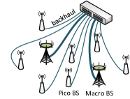
(a) Pico BSs with backhaul

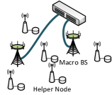
(b) Helper nodes with caches

Figure 1: Layouts of the considered two kinds of HetNets.

The distribution of MBSs, PBSs/helpers and users are modeled as three independent homogeneous PPPs, denoted as $\Phi_{1}$, $\Phi_{2}$ and $\Phi_{u}$ with density $\lambda_{1}$, $\lambda_{2}$ and $\lambda_{u}$, respectively. Each MBS is equipped with $M_{1}\geq 1$ antennas, and each PBS or helper node is equipped with $M_{2}=1$ antenna. The transmit power at each BS (or helper node) and pathloss exponent in the $k$th tier are $P_{k}$ and $\alpha_{k}$, respectively. Since the MBSs are able to connect to the core network via optical fiber with high capacity, while PBSs usually employ cost-effective DSL or microwave backhaul with low capacity, the backhaul capacity of each MBS is assumed as unlimited while the backhaul capacity of each PBS is assumed as a finite value, $C_{\rm bh}$.

We assume that each user randomly requests a file from a static content catalog that contains $N_{f}$ files. The files are indexed according to the popularity, ranking from the most popular (the 1${st}$ file) to the least popular (the $N_{f}$th file). The probability of requesting the $f$th file follows a Zipf-like distribution [15], i.e., $p_{f}={f^{-\delta}}\big{/}{\sum_{n=1}^{N_{f}}n^{-\delta}}$, where the skew parameter $\delta$ determines the “peakiness” of the distribution, whose typical value is between 0.5 and 1.0. For mathematical simplicity, we assume that the files are with unit size. Hence, the cache capacity of each helper node is $N_{c}$.

We assume that $\lambda_{u}\gg\lambda_{1}$ such that each MBS has at least $M_{1}$ users to serve. Since the density of PBSs (or helper nodes) may become comparable with the density of users along with the continuous network densification, some PBSs may have no users to serve. These inactive BSs will be turned into idle mode to avoid interference. Each MBS randomly selects $M_{1}$ users to serve at each time slot by zero-forcing beamforming (ZFBF) with equal power allocation, while each active PBS (or helper node) randomly selects one user to serve at each time slot with full power. These assumptions define a simple but typical scenario, which however can capture the basic elements and reflect fundamental tradeoffs.

Denote $k\in\{1,2\}$ as the index of the tier which a randomly chosen user (called the typical user) is associated with, and denote $r_{k}$ as the distance between the user and its associated BS $b_{k,0}$. The receive signal-to-interference-plus-noise ratio (SINR) of the typical user associated with BS $\!b_{k,0}$ is

$$\gamma_{k}\!=\!\frac{\frac{P_{k}}{M_{k}}h_{k,0}r_{k}^{-\alpha_{k}}}{\sum_{j=1}^{2}\sum_{i\in\tilde{\Phi}_{j}\backslash b_{k,0}}\!\!P_{j}h_{j,i}r_{j,i}^{-\alpha_{j}}+\sigma^{2}}\triangleq\frac{\frac{P_{k}}{M_{k}}h_{k,0}r_{k}^{-\alpha_{k}}}{I_{k}+\sigma^{2}}$$ (1)

where $r_{j,i}$ is the distance between the typical user and the $i$th active BS of the $j$th tier, $\tilde{\Phi}_{j}$ represents the set of active BSs in the $j$th tier, $h_{k,0}$ is the equivalent signal channel (including small-scale fading and precoding) from BS $b_{k,0}$ with unit mean, $h_{j,i}$ is the equivalent interference channel from the $i$th BS in the $j$th tier, and $\sigma^{2}$ is the noise power. We consider Rayleigh fading channels. Then, $h_{k,0}$ follows exponential distribution with unit mean (i.e., $h_{k,0}\sim\exp(1)$), and $h_{j,i}$ follows gamma distribution with shape parameter $M_{j}$ and unit mean (i.e., $h_{j,i}\sim\mathbb{G}(M_{j},\frac{1}{M_{j}})$) [16]. Note that the distribution of $h_{j,i}$ is very different from that assumed in [12, 13] for cache-enabled networks, where all the BSs have a single antenna. For notational simplicity, we define the interference power $I_{k}\triangleq\sum_{j=1}^{2}I_{k,j}\triangleq\sum_{i\in\tilde{\Phi}_{j}\backslash b_{k,0}}P_{j}h_{j,i}r_{j,i}^{-\alpha_{j}}$.

III ASE of Conventional HetNet

Consider that each user is associated with the BS with the strongest average receive power, say $P_{{\rm r},j}=P_{j}{r}_{j}^{-\alpha_{j}}$ for the BS in the $j$th tier. For notational brevity, we define the normalized transmit antenna number, transmit power and pathloss exponent of the $j$th tier when the typical user is associated with the $k$th tier as $\widehat{M}_{j}=\frac{M_{j}}{M_{k}}$, $\widehat{P}_{j}=\frac{P_{j}}{P_{k}}$, and $\widehat{\alpha}_{j}=\frac{\alpha_{j}}{\alpha_{k}}$, respectively. Note that $\widehat{M}_{k}=\widehat{P}_{k}=\widehat{\alpha}_{k}=1$.

For notational simplicity, the data rate of the typical user is expressed in unit of nats/s/Hz. The instantaneous achievable rate of a typical user associated with the macro tier is

$$R_{1}=\ln(1+\gamma_{1})$$ (2)

Different from the macro tier, the achievable rate of a typical user associated with the pico tier can not exceed the backhaul capacity, which is

$$R_{2}=\left\{\begin{array}[]{ll}\ln(1+\gamma_{2}),&\text{if}~{}\ln(1+\gamma_{2})\leq C_{\rm bh}\\ C_{\rm bh},&\text{if}~{}\ln(1+\gamma_{2})>C_{{\rm bh}}\end{array}\right.$$ (3)

In the sequel, we first derive the average achievable rate of the typical user associated with the pico tier, which is

$$\bar{R}_{2}=\mathbb{E}_{\gamma_{2},r_{2}}[R_{2}]=\int_{0}^{\infty}\mathbb{E}_{\gamma_{2}}[R_{2}|r]f_{r_{2}}(r)dr$$ (4)

where $\mathbb{E}_{\gamma_{2}}[R_{2}|r]$ is the conditional expectation of $R_{2}$ conditioned on $r_{2}=r$, $f_{r_{k}}(r)=\frac{2\pi\lambda_{k}}{\mathcal{P}_{k}}re^{-\pi\sum_{j=1}^{2}\lambda_{j}\widehat{P}_{j}{}^{{2}/{\alpha_{j}}}r^{{2}/{\widehat{\alpha}_{j}}}}$ is the probability density function (PDF) of the distance between the typical user and its serving BS, and $\mathcal{P}_{k}=2\pi\lambda_{k}\int_{0}^{\infty}re^{-\pi\sum_{j=1}^{2}\lambda_{j}\widehat{P}_{j}{}^{{2}/{\alpha_{j}}}r^{{2}/{\widehat{\alpha}_{j}}}}dr$ is the probability that the typical user is associated with the $k$th tier, which are given in Lemma 3 and Lemma 1 of [9], respectively.

Since $\mathbb{E}[X]=\int_{0}^{\infty}\mathbb{P}[X>x]dx$ for $X>0$ with $\mathbb{P}[\cdot]$ denoting probability, we obtain

$$\mathbb{E}_{\gamma_{2}}[R_{2}|r]\!=\!\!\int_{0}^{\infty}\mathbb{P}[R_{2}>x|r]dx\overset{(a)}{=}\!\!\int_{0}^{C_{\rm bh}}\mathbb{P}[\ln(1+\gamma_{2})>x|r]dx$$

$$\overset{(b)}{=}\int_{0}^{C_{\rm bh}}\mathbb{E}_{I_{2}}[\mathbb{P}[h_{2,0}>M_{2}P_{2}^{-1}r^{\alpha_{2}}(I_{2}+\sigma^{2})(e^{x}-1)|r,I_{2}]]dx$$

$$\overset{(c)}{=}\int_{0}^{C_{\rm bh}}\mathbb{E}_{I_{2}}[e^{-M_{2}P_{2}^{-1}r^{\alpha_{2}}(I_{2}+\sigma^{2})(e^{x}-1)}]dx$$

$$\overset{(d)}{=}\!\!\int_{0}^{C_{\rm bh}}\!e^{-\frac{M_{2}}{P_{2}}r^{\alpha_{2}}(e^{x}-1)\sigma^{2}}\!\prod_{j=1}^{2}\!\mathcal{L}_{I_{2,j}}\!\left(\tfrac{M_{2}}{P_{2}}r^{\alpha_{2}}(e^{x}-1)\right)dx$$ (5)

where step $(a)$ comes from the fact that $\mathbb{P}[R_{2}>C_{\rm bh}]=0$ due to (3), step $(b)$ is from (1) and using the law of total probability, step $(c)$ is from $h_{k0}\sim\exp(1)$, step $(d)$ follows because $\mathcal{L}_{\sum_{j}I_{k,j}}(s)=\prod_{i}\mathcal{L}_{I_{k,j}}(s)$, and $\mathcal{L}(\cdot)$ denotes the Laplace transform.

To derive the Laplace transform of $I_{k,j}$, we model the distribution of active BS $\tilde{\Phi}_{k}$ as a homogeneous PPP with density $p_{{\rm a},k}\lambda_{k}$ by thinning the BS distribution ${\Phi}_{k}$ as in [17], where $p_{{\rm a},k}$ is the probability that a BS in the $k$th tier is active, which can be derived as

$$p_{{\rm a},k}=1-\int_{0}^{\infty}e^{-\lambda_{u}x}f_{S_{k}}(x)dx\approx 1-\left(1+\tfrac{\mathcal{P}_{k}\lambda_{u}}{3.5\lambda_{k}}\right)^{-3.5}$$ (6)

where $f_{S_{k}}(x)$ is the PDF of the service area $S_{k}$ of a BS in the $k$th tier, and the approximation comes from $f_{S_{k}}(x)\approx\frac{3.5^{3.5}}{\Gamma(3.5)}\big{(}\tfrac{\lambda_{k}}{\mathcal{P}_{k}}\big{)}{}^{3.5}x^{2.5}e^{-3.5{\lambda_{k}x}/{\mathcal{P}_{k}}}$ in [18], which is exact when the HetNet degenerates into a homogeneous network. Note that for $k=1$ (i.e., the MBS tier), $p_{{\rm a},1}$ exactly equals to 1 since $\frac{\lambda_{u}}{\lambda_{1}}\to\infty$.

Proposition 1

The Laplace transform of the interference from the $j$th tier for a user associated with the $k$th tier is

$$\mathcal{L}_{I_{k,j}}(s)=\exp\Big{(}-\pi p_{{\rm a},j}\lambda_{j}\widehat{P}_{j}{}^{\frac{2}{\alpha_{j}}}r^{\frac{2}{\widehat{\alpha}_{j}}}\times\\ \big{(}{}_{2}F_{1}\big{[}-\tfrac{2}{\alpha_{j}},M_{j};1-\tfrac{2}{\alpha_{j}};-\tfrac{sP_{j}}{M_{j}\widehat{P}_{j}}r^{-\alpha_{k}}\big{]}-1\big{)}\Big{)}$$ (7)

where ${}_{2}F_{1}[\cdot]$ denotes the Gauss hypergeometric function.

Proof 1

See Appendix A.

With (7) and (5), the average rate in (4) becomes

$$\bar{R}_{2}=\frac{2\pi\lambda_{2}}{\mathcal{P}_{2}}\int_{0}^{\infty}\!\!\int_{0}^{C_{{\rm bh}}}\exp\bigg{(}-M_{2}P_{2}^{-1}r^{\alpha_{2}}(e^{x}-1)\sigma^{2}\\ -\pi\sum_{j=1}^{2}\lambda_{j}\widehat{P}_{j}{}^{\frac{2}{\alpha_{j}}}r^{\frac{2}{\widehat{\alpha}_{j}}}\big{(}1+p_{a,j}\mathcal{Z}_{j}(x)\big{)}\bigg{)}rdxdr$$ (8)

where $\mathcal{Z}_{j}(x)\triangleq{}_{2}F_{1}\big{[}-\tfrac{2}{\alpha_{j}},M_{j};1-\tfrac{2}{\alpha_{j}};\tfrac{(1-e^{x})}{\widehat{M}_{j}}\big{]}-1$.

By letting $C_{\rm bh}\to\infty$, the average achievable rate of a typical user associated with the macro tier can be similarly derived as

$$\bar{R}_{1}=\frac{2\pi\lambda_{1}}{\mathcal{P}_{1}}\int_{0}^{\infty}\!\!\int_{0}^{\infty}\!\exp\bigg{(}-M_{1}P_{1}^{-1}r^{\alpha_{1}}(e^{x}-1)\sigma^{2}\\ -\pi\sum_{j=1}^{2}\lambda_{j}\widehat{P}_{j}{}^{\frac{2}{\alpha_{j}}}r^{\frac{2}{\widehat{\alpha}_{j}}}(1+p_{a,j}\mathcal{Z}_{j}(x))\bigg{)}rdxdr$$ (9)

Since each active BS randomly selects $M_{k}$ users, the average throughput of a randomly chosen active cell in the $k$th tier is $M_{k}\bar{R}_{k}$. The ASE, defined as the average throughput of a network per unit area [19], can be obtained as

$${\rm ASE}=\sum_{j=1}^{2}p_{{\rm a},j}\lambda_{j}M_{j}\bar{R}_{j}$$ (10)

where $p_{{\rm a},j}\lambda_{j}$ is the density of active BSs in the $j$th tier.

Although $\bar{R}_{1}$ and $\bar{R}_{2}$ can be numerically computed from (9) and (8), the computational complexity is very high. In the following, we obtain closed-form expressions for approximated $\bar{R}_{1}$ and $\bar{R}_{2}$ in a special case, which are accurate even for the general cases as illustrated by simulations later.

III-A Special Case

Since HetNets are usually interference-limited, it is reasonable to neglect the thermal noise [9], i.e., $\sigma^{2}=0$. Furthermore, we consider equal path loss exponents of both tiers, $\alpha_{j}=\alpha$. Then, after a change of variables $r^{2}=v$, $\bar{R}_{2}$ in (8) can be further derived as

$$\bar{R}_{2}=\frac{\lambda_{2}}{\mathcal{P}_{2}}\int_{0}^{C_{{\rm bh}}}\bigg{(}\sum_{j=1}^{2}\lambda_{j}\widehat{P}_{j}{}^{\frac{2}{\alpha}}\big{(}1+p_{{\rm a},j}\mathcal{Z}_{j}(x)\big{)}\bigg{)}^{-1}dx$$ (11)

To derive a closed-form expression, we first obtain the approximation of $\mathcal{Z}_{j}(x)$ defined in (8). From the series-form expression ${}_{2}F_{1}[a,b;c;z]=\sum_{n=0}^{\infty}\frac{(a)_{n}(b)_{n}}{(c)_{n}}z^{n}$, where $(x)_{n}\triangleq x(x+1)\cdots(x+n-1)$ denotes the rising Pochhammer symbol, we can approximate $\mathcal{Z}_{j}(x)$ for small value of $x$ as

$$\mathcal{Z}_{j}(x) =\frac{2}{2-\alpha}\frac{M_{j}}{\widehat{M}_{j}}(1-e^{x})+\mathcal{O}\left((e^{x}-1)^{2}\right)$$

$$\overset{(a)}{=}\frac{2M_{k}}{\alpha-2}x+\mathcal{O}(x^{2})\approx\frac{2M_{k}}{\alpha-2}x\triangleq\mathcal{Z}_{j,low}(x)$$ (12)

where step (a) is from $1-e^{x}=x+\mathcal{O}(x^{2})$, and the approximation is accurate when $1-e^{x}\ll 1$, i.e., $x\ll\ln 2$. When the backhaul capacity is very stringent, i.e., $C_{\rm bh}\to 0$, by substituting (12) into (11) and then using $\mathcal{P}_{k}={\lambda_{k}}/{\sum_{j=1}^{2}\lambda_{j}\widehat{P}_{j}{}^{\frac{2}{\alpha}}}$ derived from Lemma 1 in [9], $\bar{R}_{2}$ can be approximated as

$$\bar{R}_{2}\approx \frac{\lambda_{2}}{\mathcal{P}_{2}}\int_{0}^{C_{{\rm bh}}}\bigg{(}\sum_{j=1}^{2}\lambda_{j}\widehat{P}_{j}{}^{\frac{2}{\alpha}}\big{(}1+p_{a,j}\mathcal{Z}_{j,low}(x)\big{)}\bigg{)}^{-1}dx$$

$$= \frac{\alpha-2}{2M_{2}}~{}\mathcal{C}_{1}\ln\left(1+\frac{2M_{2}}{\alpha-2}\cdot\frac{C_{\rm bh}}{\mathcal{C}_{1}}\right)$$ (13)

where $\mathcal{C}_{1}\triangleq\big{(}{\sum_{j=1}^{2}\lambda_{j}\widehat{P}_{j}{}^{\frac{2}{\alpha}}}\big{)}/\big{(}{\sum_{j=1}^{2}p_{{\rm a},j}\lambda_{j}\widehat{P}_{j}{}^{\frac{2}{\alpha}}}\big{)}$.

Similar as deriving (11), $\bar{R}_{1}$ in (9) can be derived as

$$\bar{R}_{1}=\frac{\lambda_{1}}{\mathcal{P}_{1}}\int_{0}^{\infty}\bigg{(}\sum_{j=1}^{2}\lambda_{j}\widehat{P}_{j}{}^{\frac{2}{\alpha}}\big{(}1+p_{{\rm a},j}\mathcal{Z}_{j}(x)\big{)}\bigg{)}^{-1}dx$$ (14)

By using the following transformation [20, eq. (9.132)],

$$\!\!\!\!\!{}_{2}F_{1}\left[a,b;c;z\right]=\tfrac{\Gamma(c)\Gamma(b-a)}{\Gamma(b)\Gamma(c-a)}(-z)^{-a}{}_{2}F_{1}\left[a,a\!+\!1\!-\!c;a+\!1\!-\!b;\tfrac{1}{z}\right]$$

$$~{}~{}~{}~{}~{}~{}+\tfrac{\Gamma(c)\Gamma(a-b)}{\Gamma(a)\Gamma(c-b)}(-z)^{-b}{}_{2}F_{1}\left[b,b\!+\!1\!-c;b+\!1\!-\!a;\tfrac{1}{z}\right]$$ (15)

and considering the series-form expression of ${}_{2}F_{1}[\cdot]$, we can approximate $\mathcal{Z}_{j}(x)$ for large value of $x$ as

$$\mathcal{Z}_{j}(x) =\tfrac{\Gamma\left(1-\frac{2}{\alpha}\right)\Gamma\left(M_{j}+\frac{2}{\alpha}\right)}{\Gamma(M_{j})}\big{(}\tfrac{e^{x}-1}{\widehat{M}_{j}}\big{)}^{\frac{2}{\alpha}}\!\!-1+\mathcal{O}\left((e^{x}-1)^{-M_{j}}\right)$$

$$\approx\tfrac{\Gamma\left(1-\frac{2}{\alpha}\right)\Gamma\left(M_{j}+\frac{2}{\alpha}\right)}{\Gamma(M_{j})\widehat{M}_{j}{}^{\frac{2}{\alpha}}}e^{\frac{2x}{\alpha}}-1\triangleq\mathcal{Z}_{j,high}(x)$$ (16)

where $\Gamma(x)$ is the Gamma function, and the approximation is accurate when $e^{x}-1\gg 1$, i.e., $x\gg\ln 2$.

By using the approximation $\mathcal{Z}_{j}(x)\approx\mathcal{Z}_{j,low}(x)$ for $x\in[0,\ln 2]$ and $\mathcal{Z}_{j}(x)\approx\mathcal{Z}_{j,high}(x)$ for $x\in[\ln 2,\infty)$, we can approximate $\bar{R}_{1}$ as

$$\bar{R}_{1} \approx\frac{\lambda_{1}}{\mathcal{P}_{1}}\int_{0}^{\ln 2}\bigg{(}\sum_{j=1}^{2}\lambda_{j}\widehat{P}_{j}^{\frac{2}{\alpha}}\left(1+p_{a,j}\mathcal{Z}_{j,low}(x)\right)\bigg{)}^{-1}dx$$

$$~{}~{}~{}+\frac{\lambda_{1}}{\mathcal{P}_{1}}\int_{\ln 2}^{\infty}\bigg{(}\sum_{j=1}^{2}\lambda_{j}\widehat{P}_{j}^{\frac{2}{\alpha}}\left(1+p_{{\rm a},j}\mathcal{Z}_{j,high}(x)\right)\bigg{)}^{-1}dx$$

$$=\frac{\alpha-2}{2M_{1}}\mathcal{C}_{1}\ln\left(1+\frac{2M_{1}}{\alpha-2}\!\cdot\!\frac{\ln 2}{\mathcal{C}_{1}}\right)+\frac{\alpha}{2}\mathcal{C}_{2}\ln\big{(}1+\mathcal{C}_{3}4^{-\frac{1}{\alpha}}\big{)}$$ (17)

where $\mathcal{C}_{2}\triangleq\big{(}\sum_{j=1}^{2}\lambda_{j}\widehat{P}_{j}{}^{\frac{2}{\alpha}}\big{)}/\big{(}\sum_{j=1}^{2}(1-p_{{\rm a},j})\lambda_{j}\widehat{P}_{j}{}^{\frac{2}{\alpha}}\big{)}$, $\mathcal{C}_{3}\triangleq\big{(}\sum_{j=1}^{2}(1-p_{{\rm a},j})\lambda_{j}\widehat{P}_{j}{}^{\frac{2}{\alpha}}\big{)}/\big{(}\sum_{j=1}^{2}p_{{\rm a},j}\lambda_{j}\widehat{P}_{j}{}^{\frac{2}{\alpha}}\mathcal{M}_{j}\big{)}$, and $\mathcal{M}_{j}\triangleq{\Gamma(1-\frac{2}{\alpha})\Gamma(M_{j}+\frac{2}{\alpha})}/\big{(}{\Gamma(M_{j})\widehat{M}_{j}{}^{\frac{2}{\alpha}}}\big{)}$.

By substituting (17) and (13) into (10), we can obtain the closed-form expression of an approximated ASE, which is accurate as shown by simulation later.

IV ASE of Cache-enabled HetNet

We consider that each helper node caches the $N_{c}$ most popular files, which is the optimal caching policy in terms of cache hit-ratio when each user can only associate with one node [5].

We call a user whose requested file is cached at the helper node as a cache-hit user and the others as cache-miss users. The probability that the typical user is a cache-hit user is

$$p_{\rm h}=\sum_{f=1}^{N_{c}}p_{f}=\frac{\sum_{f=1}^{N_{c}}f^{-\delta}}{\sum_{n=1}^{N_{f}}n^{-\delta}}$$ (18)

Since the users are distributed as PPP and the file requests of the users are independent and identical, the distribution of cache-hit users and cache-miss users also follow PPPs, respectively with density $p_{\rm h}\lambda_{u}$ and $(1-p_{\rm h})\lambda_{u}$.

Considering that helpers are not connected with backhaul, cache-miss users can only associate with the macro tier, while cache-hit users can associate either with macro or helper tier.

For the cache-hit users, the cell association is based on the maximal average receive power. Then, the probability that a cache-hit user is associated with the $k$th tier can be obtained from Lemma 1 in [9] as

$$\mathcal{P}_{{\rm h},k}=2\pi\lambda_{k}\int_{0}^{\infty}re^{-\pi\sum_{j=1}^{2}\lambda_{j}\widehat{P}_{j}{}^{2/\alpha_{j}}r^{2/\widehat{\alpha}_{j}}}dr$$ (19)

Since the cache-miss users can only associate with the macro tier, the tier association probability is $\mathcal{P}_{{\rm m},k}=1$ for $k=1$ and $\mathcal{P}_{{\rm m},k}=0$ for $k=2$.

From the law of total probability, the probability that the typical user is associated with a MBS or a helper is

$$\mathcal{P}_{1} =p_{\rm h}\mathcal{P}_{{\rm h},1}+(1-p_{\rm h})\mathcal{P}_{{\rm m},1}=p_{\rm h}\mathcal{P}_{{\rm h},1}+1-p_{\rm h}$$ (20)

$$\mathcal{P}_{2} =p_{\rm h}\mathcal{P}_{{\rm h},2}+(1-p_{\rm h})\mathcal{P}_{{\rm m},2}=p_{\rm h}\mathcal{P}_{{\rm h},2}$$ (21)

From (20) and using the conditional probability formula, we can also obtain the probability that a typical user associated with the MBS is a cache-hit user as $p_{1,{\rm h}}={p_{\rm h}\mathcal{P}_{{\rm h},1}}/{\mathcal{P}_{1}}$, which is essential for the following derivation.

Similar to the conventional HetNet, the probability that a BS in the $k$th tier is active is $p_{{\rm a},k}\approx 1-\big{(}1+\tfrac{\mathcal{P}_{k}\lambda_{u}}{3.5\lambda_{k}}\big{)}^{-3.5}$.

Considering that the cell association of cache-hit users is based on maximal average receive power (the same as in conventional HetNet), the average achievable rate of the typical cache-hit user associated with the $k$th tier can be obtained similarly as we deriving (9), which is

$$\bar{R}_{{\rm h},k}=\frac{2\pi\lambda_{k}}{\mathcal{P}_{{\rm h},k}}\int_{0}^{\infty}\!\!\int_{0}^{\infty}\!\!\exp\bigg{(}-M_{k}P_{k}^{-1}r^{\alpha_{k}}(e^{x}-1)\sigma^{2}\\ -\pi\sum_{j=1}^{2}\lambda_{j}\widehat{P}_{j}{}^{\frac{2}{\alpha_{j}}}r^{\frac{2}{\widehat{\alpha}_{j}}}(1+p_{a,j}\mathcal{Z}_{j}(x))\bigg{)}rdxdr$$ (22)

Different from the conventional pico tier, when a cache-hit user is associated with a helper, the helper node can fetch the requested file from its local cache, hence the achievable rate is no longer limited by the backhaul capacity.

Since cache-miss users can only associate with the macro tier, the PDF of the distance between a typical cache-miss user and its serving MBS is [10]

$$f_{r_{1}}(r)=2\pi\lambda_{1}re^{-\lambda_{1}\pi r^{2}}$$ (23)

Similar to the derivation of (4) and (5), we can obtain the average achievable rate of the typical cache-miss user as

$$\bar{R}_{m}\!\!=\!\!\int\limits_{0}^{\infty}\!\int\limits_{0}^{\infty}\!\!f_{r_{1}}\!(r)e^{-\frac{M_{1}}{P_{1}}r^{\alpha_{1}}\!(e^{x}\!-1)\sigma^{2}}\!\prod\limits_{j=1}^{2}\!\mathcal{L}_{I_{1,j}}\!\big{(}\tfrac{M_{1}}{P_{1}}r^{\alpha_{1}}\!(e^{x}\!-1)\big{)}dxdr$$

where $\mathcal{L}_{I_{1,j}}$ is given in the following proposition.

Proposition 2

The Laplace transform of the interference from the $j$th tier when the typical cache-miss user is associated with the macro tier, $\mathcal{L}_{I_{1,j}}(s)$, is

$$\left\{\begin{array}[]{ll}\!\!e^{-\pi p_{{\rm a},1}\lambda_{1}r^{2}\big{(}\!{}_{2}F_{1}\big{[}-\frac{2}{\alpha_{1}},M_{1};1-\frac{2}{\alpha_{2}};-\frac{sP_{1}}{M_{1}}r^{-\alpha_{1}}\!\big{]}\!-1\big{)}},&\!\!\!\!\!j=1\\ \!\!e^{-\pi p_{{\rm a},2}\lambda_{2}{\Gamma(1-\frac{2}{\alpha_{2}})\Gamma(M_{2}+\frac{2}{\alpha_{2}}\!)}{\Gamma(M_{2})}^{-1}\big{(}\frac{sP_{2}}{M_{2}}\big{)}^{\frac{2}{\alpha_{2}}}},&\!\!\!\!\!j=2\end{array}\right.$$ (24)

Proof 2

See Appendix B

Substituting (24) and (23) into (5) and setting $C_{\rm bh}\to\infty$, we obtain the average achievable rate of the typical cache-miss user as,

$$\bar{R}_{\rm m}=2\pi\lambda_{1}\int_{0}^{\infty}\!\!\int_{0}^{\infty}\!\exp\Big{(}-M_{1}P_{1}^{-1}r^{\alpha_{1}}(e^{x}-1)\sigma^{2}$$

$$-\pi\lambda_{1}r^{2}\left(1+p_{{\rm a},1}\mathcal{Z}_{1}(x)\right)-\pi\lambda_{2}r^{\frac{2}{\widehat{\alpha}_{2}}}\widehat{P}_{2}{}^{\frac{2}{\alpha_{2}}}p_{{\rm a},2}\times$$

$$~{}{\Gamma\big{(}1-\tfrac{2}{\alpha_{2}}\big{)}\Gamma\big{(}M_{2}+\tfrac{2}{\alpha_{2}}\big{)}}{\Gamma(M_{2})}^{-1}\widehat{M}_{2}{}^{-\frac{2}{\alpha_{2}}}(e^{x}-1)^{\frac{2}{\alpha_{2}}}\Big{)}rdxdr$$ (25)

where $\mathcal{Z}_{1}(x)$ is defined in (8).

According to the law of total probability, the average cell throughput of a randomly chosen active MBS is

$$\bar{R}_{1}=\sum_{n_{\rm h}=0}^{M_{1}}p_{n_{\rm h}}(n_{\rm h}\bar{R}_{{\rm h,1}}+(M_{1}-n_{\rm h})\bar{R}_{m})$$ (26)

where $p_{n_{\rm h}}=\binom{M_{1}}{n_{\rm h}}p_{1,\rm h}^{k}(1-p_{1,{\rm h}})^{M_{1}-k}$ is the probability that $n_{k}$ users among the $M_{1}$ random scheduled users are cache-hit users, and $p_{1,{\rm h}}$ is given after (20), $n_{\rm h}\bar{R}_{{\rm h,1}}+(M_{1}-n_{\rm h})\bar{R}_{m}$ is the average throughput of each macro cell conditioned on that $n_{k}$ users among the $M_{1}$ users are cache-hit users.

Since the helper tier can only serve cache-hit users, the average cell throughput of a randomly chosen active helper is $\bar{R}_{2}=\bar{R}_{\rm h,2}$. Then, the ASE of the network can be obtained as

$${\rm ASE}=\sum_{j=1}^{2}p_{{\rm a},j}\lambda_{j}\bar{R}_{j}$$ (27)

In the following, we derive closed-form expressions for approximated $\bar{R}_{{\rm h},k}$ and $\bar{R}_{\rm m}$ in a special case.

IV-A Special Case

Again, by neglecting thermal noise and considering equal path loss for both tiers, similar to the derivation of $\eqref{eqn:cER1}$, the average achievable rate of the typical cache-hit user can be approximated as

$$\bar{R}_{{\rm h},k}\approx\frac{\alpha-2}{2M_{k}}\mathcal{C}_{1}\!\ln\left(\!1+\frac{2M_{k}}{\alpha-2}\!\cdot\!\frac{\ln 2}{\mathcal{C}_{1}}\right)+\frac{\alpha}{2}\mathcal{C}_{2}\ln\big{(}1+\mathcal{C}_{3}4^{-\frac{1}{\alpha}}\big{)}$$ (28)

where $\mathcal{C}_{1}$ is given in (13), $\mathcal{C}_{2}$ and $\mathcal{C}_{3}$ are given in (17).

Considering $\sigma^{2}=0$, $\alpha_{j}=\alpha$ and with a change of variables $r^{2}=v$ in (25), $\bar{R}_{\rm m}$ can be derived as

$$\bar{R}_{\rm m}=\lambda_{1}\int_{0}^{\infty}\!\Big{(}\lambda_{1}\left(1+p_{{\rm a},1}\mathcal{Z}_{1}(x)\right)+\lambda_{2}\widehat{P}_{2}{}^{\frac{2}{\alpha}}p_{{\rm a},2}\times\\ {\Gamma\big{(}1-\tfrac{2}{\alpha_{2}}\big{)}\Gamma\big{(}M_{2}+\tfrac{2}{\alpha_{2}}\big{)}}{\Gamma(M_{2})}^{-1}\widehat{M}_{2}^{-\frac{2}{\alpha_{2}}}(e^{x}-1)^{\frac{2}{\alpha_{2}}}\Big{)}^{-1}dx$$ (29)

Considering that $\mathcal{Z}_{j}(x)$ can be approximated as $\mathcal{Z}_{j,low}(x)$ given in (12) for $x\in[0,\ln 2]$ and as $\mathcal{Z}_{j,high}(x)$ given in (16) for $x\in[\ln 2,\infty)$, the average achievable rate of the typical cache-miss user can be approximated as

$$\bar{R}_{\rm m} \approx\lambda_{1}\int_{0}^{\ln 2}\!\big{(}\lambda_{1}(1+p_{{\rm a},1}\mathcal{Z}_{1,low})\big{)}^{-1}dx$$

$$~{}~{}~{}+\lambda_{1}\int_{\ln 2}^{\infty}\bigg{(}\sum_{j=1}^{2}\lambda_{j}\widehat{P}_{j}{}^{\frac{2}{\alpha}}\left(1+p_{{\rm a},j}\mathcal{Z}_{j,high}(x)\right)\bigg{)}^{-1}dx$$

$$=\!\frac{\alpha-2}{2p_{\rm a,1}M_{1}}\ln\left(1\!+\frac{2p_{\rm a,1}M_{1}}{\alpha-2}\!\ln 2\right)+\frac{\alpha}{2}\mathcal{C}_{4}\!\ln\!\big{(}1\!+\mathcal{C}_{3}4^{-\frac{1}{\alpha}}\big{)}$$ (30)

where we also use the approximation $e^{x}-1=\mathcal{O}(x)\approx 0$ for $x\in[0,\ln 2]$ and $e^{x}-1\approx e^{x}$ for $x\in[\ln 2,\infty)$, and $\mathcal{C}_{4}\triangleq 1/\big{(}\sum_{j=1}^{2}(1-p_{{\rm a},j})\lambda_{j}\widehat{P}_{j}{}^{\frac{2}{\alpha}}\big{)}$.

By substituting (28) and (30) into (27), we can obtain the closed-form expression of an approximated ASE, which is accurate as shown by simulation later.

V Numerical and Simulation Results

In this section, we validate the analytical results via simulations and compare the performance of conventional and cache-enabled HetNets by numerical results.

The simulation parameters are given in Table I. To reflect the impact of the file catalog size, we use normalized cache capacity $\eta=\frac{N_{c}}{N_{f}}$ in the following.

TABLE I: Simulation parameters

Parameters	Value
MBS density, $\lambda_{1}$	$1/(500^{2}\pi)$ m-2 [9]
User density, $\lambda_{u}$	$50/(500^{2}\pi)$ m-2
Path loss exponent, $\alpha$	3.7
Transmit power of each MBS, $P_{1}$	46 dBm
Transmit power of each PBSs/helper node, $P_{2}$	21 dBm
Number of antennas at each MBS, $M_{1}$	4
Transmission bandwidth, $W$	20 MHz
File catalog size, $N_{f}$	$10^{5}$ files [5]
Zipf-like distribution skew parameter, $\delta$	0.8 [4]

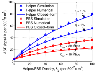
(a) ASE v.s. helper/PBS density $\lambda_{2}$.

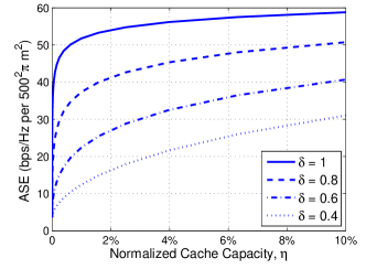
(b) ASE v.s. $\eta$, $\lambda_{2}=50/(500^{2}\pi)$.

Figure 2: ASE v.s. helper/PBS density and normalized cache capacity.

In Fig. 2(a), we compare the ASE of the two HetNets, where the numerical results are obtained from substituting (8) and (9) into (10) for conventional HetNet and substituting (22) and (25) into (27) with (26) for cache-enabled HetNet, the results of the closed-form expression are obtained from substituting (13) and (17) into (10) for conventional HetNet and substituting (28) and (30) into (27) with (26) for cache-enabled HetNet. We can see that the results obtained from closed-form expressions are very close to the numerical and simulation results. In fact, same conclusion can be obtained from the simulation results using typical values of $\alpha_{j}$ for different tiers, which are not shown for conciseness. Note that in the simulation, $\sigma^{2}\neq 0$. These indicate that the approximations are very accurate even without the assumption of $\sigma^{2}=0$, $\alpha_{j}=\alpha$. Hence, in the sequel we only provide the analytical results obtained from the closed-form expressions. Compared with the conventional HetNet with limited-capacity backhaul (e.g., $C_{\rm bh}=10$ Mbps), the cache-enabled HetNet can double the ASE when each helper node only caches 1% of the total files. Alternatively, to achieve the same ASE, the helper node density is much lower than the PBS density, which can reduce the deploying and operating cost remarkably (e.g., when $C_{\rm bh}=10$ Mbps and $\eta=1\%$, the helper node density is about 1/4 of the PBS density to achieve an ASE of $20/(500^{2}\pi)$ bps/Hz/m²). As expected, the ASE of cache-enabled HetNet increases with $\eta$. Furthermore, when $\delta$ is larger, the ASE grows with $\eta$ more rapidly for small value of $\eta$ and grows with $\eta$ more slowly for large $\eta$.

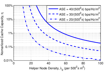
Figure 3: Trade-off between helper density and cache capacity.

Since the ASE of cache-enabled HetNet can be improved either by increasing cache capacity or increasing helper density, a natural question is that how much helper density can be traded off by cache capacity to achieve a target ASE? To answer this question, we set the ASE as different values and show the normalized cache capacity versus helper density in Fig. 3. With a given target ASE and helper density, $\eta$ can be found by substituting (18), (26) into (27) and then using the bisection search method. It is shown that we can reduce the helper density by increasing the cache capacity of each helper. For example, to achieve a target ASE of $20/(500^{2}\pi)$ bps/Hz/m², by increasing the cache capacity from $\eta=0.01\%$ to $\eta=0.1\%$, the helper density can be reduced by two thirds. Similar trade-off between BS density and cache capacity was reported in [11], where a homogeneous network with single antenna BSs was considered and the performance metric was outage probability. In our work, the helper density can be traded off more significantly by the cache capacity.

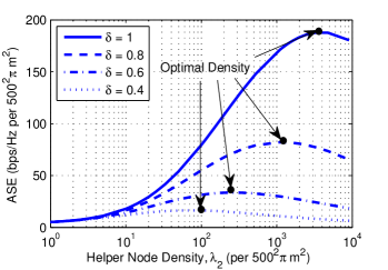
Figure 4: ASE v.s. helper density with given $\lambda_{2}N_{c}=10^{4}/(500^{2}\pi)$.

Inspired by such a trade-off, another natural question is: with a given total amount of cache capacity within an area, should we deploy the caches in a distributed manner (i.e., more helpers each with less cache capacity) or in a centralized manner (i.e., less helpers each with more cache capacity) in order to maximize the ASE? To answer this question, we fix the area cache capacity $\lambda_{2}N_{c}$ as a constant and provide the ASE versus the helper density in Fig. 4. We can see that there exists an optimal helper density maximizing the ASE. Moreover, the optimal density increases with $\delta$, which means that the more skewed the file popularity is, the more distributedly we should deploy the caches. This can be explained from the impact of the following two observations in Figs. 2(a) and 2(b). On one hand, with given cache capacity of each helper, the ASE increases with the helper density first rapidly and then slowly. On the other hand, with given helper density, the ASE reduces with the decrease of cache capacity first slowly and then rapidly, and the larger $\delta$ is, the more slowly the ASE decreases with $\eta$ when the cache capacity is large.

VI Conclusion

In this paper, we investigated the gain of cache-enabled HetNet over conventional HetNet with limited capacity backhaul, and addressed the tradeoff in deploying the cache-enabled HetNet. We obtained closed-form expressions of the approximated ASEs of these two HetNets. We then used numerical results to show that cache-enabled HetNet can double the ASE over conventional HetNet with the same BS/helper density. To achieve the same ASE, the helper density is much lower than the PBS density and can be traded off by cache capacity. For a given total cache capacity within an area, there exists an optimal helper density maximizing the ASE.

Appendix A Proof of Proposition 1

The Laplace transform of $I_{k,j}$ can be derived as

$$\mathcal{L}_{I_{k,j}}(s)=\mathbb{E}_{\tilde{\Phi}_{j},h_{j,i}}\left[e^{-s\sum_{i\in\tilde{\Phi}_{j}}P_{j}h_{j,i}r_{j,i}^{-\alpha_{j}}}\right]$$

$$\overset{(a)}{=}\mathbb{E}_{\tilde{\Phi}_{j}}\left[\prod_{i\in\tilde{\Phi}_{j}}\left(1+\frac{sP_{j}}{M_{j}}r_{j,i}^{-\alpha_{j}}\right)^{-M_{j}}\right]$$

$$\overset{(b)}{=}\exp\left(-2\pi p_{{\rm a},j}\lambda_{j}\int_{r_{0,j}}^{\infty}\left(1-\left({1+\frac{sP_{j}}{M_{j}}u^{-\alpha_{j}}}\right)^{-M_{j}}\right)udu\right)$$

$$\overset{(c)}{=}\exp\left(\!-\pi p_{{\rm a},j}\lambda_{j}\int_{r_{0,j}^{2}}^{\infty}\left(1-\left(1+\frac{sP_{j}}{M_{j}}v^{-\frac{\alpha_{j}}{2}}\right)^{-M_{j}}\right)dv\right)$$ (31)

where step $(a)$ follows from $h_{j,i}\sim\mathbb{G}(M_{j},\frac{1}{M_{j}})$, step $(b)$ follows from the probability generating function of the PPP, and step $(c)$ is obtained by changing variables as $u^{2}=v$.

To derive the integration in (31), we first obtain the indefinite integration as

$$\int\left(1-\left(1+\frac{sP_{j}}{M_{j}}v^{-\frac{\alpha_{j}}{2}}\right)^{-M_{j}}\right)dv$$

$$\overset{(a)}{=}\int dv-\int\sum_{n=0}^{\infty}\frac{(-1)^{n}(M_{j})_{n}}{n!}\left(\frac{sP_{j}}{M_{j}}v^{-\frac{\alpha_{j}}{2}}\right)^{n}dv$$

$$=v-\sum_{n=0}^{\infty}\frac{(-1)^{n}(M_{j})_{n}}{n!}\int\left(\frac{sP_{j}}{M_{j}}v^{-\frac{\alpha_{j}}{2}}\right)^{n}dv$$

$$=v-v\sum_{n=0}^{\infty}\frac{(-\frac{2}{\alpha_{j}})_{n}(M_{j})_{n}}{(1-\frac{2}{\alpha_{j}})_{n}}\frac{\left(-\frac{sP_{j}}{M_{j}}v^{-\frac{\alpha_{j}}{2}}\right)^{n}}{n!}$$

$$\overset{(b)}{=}v\big{(}1-{}_{2}F_{1}\big{[}-\tfrac{2}{\alpha_{j}},M_{j};1-\tfrac{2}{\alpha_{j}};-\tfrac{sP_{j}}{M_{j}}v^{-\frac{\alpha_{j}}{2}}\big{]}\big{)}$$ (32)

where step (a) is from the generalized binomial theorem, $(x)_{n}\triangleq x(x+1)\cdots(x+n-1)$ denotes the rising Pochhammer symbol, step (b) is from the series-form expression of Gauss hypergeometric function ${}_{2}F_{1}[\cdot]$.

By introducing the integration limits and after some manipulations, we obtain

$$\int_{r_{0,j}^{2}}^{\infty}\left(1-\left(1+\frac{sP_{j}}{M_{j}}v^{-\frac{\alpha_{j}}{2}}\right)^{-M_{j}}\right)dv\\ =r_{0,j}^{2}\big{(}{}_{2}F_{1}\big{[}-\tfrac{2}{\alpha_{j}},M_{j};1-\tfrac{2}{\alpha_{j}};-\tfrac{sP_{j}}{M_{j}}r_{0,j}^{-\alpha_{j}}\big{]}-1\big{)}$$ (33)

The lower limit of the integration is $r_{0,j}=\widehat{P}_{j}{}^{\frac{1}{\alpha_{j}}}r^{\frac{1}{\widehat{\alpha}_{j}}}$, which is the possibly closest distance of the interfering BS in the $j$th tier. By considering the integration limit $r_{0,j}$ and substituting (33) into (31), the proposition can be proved.

Appendix B Proof of Proposition B

Similar to the derivation of (7), we obtain

$$\mathcal{L}_{I_{1,j}}(s)\!=e^{\!-\pi p_{{\rm a},j}\lambda_{j}r_{0,j}^{2}\big{(}\!{}_{2}F_{1}\big{[}-\frac{2}{\alpha_{j}},M_{j};1-\frac{2}{\alpha_{j}};-\frac{sP_{j}}{M_{j}}r^{-\alpha_{j}}\!\big{]}\!-\!1\big{)}}$$ (34)

where $r_{0,j}=r$ for $j=1$ and $r_{0,j}\to 0$ for $j=2$ (helper tier). The proposition can be proved by substituting $r_{0,j}$ and considering $\lim_{r_{0,j}\to 0}r_{0,j}^{2}\big{(}{}_{2}F_{1}\big{[}-\tfrac{2}{\alpha_{j}},M_{j};1-\tfrac{2}{\alpha_{j}};-\tfrac{sP_{j}}{M_{j}}r_{0,j}^{-\alpha_{j}}\big{]}-1\big{)}={\Gamma\big{(}1-\frac{2}{\alpha_{j}}\big{)}\Gamma\big{(}M_{1}+\frac{2}{\alpha_{j}}\big{)}}{\Gamma(M_{j})}^{-1}\big{(}\frac{sP_{j}}{M_{j}}\big{)}^{\frac{2}{\alpha_{j}}}$ derived from (15).

References

• [1] N. Bhushan et al., “Network densification: the dominant theme for wireless evolution into 5G,” IEEE Commun. Mag., vol. 52, no. 2, pp. 82–89, Feb. 2014.
• [2] A. Ghosh et al., “Heterogeneous cellular networks: From theory to practice,” IEEE Commun. Mag., vol. 50, no. 6, pp. 54–64, Jun. 2012.
• [3] V. Chandrasekhar, J. Andrews, and A. Gatherer, “Femtocell networks: a survey,” IEEE Commun. Mag., vol. 46, no. 9, pp. 59–67, Sept. 2008.
• [4] S. Woo et al., “Comparison of caching strategies in modern cellular backhaul networks,” in Proc. ACM MobiSys, 2013.
• [5] N. Golrezaei, K. Shanmugam, A. G. Dimakis, A. F. Molisch, and G. Caire, “Femtocaching: Wireless video content delivery through distributed caching helpers,” in Proc. IEEE INFOCOM, 2012.
• [6] E. Bastug, M. Bennis, and M. Debbah, “Living on the edge: The role of proactive caching in 5G wireless networks,” IEEE Commun. Mag., vol. 52, no. 8, pp. 82–89, Aug. 2014.
• [7] D. Liu and C. Yang, “Will caching at base station improve energy efficiency of downlink transmission?” in Proc. IEEE GlobalSIP, 2014.
• [8] ——, “Energy efficiency of downlink networks with caching at base stations,” IEEE J. Sel. Areas Commun., to appear.
• [9] H.-S. Jo, Y. J. Sang, P. Xia, and J. Andrews, “Heterogeneous cellular networks with flexible cell association: A comprehensive downlink sinr analysis,” IEEE Trans. Wireless Commun., vol. 11, no. 10, pp. 3484–3495, Oct. 2012.
• [10] J. Andrews, F. Baccelli, and R. Ganti, “A tractable approach to coverage and rate in cellular networks,” IEEE Trans. Commun., vol. 59, no. 11, pp. 3122–3134, Nov. 2011.
• [11] E. Bastug, M. Bennis, M. Kountouris, and M. Debbah, “Cache-enabled small cell networks: modeling and tradeoffs,” EURASIP J. on Wireless Commun. and Netw., vol. 2015, no. 1, 2015.
• [12] C. Yang, Z. Chen, Y. Yao, and B. Xia, “Performance analysis of wireless heterogeneous networks with pushing and caching,” in Proc. IEEE ICC, 2015.
• [13] S. H. Chae, J. Y. Ryu, T. Q. S. Quek, and W. Choi, “Cooperative transmission via caching helpers,” in Proc. IEEE GLOBECOM, 2015.
• [14] N. Golrezaei, A. F. Molisch, A. G. Dimakis, and G. Caire, “Femtocaching and device-to-device collaboration: A new architecture for wireless video distribution,” IEEE Commun. Mag., vol. 51, no. 4, pp. 142–149, Apr. 2013.
• [15] L. Breslau, P. Cao, L. Fan, G. Phillips, and S. Shenker, “Web caching and Zipf-like distributions: Evidence and implications,” in Proc. IEEE INFOCOM, 1999.
• [16] N. Jindal, J. Andrews, and S. Weber, “Multi-antenna communication in ad hoc networks: Achieving MIMO gains with SIMO transmission,” IEEE Trans. Commun., vol. 59, no. 2, pp. 529–540, Feb. 2011.
• [17] S. Lee and K. Huang, “Coverage and economy of cellular networks with many base stations,” IEEE Commun. Lett., vol. 16, no. 7, pp. 1038–1040, July 2012.
• [18] S. Singh, H. Dhillon, and J. Andrews, “Offloading in heterogeneous networks: Modeling, analysis, and design insights,” IEEE Trans. Wireless Commun., vol. 12, no. 5, pp. 2484–2497, May 2013.
• [19] Y. S. Soh, T. Quek, M. Kountouris, and H. Shin, “Energy efficient heterogeneous cellular networks,” IEEE J. Sel. Areas Commun., vol. 31, no. 5, pp. 840–850, May 2013.
• [20] A. Jeffrey and D. Zwillinger, Table of integrals, series, and products, 6th ed.   Academic Press, 2000.