Random numbers from vacuum fluctuations

Abstract

We implement a quantum random number generator based on a balanced homodyne measurement of vacuum fluctuations of the electromagnetic field. The digitized signal is directly processed with a fast randomness extraction scheme based on a linear feedback shift register. The random bit stream is continuously read in a computer at a rate of about 480 Mbit/s and passes an extended test suite for random numbers.

I Introduction

Various cryptographic schemes, classical or quantum, require high quality and trusted random numbers for key generation and other aspects of the protocols. In order to keep up with data rates in modern communication schemes, these random numbers need to be generated at a high rate Gisin et al. (2002). Equally, large amounts of random numbers are at the core of Monte Carlo simulation methods Metropolis (1987). Algorithmically generated pseudo-random numbers are available at very high rates, but are deterministic by definition and are unsuitable for cryptographic purposes, as they may contain backdoors in the particular algorithm used to generate them. For applications that require unpredictable random numbers, physical random number generators (PRNG) have been used in the past Galton (1890) and more recently Jun and Kocher (1999). These involve measuring noisy physical processes and conversion of the outcome into random numbers. Since it is either practically (e.g. for thermal noise sources) or fundamentally (for certain quantum processes) impossible to predict the outcome of such measurements, these physically generated random numbers are considered “truly” random.

Quantum random number generators (QRNG) belong to a class of physical random number sources where the source of randomness is the fundamentally unpredictable outcome of a quantum measurement. Early PRNG of this class were based on observing the decay statistics of radioactive nuclei Gude (1985); Figotin et al. (2004). More recently, similar PRNG based on Poisson statistics in optical photon detection were implemented Stipcevic and Rogina (2007); Wayne et al. (2009); Fürst et al. (2010); Wayne and Kwiat (2010); Wahl et al. (2011). Different schemes use the randomness of a single photon scattered by a beam splitter into either of two output ports Jennewein et al. (2000); Stefanov et al. (2000). Since the reflection/transmission of the photon is intrinsically random due to the quantum nature of the process, the unpredictability of the generated numbers is ensured Frauchiger and Renner (2013). Other implementations of QRNGs measure the amplified spontaneous emission Williams et al. (2010), the vacuum fluctuations of the electromagnetic field Gabriel et al. (2010); Symul, Assad, and Lam (2011); Shen, Tian, and Zou (2010), or the intensity Kanter et al. (2009); Sanguinetti et al. (2014) and phase noise of different light sources Qi et al. (2010); Xu et al. (2012); Abellán et al. (2014, 2015); Yuan et al. (2014).

In this paper we report on a quantum random number generator based on measuring vacuum fluctuations as the raw source of ramdomness Gabriel et al. (2010); Symul, Assad, and Lam (2011); Shen, Tian, and Zou (2010). Such measurements have a very high bandwidth compared to schemes based on photon counting Stipcevic and Rogina (2007); Fürst et al. (2010), and have a much simpler optical setup compared to phase noise measurements Qi et al. (2010); Xu et al. (2012); Abellán et al. (2014, 2015); Yuan et al. (2014). Coupled with an efficient randomness extractor, we obtain an unbiased, uncorrelated stream of random bits at high speed.

II Implementation

Figure 1 schematically shows the setup of our QRNG. A continuous wave laser (wavelength 780 nm) is used as the local oscillator (LO) for the vacuum fluctuations of the electromagnetic field entering the beam splitter at the empty port. The output of the beam splitter is directed onto two pin photodiodes, and the photocurrent difference is processed further.

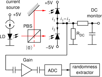
Figure 1: Schematic of the quantum random number generator. A polarizing beam splitter (PBS) distributes the light of a 780 nm laser diode equally onto two fast photodiodes, generating photocurrents $i_{1}$ and $i_{2}$. The fluctuations in the photocurrent difference $i_{1}-i_{2}$ are amplified, digitized, and sent to a randomness extractor to generate unbiased “true” random numbers.

This setup is known as a balanced homodyne detector Jakeman, Oliver, and Pike (1975); Yuen and Chan (1983) and maps the the electrical field in the second mode entering the beam splitter to the photocurrent difference $i_{1}-i_{2}$. Here, the second input port is empty, so the homodyne measurement is probing the vacuum state of the electromagnetic field. This field fluctuates Glauber (1963), and is used as the source of randomness. As the vacuum field is independent of external physical quantities, it can not be tampered with. Since the optical power impinging on the two photodiodes is balanced, any power fluctuation in the local oscillator will be simultaneously detected by the two diodes, and therefore cancel in the photocurrent difference Yuen and Chan (1983); Schumaker (1984). In an alternative view, the laser beam can be seen as generating photocurrents $i_{1},i_{2}$ with a shot noise power proportional to the average optical power. The shot noise currents from the two diodes will add up because they are uncorrelated, while amplitude fluctuations in the laser intensity (referred to as classical noise) represented by the average current of the photodiodes does not affect the photocurrent difference.

The power between the two output ports is balanced by rotating the laser diode in front of a polarizing beam splitter (PBS). The output light leaving the PBS is detected by a pair of reversely biased silicon pin photodiodes (Hamamatsu S5972) connected in series to perform the current subtraction. The balancing of the photocurrents is monitored by observing the voltage drop across a resistor $R_{D}$ providing a DC path for the current difference from the common node to ground. The fluctuations above 20 MHz are amplified by a transimpedance amplifier with a calculated effective transimpedance of $R_{\rm eff}\approx 540\,$k$\Omega$.

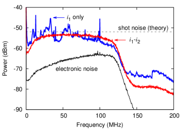
Figure 2: Noise levels measured after amplification into a bandwidth $B=1\,$kHz. Between 20 and 120 MHz, the total noise is measured from the photocurrent difference $i_{1}-i_{2}$ with a balanced optical power impinging on both photodiodes and approaches the theoretical shot noise level of -52 dBm (dashed trace) given by (1). The current $i_{1}$ of a single photodiode reveals colored classical amplitude noise. The electronic noise is measured without any optical input.

To ensure that the fluctuations at the output of the amplifier are dominated by quantum fluctuations of the vacuum field, the spectral power density at the output of the amplifier is measured (see Fig. 2). With an optical power of 3.1 mW received by each photodiode corresponding to an average photocurrent $I=1.7$ mA, a noise power of $P=-53.5\,$dBm (at 75 MHz) in a bandwidth of $B=1\,$kHz was measured. This is about 1.5 dB lower than the theoretically expected shot noise value (dashed trace) of

$$P=\frac{4eIB{R_{\rm eff}}^{2}}{Z}\approx-52\,\rm{dBm}\,,$$ (1)

where $e$ is the electron charge and $Z=50\,\Omega$ the load impedance. The difference is compatible with uncertainties in determining the transimpedance of the amplifier. The measured total noise after the amplifier has a relatively flat power density in the range of 20 to 120 MHz, while the high pass filters in the circuit suppress low frequency fluctuations. The high end of the pass band is defined by the cutoff frequency of the amplifier. To illustrate the effectiveness of removing classical noise in the photocurrents, the spectral power density of a photocurrent generated from a single diode is also shown. Strong spectral peaks at various radio frequencies appear that enter the system probably via the laser diode current. For completeness, the spectral power density of the electronic noise of the amplifier is recorded without any light input, and found to be at least 10 dB below the total noise level, i.e., the total noise is dominated by quantum fluctuations.

The amplified total noise signal is digitized into signed 16 bit wide words $x_{i}$ at a sampling rate of 60 MHz with an analog to digital converter (ADC). The sampling rate is set to be lower than the cut-off frequency of the noise signal in order to avoid temporal correlation between samples. As shown in Fig. 3, the normalized autocorrelation

$$A(d)=\langle x_{i}\,x_{i+d}\rangle_{n}/\langle x_{i}^{2}\rangle_{n}$$ (2)

evaluated over $n=10^{6}$ measured samples falls into the expected $2\sigma$ confidence interval which indicates no significant correlation between samples.

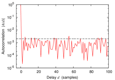
Figure 3: Autocorrelation of the total noise signal sampled at 60 MHz, computed over $10^{6}$ samples (solid line), compared with the $2\sigma$ confidence level (dashed line).

III Entropy estimation

The total noise we measured before the ADC consists of both quantum noise and the electronic noise of the detector. To determine how much randomness we can safely extract from the system in the sense that it originates from a quantum process, it is necessary to quantitatively estimate the entropy contributed by the quantum noise.

To estimate the entropy of the quantum noise $H(X_{q})$, we assume that the measured total noise signal $X_{t}=X_{q}+X_{e}$ is the sum of independent random variables $X_{q}$ for the quantum noise, and $X_{e}$ for the electronic noise.Ma et al. (2013); Sanguinetti et al. (2014). Furthermore, all three variables $X_{q}$, $X_{e}$ and $X_{t}$ are assumed to have discrete values between $-2^{15}$ and $2^{15}-1$. Since the origin of electronic noise is uncertain, we take the worst case scenario that the adversary gains full knowledge of the electronic noise, i.e., is able to predict the exact outcome of variable $X_{e}$ at any moment. In this case, the accessible amount of randomness in the acquired total noise signal is quantified by the conditional entropy $H(X_{t}|X_{e})$, i.e. the amount of entropy left in the total signal, given full knowledge of the electronic noise $X_{e}$. As the variables are assumed to be additive and independent, the conditional entropy is calculated as $H(X_{t}|X_{e})=H(X_{q}+X_{e}|X_{e})=H(X_{q}|X_{e})=H(X_{q})$.

The variance of the total noise, $\sigma_{t}^{2}$, is given by the sum of the variances $\sigma_{q}^{2}$ for the quantum noise, and $\sigma_{e}^{2}$ of the electronic noise. In an ensemble of $10^{9}$ samples, we find $\sigma_{t}=4504.41$ and $\sigma_{e}=1481.8$, which is measured by switching off the laser (see Fig. 4). Note that for the total noise, the observed distribution is slightly skewed compared to a Gaussian distribution [solid line in Fig. 4(a)]. We believe this is due to a distortion in the digitizer. Assuming the quantum noise $X_{q}$ has a Gaussian distribution Glauber (1963), we would assign $\sigma_{q}^{2}=\sigma_{t}^{2}-\sigma_{e}^{2}\approx 4253.7^{2}$. To estimate the entropy for a Gaussian distribution, we use the Shannon entropy

$$H(X_{q})=\sum_{x=-2^{15}}^{2^{15}-1}-p_{q}(x)\log_{2}p_{q}(x)\,,$$ (3)

where $p_{q}(x)$is the probability distribution of the quantum noise $X_{q}$ with variance $\sigma_{q}^{2}$. Since $\sigma_{q}\gg 1$, $H(X_{q})$ can be well approximated by

$$\int\limits_{-\infty}^{+\infty}\!\!-{f(x)}\log_{2}{f(x)}\,\mathrm{d}x=\log_{2}(\sqrt{2{\pi}e}\,\sigma_{q})\,,$$ (4)

where $f(x)$ is a Gaussian probability density function with variance $\sigma_{q}^{2}$, and $e$ the base of the natural logarithm . This yields 14.1 bits of entropy per 16-bit sample.

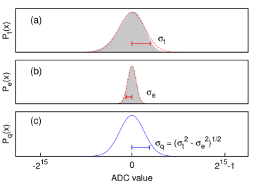
Figure 4: Probability distribution of the measured total output noise with variance ${{\sigma}_{t}}^{2}$ (a), electronic noise with variance ${{\sigma}_{e}}^{2}$ (b), and the estimated quantum noise with variance ${{\sigma}_{q}}^{2}$ (c). The filled areas in (a), (b) show the actual measurements over $10^{9}$ samples, the solid lines approximate the Gaussian distributions.

We note that this numerical estimation of entropy only serves as an upper bound of extractable randomness, i.e. the maximum possible amount of entropy one can extract from the source of randomness under the assumption of a Gaussian distribution of the independent random variables $X_{q}$ and $X_{e}$. An alternative estimation of the entropy in $X_{q}$ assumes that electronic noise is not only known to a third party, but also could be tampered withSymul, Assad, and Lam (2011); Haw et al. (2015).

IV Randomness extraction

In many applications, random numbers are required to be not only unpredictable, but also uniformly distributed. As such, the raw data at the amplifier output cannot be directly used since they are non-uniformly distributed. Randomness extraction is the essential process required to convert our biased raw data into a uniformly distributed binary stream at the final output Santha and Vazirani (1986).

Various implementations of randomness extractors have been reported, such as Trevisan’s extractor and Toeplitz-hashing extractorMa et al. (2013), random-matrix multiplicationSanguinetti et al. (2014), or the family of secure hashing algorithms (SHA)Gabriel et al. (2010).

In this work, we use a randomness extractor based on a Linear Feedback Shift Register (LFSR). The LFSRs are well known for quickly generating long pseudo-random streams with little computational resources and are in widespread use in communication applications for spectrum whiteningKrawczyk (1994); Barkan, Biham, and Keller (2007); Tkacik (2003); Wells and Ward (2004); Tsoi, Leung, and Leong (2007).

We use a maximum length LFSR with 63 memory cells and a two-element feedback path. Its state at any time step $t$ could be represented by 63 binary variables $s_{j}^{t}$, with a recursion relation

$$s_{j}^{t+1} = s_{j-1}^{t}\quad{\rm for}\,j=1\ldots 62\,,$$ (5)

$$s_{0}^{t+1} = s_{62}^{t}\oplus s_{61}^{t}\,,$$ (6)

where $\oplus$ denotes an exclusive-or operation. The 16 bit ADC word is serially injected into the feedback path (6) as $s_{0}$ with an exclusive or operation,

$$s_{0}^{t+1}=s_{62}^{t}\oplus s_{61}^{t}\oplus d^{t}\,,$$ (7)

where $d^{t}$ represents an input bit from the ADC word at time $t$. A reduced number of bits are extracted from $s_{0}$ obeying the entropy bound. To implement this efficiently in parallel for each sampled value of the vacuum field, we add a second set of memory cells, $m_{j},j=0\ldots 62$, with the recursion relations

$$m_{j}^{t+1} = s_{j}^{t}\qquad\qquad\qquad\quad\,{\rm for}\,j=0\ldots 62,$$ (8)

$$s_{j}^{t+1} = m_{j}^{t}\oplus m_{j+1}^{t}\oplus d_{j}^{t}\quad{\rm for}\,j=0\ldots 61,$$ (9)

$$s_{62}^{t+1} = m_{62}^{t}\oplus s_{0}^{t}$$ (10)

where $d_{j}^{t}$ represents the $j$-th bit of the ADC word sampled at $t$ for $j<16$, and $d_{j}^{t}=0$ for $j\geq 16$. Recursion relations (8-10) are equivalent to the operation described in (7), but with all input bits $d_{j}^{t}$ of one sampled word injected at once instead of serially. The output bit stream is a snapshot of eight cells $m_{j}$ with $j=0,2,4...14$, extracted at the ADC sampling rate (60 MHz). The extraction ratio of 50% is lower than $14.1/16\approx 88\%$ from the entropy bound estimated in (4). The recursion equations (8-10) and the reduced rate extraction is implemented in a complex programmable logical device (CPLD, Model LC4256 from Lattice semiconductor).

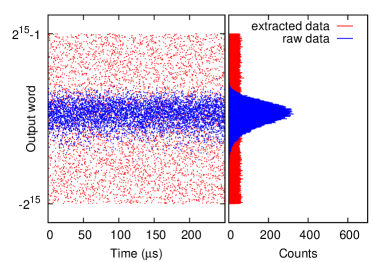
Figure 5: Distribution of random data before (blue) and after (red) the randomness extractor, shown in time domain (left) and histogram (right).

A merit of this extractor is its low circuit complexity. Unlike many secure hashing algorithms, it can be easily implemented either in high speed or low power technology. Therefore, the extraction process does not limit the random number generation rate. This scheme can receive a parallel injection of up to 63 raw bits per clock cycle while still following the extractor equations (5) and (7). With the CPLD operating at its maximum clock frequency (400 MHz), this algorithm would be able to process up to $25\times 10^{9}$ raw input bits per second.

V Performance

To evaluate the quality of the extracted random numbers, we apply two suites of randomness tests: the statistical test suite from NIST Rukhin et al. (2010), and the “Die-harder” randomness test battery Robert G. Brown (2004). The output of our RNG passed both tests consistently when evaluated over a sample of 400 Gigabit.

Our implementation reaches an output rate of 480 Mbit/s of uniformly distributed random bits, with the digitizer unit sampling at 60 MHz and randomness extraction ratio of 50%; this is limited by the speed limit of the data transmission protocol we use (USB2.0). With a different transmission protocol but the same ADC sampling, we could extract a random bit rate of up to 60 MHz$\times 14.1$ bits or 846 Mbit/s. With moderate effort, the random number generation rate can be greatly increased by extending the bandwidth of the photodiodes, amplifiers, and digitizer devices, while maintaining the relatively simple randomness extraction mechanism. Practically, the resolution-bandwidth product of the ADC will then limit the random bit generation rate.

VI Conclusion

In summary, we demonstrated a random number generation scheme by measuring the vacuum fluctuations of the electromagnetic field. By estimating the amount of usable entropy from quantum noise and using an efficient randomness extractor based on linear feedback shift registers, we are able to generate uniformly distributed random numbers at a high rate from a fundamentally unpredictable quantum measurement.

We acknowledge the support of this work by the National Research Foundation (partly under grant No. NRF-CRP12-2013-03) & Ministry of Education in Singapore, partly through the Academic Research Fund MOE2012-T3-1-009.

References

- Gisin et al. (2002) N. Gisin, G. Ribordy, W. Tittel, and H. Zbinden, Rev. Mod. Phys. 74, 145–195 (2002).
- Metropolis (1987) N. Metropolis, Los Alamos Science 15, 125 (1987).
- Galton (1890) F. Galton, Nature 42, 13–14 (1890).
- Jun and Kocher (1999) B. Jun and P. Kocher, “The intel random number generator,” Tech. Rep. (Cryptography Research Inc., 1999).
- Gude (1985) M. Gude, Frequenz 39, 187 (1985).
- Figotin et al. (2004) A. Figotin, I. Vitebskiy, V. Popovich, G. Stetsenko, S. Molchanov, A. Gordon, J. Quinn, and N. Stavrakas, “Random number generator based on the spontaneous alpha-decay,” (2004), uS Patent 6,745,217.
- Stipcevic and Rogina (2007) M. Stipcevic and B. M. Rogina, Rev. Sci. Instrum. 78, 045104 (2007).
- Wayne et al. (2009) M. A. Wayne, E. R. Jeffrey, G. M. Akselrod, and P. G. Kwiat, Journal of Modern Optics 56, 516 (2009).
- Fürst et al. (2010) M. Fürst, H. Weier, S. Nauerth, D. G. Marangon, C. Kurtsiefer, and H. Weinfurter, Optics Express 18, 13029 (2010).
- Wayne and Kwiat (2010) M. A. Wayne and P. G. Kwiat, Opt. Express 18, 9351 (2010).
- Wahl et al. (2011) M. Wahl, M. Leifgen, M. Berlin, T. Röhlicke, H.-J. Rahn, and O. Benson, Applied Physics Letters 98, 171105 (2011).
- Jennewein et al. (2000) T. Jennewein, U. Achleitner, G. Weihs, H. Weinfurter, and A. Zeilinger, Review of Scientific Instruments 71, 1675 (2000).
- Stefanov et al. (2000) A. Stefanov, N. Gisin, O. Guinnard, L. Guinnard, and H. Zbinden, Journal of Modern Optics 47, 595 (2000).
- Frauchiger and Renner (2013) D. Frauchiger and R. Renner, Emerging Technologies in Security and Defence; and Quantum Security II; and Unmanned Sensor Systems X (2013), 10.1117/12.2032183.
- Williams et al. (2010) C. R. S. Williams, J. C. Salevan, X. Li, R. Roy, and T. E. Murphy, Optics Express 18, 23584 (2010).
- Gabriel et al. (2010) C. Gabriel, C. Wittmann, D. Sych, R. Dong, W. Mauerer, U. L. Andersen, C. Marquardt, and G. Leuchs, Nature Photon 4, 711–715 (2010).
- Symul, Assad, and Lam (2011) T. Symul, S. M. Assad, and P. K. Lam, Applied Physics Letters 98, 231103 (2011).
- Shen, Tian, and Zou (2010) Y. Shen, L. Tian, and H. Zou, Physical Review A 81 (2010), 10.1103/physreva.81.063814.
- Kanter et al. (2009) I. Kanter, Y. Aviad, I. Reidler, E. Cohen, and M. Rosenbluh, Nature Photon 4, 58–61 (2009).
- Sanguinetti et al. (2014) B. Sanguinetti, A. Martin, H. Zbinden, and N. Gisin, Phys. Rev. X 4, 031056 (2014), 1405.0435 .
- Qi et al. (2010) B. Qi, Y.-M. Chi, H.-K. Lo, and L. Qian, Opt. Lett. 35, 312 (2010).
- Xu et al. (2012) F. Xu, B. Qi, X. Ma, H. Xu, H. Zheng, and H.-K. Lo, Optics Express 20, 12366 (2012).
- Abellán et al. (2014) C. Abellán, W. Amaya, M. Jofre, M. Curty, A. Acín, J. Capmany, V. Pruneri, and M. W. Mitchell, Optics Express 22, 1645 (2014).
- Abellán et al. (2015) C. Abellán, W. Amaya, D. Mitrani, V. Pruneri, and M. W. Mitchell, Phys. Rev. Lett. 115, 250403 (2015).
- Yuan et al. (2014) Z. L. Yuan, M. Lucamarini, J. F. Dynes, B. Fröhlich, A. Plews, and A. J. Shields, Applied Physics Letters 104, 261112 (2014).
- Jakeman, Oliver, and Pike (1975) E. Jakeman, C. Oliver, and E. Pike, Advances in Physics 24, 349 (1975).
- Yuen and Chan (1983) H. P. Yuen and V. W. Chan, Optics Letters 8, 177 (1983).
- Glauber (1963) R. J. Glauber, Phys. Rev. 131, 2766 (1963).
- Schumaker (1984) B. L. Schumaker, Optics Lettes 9, 189 (1984).
- Ma et al. (2013) X. Ma, F. Xu, H. Xu, X. Tan, B. Qi, and H.-K. Lo, Phys. Rev. A 87, 062327 (2013).
- Note (1) One can show that bit for .
- Haw et al. (2015) J. Y. Haw, S. M. Assad, A. M. Lance, N. H. Y. Ng, V. Sharma, P. K. Lam, and T. Symul, Phys. Rev. Applied 3, 054004 (2015).
- Santha and Vazirani (1986) M. Santha and U. V. Vazirani, J. Comput. Syst. Sci. 33, 75 (1986).
- Krawczyk (1994) H. Krawczyk, Advances in Cryptology — CRYPTO ’94 , 129–139 (1994).
- Barkan, Biham, and Keller (2007) E. Barkan, E. Biham, and N. Keller, J Cryptol 21, 392–429 (2007).
- Tkacik (2003) T. E. Tkacik, in Cryptographic Hardware and Embedded Systems - CHES 2002, Lecture Notes in Computer Science, Vol. 2523, edited by B. S. Kaliski, c. K. Koç, and C. Paar (Springer Berlin Heidelberg, 2003) pp. 450–453.
- Wells and Ward (2004) S. Wells and D. Ward, “Random number generator with entropy accumulation,” (2004), uS Patent 6,687,721.
- Tsoi, Leung, and Leong (2007) K. Tsoi, K. Leung, and P. Leong, Computers Digital Techniques, IET 1, 349 (2007).
- Rukhin et al. (2010) A. Rukhin, J. Soto, J. Nechvatal, M. Smid, E. Barker, S. Leigh, M. Levenson, M. Vangel, D. Banks, A. Heckert, J. Dray, and S. Vo, A Statistical Test Suite for Random and Pseudorandom Number Generators for Cryptographic Applications, National Institute of Standards and Technology (2010).
- Robert G. Brown (2004) D. B. Robert G. Brown, Dirk Eddelbuettel, “Dieharder: A random number test suite,” (2004).