Relativistic quantum-statistical distributions

Generation of random deviates for relativistic quantum-statistical distributions

Abstract

We provide an algorithm for generation of momenta (or energies) of relativistic particles according to the relativistic Bose-Einstein or Fermi-Dirac distributions. The algorithm uses rejection method with effectively selected comparison function so that the acceptance rate of the generated values is always better than 0.9. It might find its use in Monte-Carlo generators of particles from reactions in high-energy physics.

52W20

1 Motivation

In projects related to multiparticle production in hadronic or nuclear collisions it is often demanded to generate a large number of particles with momenta distributed according to relativistic Bose-Einstein of Fermi-Dirac distribution. Here one has to take into account the total energy (i.e. including the mass) when evaluating the exponent of the distributions

$$f(\vec{p})=\frac{1}{(2\pi\hbar)^{3}}\left[\exp\left(\frac{c\sqrt{m^{2}c^{2}+p^{2}}-\mu}{k_{B}T}\right)+q\right]^{-1}$$ (1)

where $m$ is the mass of the particles, $p=|\vec{p}|$, $\mu$ is the chemical potential and $T$ is temperature. Parameter $q$ assumes the value of 1 for fermions and $-1$ for bosons. For the generation of invariant momentum distributions one also needs this distribution multiplied with the energy

$$S(\vec{p})=\frac{c\sqrt{m^{2}c^{2}+p^{2}}}{(2\pi\hbar)^{3}}\left[\exp\left(\frac{c\sqrt{m^{2}c^{2}+p^{2}}-\mu}{k_{B}T}\right)+q\right]^{-1}$$ (2)

As the distribution is spherically symmetric, the angles are trivially integrated and we are left with the distributions for the size of the momentum vector. In order to make it suitable for a general procedure, it is expressed with the help of dimensionless variable

$$x=\frac{p}{mc}\,.$$ (3)

Thus we get

$$f(x)=x^{2}\,\left[\exp\left(A(\sqrt{1+x^{2}}-M)\right)+q\right]^{-1}$$ (4)

or for the other distribution

$$S(x)=\sqrt{1+x^{2}}\,x^{2}\,\left[\exp\left(A(\sqrt{1+x^{2}}-M)\right)+q\right]^{-1}\,,$$ (5)

where

$$A=\frac{mc^{2}}{k_{B}T}\,,\qquad M=\frac{\mu}{mc^{2}}\,.$$ (6)

In these functions we have suppressed the constant pre-factors which also contain dimensions.

For the Monte Carlo generation we shall proceed with the dimensionless distributions without the dimensionfull pre-factors.

A similar algorithm for the generation of relativistic Maxwellian distribution has been reported in [1, 2]. In our work we properly account for quantum statistics and allow for non-zero chemical potential, which can influence the momentum distribution. We describe the procedure for the distribution (5) with the energy factor. The procedure for the distribution (4) can easily be derived along the same steps as we shall proceed.

2 The algorithm

We demonstrate in the Apendix that the distribution (5) is log-concave for large enough $x$, i.e. its logarithm is a concave function. For such a distribution there always exists an exponential that is everywhere above the demanded distribution. One can generate random deviates according to the exponential and use the rejection method[2].

In order to achieve smallest possible rejection rate we use piecewise analytic comparison function, as indicated in Fig. 1.

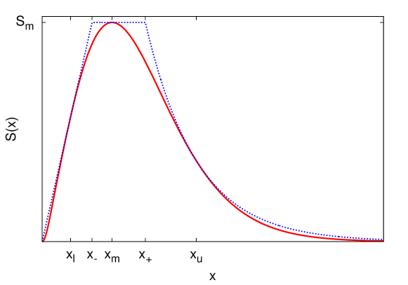
Figure 1: Dimensionless Bose-Einstein distribution with energy pre-factor according to Eq. (5). The shape corresponds to $A=2/3$ and $M=3/4$ but we have suppressed the values on the axes in order to demonstrate the comparison function and locate the important points for the determination of the comparison function.

The three pieces are determined so that

• for $x\leq x_{-}$ the comparison function is linear;

• for $x_{-}<x\leq x_{+}$ the comparison function is constant and equal to the value of the distribution at the mode;

• for $x>x_{+}$ the comparison function is exponential.

The joint points $x_{-}$ and $x_{+}$ are chosen so that the comparison function is always continuous.

For the determination of the comparison function we thus need to determine the five points indicated on the horizontal axis.

$x_{m}$ The mode of $S(x)$. This is obtained easily by differentiating and we get

$$2+3x_{m}^{2}-\frac{Ax_{m}^{2}\sqrt{1+x_{m}^{2}}}{1+q\exp\left(-A(\sqrt{1+x_{m}^{2}}-M)\right)}=0\,.$$ (7)

Unfortunately this expression cannot be solved analytically and numerical methods must be invoked.

Subsequently, the value of $S(x)$ at the mode can be determined

$$S_{m}=S(x_{m})=\sqrt{1+x_{m}^{2}}\,x_{m}^{2}\,\left[\exp\left(A(\sqrt{1+x_{m}^{2}}-M)\right)+q\right]^{-1}\,.$$ (8)

$x_{l}$ The point left from the mode in which the linear comparison function touches the distribution. It is found from the condition for the derivative of the distribution

$$\left.\frac{dS(x)}{dx}\right|_{x=x_{l}}=\frac{S(x_{l})}{x_{l}}$$

which leads to

$$1+2x_{l}^{2}-\frac{Ax_{l}^{2}\sqrt{1+x_{l}^{2}}}{1+q\exp\left(-A(\sqrt{1+x_{l}^{2}}-M)\right)}=0\,.$$ (9)

The slope of the liner comparison function is then

$$K=\frac{S(x_{l})}{x_{l}}=\frac{x_{l}\sqrt{1+x_{l}^{2}}}{\exp\left(A(\sqrt{1+x_{l}^{2}}-M)\right)+q}\,.$$ (10)

$x_{-}$ The point in which the linear part of the comparison function and its constant part meet. It can be determined as

$$x_{-}=\frac{S_{m}}{x_{l}\sqrt{1+x_{l}^{2}}}\left[\exp\left(A(\sqrt{1+x_{l}^{2}}-M)\right)+q\right]\,.$$ (11)

The knowledge of $x_{-}$ also allows to express

$$K=\frac{S_{m}}{x_{-}}\,.$$ (12)

$x_{u}$ The point in which the exponential part of the comparison function touches the distribution. Above the mode the distribution is log-concave. Therefore, $x_{u}$ can be chosen anywhere above $x_{m}$. However, we checked that, the acceptance rate is optimised with $x_{u}$ chosen so that the distribution there drops to $1/e$ of its maximum value. We get the value by solving the equation for the logarithms of the distribution

$$\ln S(x_{u})=\ln S_{m}-1\,,$$

which leads to

$$1-\ln S_{m}+\frac{1}{2}\ln(1+x_{u}^{2})+2\ln x_{u}-\ln\left[\exp\left(A(\sqrt{1+x_{u}^{2}}-M)\right)+q\right]=0\,.$$ (13)

Again, this equation must be solved numerically.

Once $x_{u}$ is determined, we can determine the slope parameter of the exponential comparison function. It is given by the logarithm of the distribution. Thus

$$\lambda=-\left.\frac{d\ln S(x)}{dx}\right|_{x=x_{u}}=\frac{x_{u}}{\sqrt{1+x_{u}^{2}}}\left[1-A\frac{\exp\left(A(\sqrt{1+x_{u}^{2}}-M)\right)}{\exp\left(A(\sqrt{1+x_{u}^{2}}-M)\right)+q}\right]-\frac{2}{x_{u}}\,.$$ (14)

$x_{+}$ Finally, this is the point in which the constant part of the comparison function and its exponential part join. It is determined from a simple equation

$$x_{+}=x_{u}-\frac{1}{\lambda}\,.$$ (15)

Once we have $x_{+}$, we also know the exponential part of the comparison function which reads

$$S^{\prime}(x)=S_{m}e^{-\lambda(x-x_{+})}\,.$$ (16)

Thus we can formulate the comparison function

$$S^{\prime}(x)=\left\{\begin{array}[]{lcl}\frac{S_{m}}{x_{-}}x&:&x\leq x_{-}\\ S_{m}&:&x_{-}<x\leq x_{+}\\ S_{m}e^{-\lambda(x-x_{+})}&:&x>x_{+}\end{array}\right.$$ (17)

In order to use this comparison function as probability density (after normalisation) for random variate generation we need the values

$$y_{-} = \int_{0}^{x_{-}}S^{\prime}(x)dx=\frac{1}{2}S_{m}x_{-}$$ (18a)

$$y_{+} = \int_{0}^{x_{+}}S^{\prime}(x)dx=S_{m}\left(x_{+}-\frac{1}{2}x_{-}\right)$$ (18b)

$$y_{\infty} = \int_{0}^{\infty}S^{\prime}(x)dx=S_{m}\left(x_{+}-\frac{1}{2}x_{-}+\frac{1}{\lambda}\right)\,.$$ (18c)

The inverse if the integral of $S^{\prime}(x)$ is

$$x(y)=\left\{\begin{array}[]{lclcl}\sqrt{\frac{2x_{-}y}{S_{m}}}&:&y\leq y_{-}&\mathrm{gives}&x\leq x_{-}\\ \frac{1}{2}x_{-}+\frac{y}{S_{m}}&:&y_{-}<y\leq y_{+}&\mathrm{gives}&x_{-}<x\leq x_{+}\\ x_{+}-\frac{1}{\lambda}\ln\left[1+\left(x_{+}-\frac{1}{2}x_{-}\right)\lambda-\frac{\lambda}{S_{m}}y\right]&:&y_{+}<y\leq y_{\infty}&\mathrm{gives}&x>x_{+}\end{array}\right.$$ (19)

For the rejection step we need the probabilities to accept the generated value of $x$. They are given as ${\cal P}(x)=S(x)/S^{\prime}(x)$. In the three intervals they read

$${\cal P}(x) =\frac{x_{-}x\sqrt{1+x^{2}}}{S_{m}\left[\exp\left(A(\sqrt{1+x^{2}}-M)\right)+q\right]} : x\leq x_{-}$$ (20a)

$${\cal P}(x) =\frac{x^{2}\sqrt{1+x^{2}}}{S_{m}\left[\exp\left(A(\sqrt{1+x^{2}}-M)\right)+q\right]} : x_{-}<x\leq x_{+}$$ (20b)

$${\cal P}(x) =\frac{x^{2}\sqrt{1+x^{2}}\exp\left(\lambda(x-x_{+})\right)}{S_{m}\left[\exp\left(A(\sqrt{1+x^{2}}-M)\right)+q\right]} : x_{+}<x$$ (20c)

Now we have collected all expressions needed to build up the algorithm. Because of the need to numerically solve a few equations the procedure may be lengthy if one needs to generate just one random value. However, if many values must be generated for the same temperature, chemical potential and particle mass, then all parameters can be calculated first and then used repeatedly. Thus the first part of the algorithm is the calculation of the parameters:

1. Determine $x_{m}$ by solving Eq. (7).

2. Calculate $S_{m}$ from Eq. (8).

3. Determine $x_{l}$ by solving Eq. (9).

4. Calculate $x_{-}$ from Eq. (11).

5. Determine $x_{u}$ by solving Eq (13).

6. Calculate $\lambda$ from Eq. (14).

7. Calculate $x_{+}$ from Eq. (15).

8. For later convenience calculate also the values of $y_{-}$, $y_{+}$, and $y_{\infty}$ from Eqs. (18).

This is the common part of the preparation. Then, in order to generate a value, follow these steps:

1. Generate uniform random deviate $y$ from the interval $[0,y_{\infty}]$.

2. Calculate $x=x(y)$ from Eq. (19).

3. Accept the value of $x$ with the probability given by Eqs. (20). If the value is not accepted, return to step 9.

3 Illustration of results

We have tested this algorithm in wide range of parameters $A$ and $M$. Particle masses were chosen both smaller than temperature so that large momenta are available and also much larger than temperature so that the momenta are practically non-relativistic. Chemical potentials up to the value of particle mass for bosons, i.e. the point of condensation, were tested, as well (Figure 2). In all cases the acceptance rate was around 90%. This shows that the comparison function is very well adapted to the present problem.

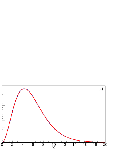
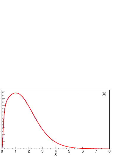
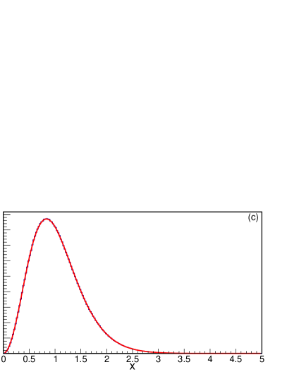
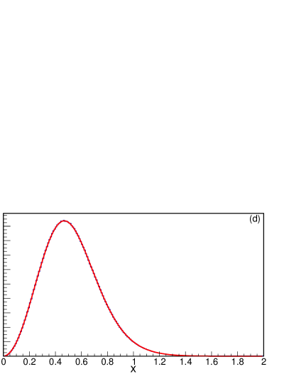
Figure 2: Histograms of $10^{7}$ random deviates fitted by function $S(x)$ with only the absolute normalisation as a fit parameter. Values of $A$ and $M$ are fixed in the fit function in order to be the same as in the Monte Carlo generation. The values are: (a) $A=2/3$, $M=0$, bosons (e.g. pions with $\mu=0$ at temperature $k_{B}T=207$ MeV); (b) $A=2$, $M=0.993$, bosons (e.g. pions with $\mu=137$ MeV$/c^{2}$ at temperature $k_{B}T=69$ MeV, close to condensation); (c) $A=4.536$, $M=0$, fermions (e.g. protons with $\mu=0$ at temperature $k_{B}T=(3/2)m_{\pi}c^{2}=207$ MeV); (d) $A=13.609$, $M=0.9989$, fermions (e.g. protons with $\mu=938$ MeV at temperature $k_{B}T=m_{\pi}c^{2}/2=69$ MeV).

4 Conclusions

The presented algorithm has been successfully implemented in an upgrade of the Monte Carlo event generator DRAGON [3], which serves for the generation of hadrons produced in high energy nuclear collisions. It is, however, general and can serve in any other application where relativistic momenta must be generated from quantum-statistical distributions.

Appendix A Log-concave distribution

In this Appendix we demonstrate that the distribution $S(x)$ according to Eq. (5) is indeed log-concave on the interval above the mode. Therefore, an exponential function which touches $S(x)$ from above in one point will never be smaller than $S(x)$.

The calculation is straightforward. We take the second derivative of $\ln S(x)$. For fermions $(q=1)$, this leads to

$$\frac{d^{2}\ln S(x)}{dx^{2}}=-\frac{1}{1+x^{2}}\left\{\frac{2}{x^{2}}+1+\frac{2x^{2}}{1+x^{2}}+\frac{A}{\sqrt{1+x^{2}}}\left(1-s_{f}(x)\right)+A^{2}x^{2}s_{f}(x)\left(1-s_{f}(x)\right)\right\}$$ (21)

where

$$s_{f}(x)=\frac{1}{\exp\left[A(\sqrt{1+x^{2}}-M)\right]+1}\,.$$

Note that $s_{f}(x)\leq 1$ for any $x$. Therefore, $(1-s_{f}(x))\geq 0$ and all terms in the bracket in Eq. (21) are non-negative. In summary, we see that for fermions

$$\frac{d^{2}\ln S(x)}{dx^{2}}<0$$ (22)

and thus the distribution is log-concave everywhere.

The case of bosons is slightly more involved. Again, we take the second derivative

$$\frac{d^{2}\ln S(x)}{dx^{2}}=-\frac{1}{1+x^{2}}\left\{\frac{2}{x^{2}}+1+\frac{2x^{2}}{1+x^{2}}+\frac{A}{\sqrt{1+x^{2}}}\left(1+s_{b}(x)\right)-A^{2}x^{2}s_{b}(x)\left(1+s_{b}(x)\right)\right\}$$ (23)

where

$$s_{b}(x)=\frac{1}{\exp\left[A(\sqrt{1+x^{2}}-M)\right]-1}\,.$$

Note the change of the sign in $(1+s_{b}(x))$ and in front of the last term. Due to this, for bosons the second derivative may become positive in some cases. We want to demonstrate that such pathological intervals are always below the mode of $S(x)$.

For $x\to\infty$ the terms $s_{b}(x)$ go to 0 exponentially (we chose the letter $s$ for “small”), and one can inspect that

$$\lim_{x\to\infty}\frac{d^{2}\ln S(x)}{dx^{2}}=0\,$$

and the value of the limit is being approached from below. Thus the second derivative is either negative everywhere or there is a point $x=x_{c}$ where it crosses the horizontal axis and stays negative for $x>x_{c}$. It is enough to show that $x_{c}<x_{m}$.

It turns out that the second derivative becomes positive only if the particles are light with $A\leq 3$ and $M$ is close to 1, which is quite an extreme case. (Recall that for bosons $M$ must be smaller than 1 and $M=1$ corresponds to the condensation point where the distribution does no longer apply.) In such a case, for small values of $x$ one obtains $s_{b}\gg 1$ and the last term in Eq. (23) prevails. We have scanned the whole relevant parameter region of $A$ and $M$ and checked that always $x_{c}<x_{m}$ (Figure 3).

Figure 3: The difference in positions $x_{m}-x_{c}$ as function of $A$ and $M$. Values are not plotted if the second derivative $d^{2}\ln S(x)/dx^{2}$ for bosons stays negative everywhere. One sees that always $x_{c}<x_{m}$.

In all other cases the function $S(x)$ is log-concave everywhere.

We conclude that it is safe to use the exponential comparison function in the interval $(x_{m},\infty)$.