Robust Sound Source Localization Using a Microphone Array on a Mobile Robot

Abstract

The hearing sense on a mobile robot is important because it is omnidirectional and it does not require direct line-of-sight with the sound source. Such capabilities can nicely complement vision to help localize a person or an interesting event in the environment. To do so the robot auditory system must be able to work in noisy, unknown and diverse environmental conditions. In this paper we present a robust sound source localization method in three-dimensional space using an array of 8 microphones. The method is based on time delay of arrival estimation. Results show that a mobile robot can localize in real time different types of sound sources over a range of 3 meters and with a precision of $3^{\circ}$.

1 Introduction

Compared to vision, robot audition is in its infancy: while research activities on automatic speech recognition are very active, the use and the adaptation of these techniques to the context of mobile robotics has only been addressed by a few. There is the SAIL robot that uses one microphone to develop online audio-driven behaviors [7]. The robot ROBITA [2] uses 2 microphones to follow a conversation between two persons. The humanoid robot SIG [4, 5] uses two pairs of microphones, one pair installed at the ear position of the head to collect sound from the external world, and the other placed inside the head to collect internal sounds (caused by motors) for noise cancellation. Like humans, these last two robots use binaural localization, i.e., the ability to locate the source of sound in three dimensional space.

However, it is a difficult challenge to only use a pair of microphones on a robot to match the hearing capabilities of humans. The human hearing sense takes into account the acoustic shadow created by the head and the reflections of the sound by the two ridges running along the edges of the outer ears. With a pair of microphones, only localization in two dimensions is possible, without being able to distinguish if the sounds come from the front or the back of the robot. Also, it may be difficult to get high precision readings when the sound source is in the same axis of the pair of microphones.

It is not necessary to limit robots to a human-like auditory system using only two microphones. Our strategy is to use more microphones to compensate for the high level of complexity in the human auditory system. This way, increased resolution can be obtained in three-dimensional space. This also means increased robustness, since multiple signals allow to filter out noise (instead of trying to isolate the noise source by putting sensors inside the robot’s head, as with SIG) and discriminate multiple sound sources. It is with these potential benefits in mind that we developed a sound source localization method based on time delay of arrival (TDOA) estimation using an array of 8 microphones. The method works for far-field and near-field sound sources and is validated using a Pioneer 2 mobile robotic platform.

The paper is organized as follows. Section 2 presents the principles behing TDOA estimation. Section 3 explains how the position of the sound source is derived from the TDOA, followed by experimental results in Section 4.

2 TDOA Estimation

We consider windowed frames of $N$ samples with 50% overlap. For the sake of simplicity, the index corresponding to the frame is ommitted from the equations. In order to determine the delay in the signal captured by two different microphones, it is necessary to define a coherence measure. The most common coherence measure is a simple cross-correlation between the signals perceived by two microphones, as expressed by:

$$R_{ij}(\tau)=\sum_{n=0}^{N-1}x_{i}[n]x_{j}[n-\tau]$$ (1)

where $x_{i}[n]$ is the signal received by microphone $i$ and $\tau$ is the correlation lag in samples. The cross-correlation $R_{ij}(\tau)$ is maximal when $\tau$ is equal to the offset between the two received signals. The problem with computing the cross-correlation using Equation 1 is that the complexity is $\mathcal{O}\left(N^{2}\right)$. However, it is possible to compute an approximation in the frequency domain by computing the inverse Fourier transform of the cross-spectrum, reducing the complexity to $\mathcal{O}\left(N\log_{2}N\right)$. The correlation approximation is given by:

$$R_{ij}(\tau)\approx\sum_{k=0}^{N-1}X_{i}(k)X_{j}(k)^{*}e^{\imath 2\pi k\tau/N}$$ (2)

where $X_{i}(k)$ is the discrete Fourier transform of $x_{i}[n]$ and $X_{i}(k)X_{j}(k)^{*}$ is the cross-spectrum of $x_{i}[n]$ and $x_{j}[n]$.

A major limitation of that approach is that the correlation is strongly dependent on the statistical properties of the source signal. Since most signals, including voice, are generally low-pass, the correlation between adjacent samples is high and generates cross-correlation peaks that can be very wide.

The problem of wide cross-correlation peaks can be solved by whitening the spectrum of the signals prior to computing the cross-correlation [6]. The resulting “whitened cross-correlation” is defined as:

$$R_{ij}^{(w)}(\tau)=\sum_{k=0}^{N-1}\frac{X_{i}(k)X_{j}(k)^{*}}{\left|X_{i}(k)\right|\left|X_{j}(k)\right|}e^{\imath 2\pi k\tau/N}$$ (3)

and corresponds to the inverse Fourier transform of the normalized (whitened) cross spectrum.

Whitening allows to only take the phase of $X_{i}(k)$ into account, giving each frequency component the same weight and narrowing the wide maxima caused by correlations within the received signal. Figure 1 shows the spectrogram of the noisy signal as received by one of the microphones in the array. The corresponding whitened cross-correlation in Figure 2 shows peaks at the same time as the sources found in Figure 1.

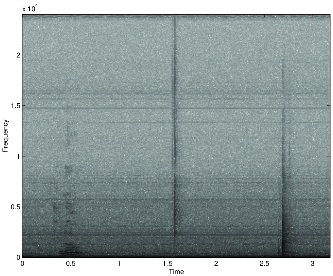
Figure 1: Spectrogram of the signal received at microphone 1 ($X_{1}(k)$) for the following sounds: speech at 0.5 sec, finger snap at 1.5 sec and boot noise on the floor at 2.7 sec.

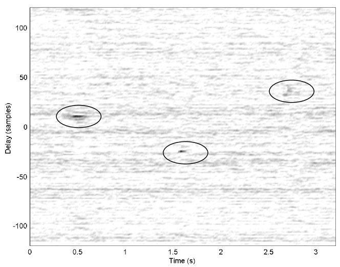
Figure 2: Whitened cross-correlation $R_{ij}^{(w)}(\tau)$ with peaks (circled) corresponding to the sound sources.

2.1 Spectral Weighting

The whitened cross-correlation method explained in the previous subsection has several drawbacks. Each frequency bin of the spectrum contributes the same amount to the final correlation, even if the signal at that frequency is dominated by noise. This makes the system less robust to noise, while making detection of voice (which has a narrow bandwidth) more difficult.

In order to counter the problem, we developed a new weighting function of the spectrum. This gives more weight to regions in the spectrum where the local signal-to-noise ratio (SNR) is the highest. Let $X(k)$ be the mean power spectral density for all the microphones at a given time and $X_{n}(k)$ be a noise estimate based on the time average of previous $X(k)$. We define a noise masking weight by:

$$w(k)=\max\left(0.1,\frac{X(k)-\alpha X_{n}(k)}{X(k)}\right)$$ (4)

where $\alpha<1$ is a coefficient that makes the noise estimate more conservative. $w(k)$ becomes close to 0 in regions that are dominated by noise, while $w(k)$ is close to 1 in regions where the signal is much stronger than the noise. The second part of the weighting function is designed to increase the contribution of tonal regions of the spectrum (where the local SNR is very high). Starting from Equation 4, we define the enhanced weighting function $w_{e}(k)$ as:

$$w_{e}(k)=\left\{\begin{array}[]{ll}w(k)&,\>X(k)\leq X_{n}(k)\\ w(k)\left(\frac{X(k)}{X_{n}(k)}\right)^{\gamma}&,\>X(k)>X_{n}(k)\end{array}\right.$$ (5)

where the exponent $0<\gamma<1$ gives more weight to regions where the signal is much higher than the noise. For our system, we empirically set $\alpha$ to 0.4 and $\gamma$ to 0.3. The resulting weighted cross-correlation is defined as:

$$R_{ij}^{(e)}(\tau)=\sum_{k=0}^{N-1}\frac{w_{e}^{2}(k)X_{i}(k)X_{j}(k)^{*}}{\left|X_{i}(k)\right|\left|X_{j}(k)\right|}e^{\imath 2\pi k\tau/N}$$ (6)

The value of $w_{e}(k)$ as a function of time is shown in Figure 3 and the resulting cross-correlation is shown in Figure 4. Compared to Figure 2 it is possible to see that the cross-correlation has less noise, although the peaks are slightly wider. Nonetheless, the weighting method increases the robustness of TDOA estimation.

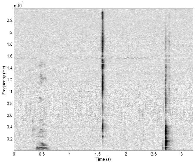
Figure 3: Noise weighting $w_{e}(k)$ for the sound sources

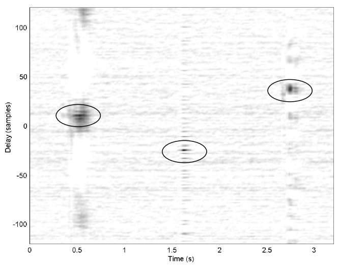
Figure 4: Cross-correlation with noise-weighting $R_{ij}^{(e)}(\tau)$ with peaks (circled) corresponding to the sound sources.

2.2 TDOA Estimation Using $N$ Microphones

The time delay of arrival (TDOA) between microphones $i$ and $j$; $\Delta T_{ij}$ can be found by locating the peak in the cross-correlation as:

$$\begin{array}[]{ccc}\Delta T_{ij}=&\mathrm{argmax}&R_{ij}^{(e)}(\tau)\\ &\tau\end{array}$$ (7)

Using an array of $N$ microphones, it is possible to compute $N(N-1)/2$ different cross-correlations of which only $N-1$ are independent. We chose to work only with the $\Delta T_{1i}$ values ($\Delta T_{12}$ to $\Delta T_{18}$), the remaining ones being derived by:

$$\Delta T_{ij}=\Delta T_{1j}-\Delta T_{1i}$$ (8)

The number of false detections can be reduced by considering sources to be valid only when Equation 8 is satisfied for all $i\neq j$.

Since in practice the highest peak may be caused by noise, we extract the $M$ highest peaks in each cross-correlation (where $M$ is set empirically to 8) and assume that one of them represents the real value of $\Delta T_{ij}$. This leads to a search through all possible combinations of $\Delta T_{1i}$ values (there are a total of $M^{N-1}$ combinations) that satisfy Equation 8 for all dependent $\Delta T_{ij}$. For example, in the case of an array of 8 microphones, there are 7 independent delays ($\Delta T_{12}$ to $\Delta T_{18}$), but a total of 21 constraints (e.g. $\Delta T_{23}=\Delta T_{13}-\Delta T_{12}$), which makes it very unlikely to falsely detect a source. When more than one set of $\Delta T_{1i}$ values respect all the constraints, only the one with the greatest correlation values is retained and used to find the direction of the source using the method presented in Section 3.

3 Position Estimation

Once TDOA estimation is performed, it is possible to compute the position of the source through geometrical calculations. One technique based on a linear equation system [1] but sometimes, depending on the signals, the system is ill-conditioned and unstable. For that reason, a simpler model based on far field assumption is used.

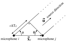
Figure 5: Computing source direction from TDOA.

Figure 5 illustrates the case of a 2 microphone array with a source in the far-field. Using the cosine law, we can state that:

$$\cos\phi=\frac{\vec{\mathbf{u}}\cdot\vec{\mathbf{x}}_{ij}}{\left\|\vec{\mathbf{u}}\right\|\left\|\vec{\mathbf{x}}_{ij}\right\|}=\frac{\vec{\mathbf{u}}\cdot\vec{\mathbf{x}}_{ij}}{\left\|\vec{\mathbf{x}}_{ij}\right\|}$$ (9)

where $\vec{\mathbf{x}}_{ij}$ is the vector that goes from microphone $i$ to microphone $j$ and $\vec{\mathbf{u}}$ is a unit vector pointing in the direction of the source. From the same figure, it can be stated that:

$$\cos\phi=\sin\theta=\frac{c\Delta T_{ij}}{\left\|\vec{\mathbf{x}}_{ij}\right\|}$$ (10)

where $c$ is the speed of sound. When combining equations 9 and 10, we obtain:

$$\vec{\mathbf{u}}\cdot\vec{\mathbf{x}}_{ij}=c\Delta T_{ij}$$ (11)

which can be re-written as:

$$u\left(x_{j}-x_{i}\right)+v\left(y_{j}-y_{i}\right)+w\left(z_{j}-z_{i}\right)=c\Delta T_{ij}$$ (12)

where $\vec{\mathbf{u}}=(u,\>v,\>w)$ and $\vec{\mathbf{x}}_{ij}=\left(x_{j}-x_{i},\>y_{j}-y_{i},\>z_{j}-z_{i}\right)$, the position of microphone $i$ being $\left(x_{i},\>y_{i},\>z_{i}\right)$. Considering $N$ microphones, we obtain a system of $N-1$ equations:

$$\begin{array}[]{c}\left[\begin{array}[]{ccc}\left(x_{2}-x_{1}\right)&\left(y_{2}-y_{1}\right)&\left(z_{2}-z_{1}\right)\\ \left(x_{3}-x_{1}\right)&\left(y_{2}-y_{1}\right)&\left(z_{3}-z_{1}\right)\\ \vdots&\vdots&\vdots\\ \left(x_{N}-x_{1}\right)&\left(y_{N}-y_{1}\right)&\left(z_{N}-z_{1}\right)\end{array}\right]\left[\begin{array}[]{c}u\\ v\\ w\end{array}\right]\\ =\left[\begin{array}[]{c}c\Delta T_{12}\\ c\Delta T_{13}\\ \vdots\\ c\Delta T_{1N}\end{array}\right]\end{array}$$ (13)

In the case with more than 4 microphones, the system is over-constrained and the solution can be found using the pseudo-inverse, which can be computed only once since the matrix is constant. Also, the system is guaranteed to be stable (i.e., the matrix is non-singular) as long as the microphones are not all in the same plane.

The linear system expressed by Relation 13 is theoretically valid only for the far-field case. In the near field case, the main effect on the result is that the direction vector $\vec{\mathbf{u}}$ found has a norm smaller than unity. By normalizing $\vec{\mathbf{u}}$, it is possible to obtain results for the near field that are almost as good as for the far field. Simulating an array of 50 cm $\times$ 40 cm $\times$ 36 cm shows that the mean angular error is reasonable even when the source is very close to the array, as shown by Figure 6. Even at 25 cm from the center of the array, the mean angular error is only 5 degrees. At such distance, the error corresponds to about 2-3 cm, which is often larger than the source itself. For those reasons, we consider that the method is valid for both near-field and far-field. Normalizing $\vec{\mathbf{u}}$ also makes the system insensitive to the speed of sound because Equation 13 shows that $c$ only has an effect on the magnitude of $\vec{\mathbf{u}}$. That way, it is not necessary to take into account the variations in the speed of sound.

Figure 6: Mean angular error as a function of distance between the sound source and the center of the array for near-field.

4 Results

The array used for experimentation is composed of 8 microphones arranged on the summits of a rectangular prism, as shown in Figure 7. The array is mounted on an ActivMedia Pioneer 2 robot, as shown in Figure 8. However, due to processor and space limitations (the acquisition is performed using an 8-channel PCI soundcard that cannot be installed on the robot), the signal acquisition and processing is performed on a desktop computer (Athlon XP 2000+). The algorithm described requires about 15% CPU to work in real-time.

The localization system mounted on a Pioneer 2 is used to direct the robot’s camera toward sound sources. The horizontal angle is used to rotate the robot in the source direction, while the vertical angle is used to control the tilt of the camera. The system is evaluated in a room with a relatively high noise level (as shown from the spectrogram in Figure 1), mostly due to several fans in proximity. The reverberation is moderate and its corresponding transfer function is shown in Figure 9.

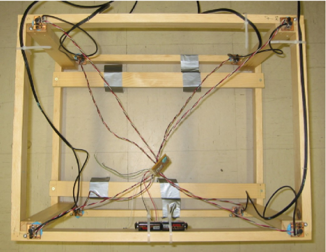
Figure 7: Top view of an array of 8 microphones mounted on a rectangular prism of dimensions 50 cm $\times$ 40 cm $\times$ 36 cm.

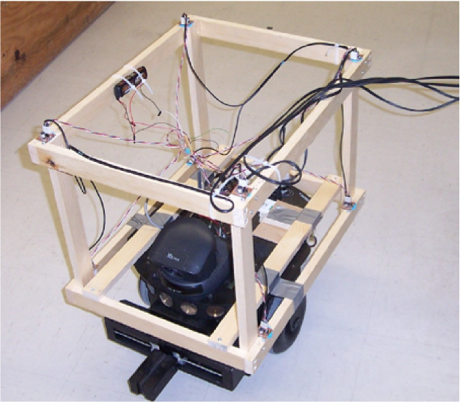
Figure 8: Microphone array installed on a Pioneer 2 robot.

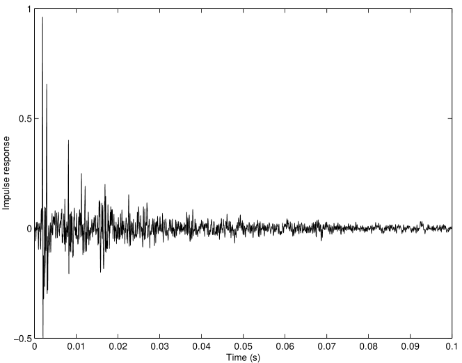
Figure 9: Impulse response of room reverberation. Secondary peaks represent reflections on the floor and on the walls.

The system was tested with sources placed in different locations in the environment. In each case, the distance and elevation are fixed and measures are taken for different horizontal angles. The mean angular error for each configuration is shown in Table 1. It is worth mentioning that part of this error, mostly at short distance, is due to the difficulty of accurately positionning the source and to the fact that the speaker used is not a point source. Other sources of error come from reverberation on the floor (more important when the source is high) and from the near-field approximation as shown in Figure 6. Overall, the angular error is the same regardless of the direction in the horizontal plane and varies only slightly with the elevation, due to the interference from floor reflections. This is an advantage over systems based on two microphones where the error is high when the source is located on the sides [4].

Table 1: Measured mean angular localization error

Distance, Elevation	Mean Angular Error
3 m, $-7^{\circ}$	$1.7^{\circ}$
3 m, $8^{\circ}$	$3.0^{\circ}$
1,5 m, $-13^{\circ}$	$3.1^{\circ}$
0,9 m, $24^{\circ}$	$3.3^{\circ}$

Unlike other works where the localization is performed actively during positioning [3], our approach is to localize the source before even moving the robot, which means that the source does not have to be continuous. In order to achieve that, the sound source localization system is disabled while the robot is moving toward the source. During a conversation between two or more persons, the robot alternates between the talkers. In presence of two simultaneous sources, the dominant one is naturally selected by the localization system. Figure 10 shows the experimental setup and images from the robot camera after localizing a source and moving its camera toward it. Most of the positionning error in the image is due to various actuator inaccuracies and the fact that the camera is not located exactly at the center of the array.

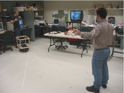
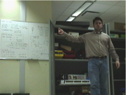
(a)                                    (b)

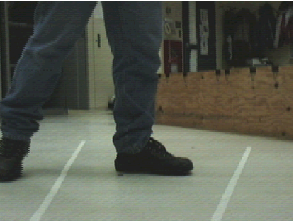
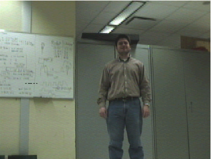
(c)                                    (d)

Figure 10: Photographs taken during experimentation. a) Experimental setup. b) Snapping fingers at a distance of $\sim 5\>\mathrm{m}$. c) Tapping foot at $\sim 2\>\mathrm{m}$. d) Speaking at a distance of $\sim 5\>\mathrm{m}$.

Experiments show that the system functions properly up to a distance between 3 and 5 meters, though this limitation is mainly a result of the noise and reverberation conditions in the laboratory. Also, not all sound types are equally well detected. Because of the whitening process explained in Section 2, each frequency has roughly the same importance in the cross-correlation. This means that when the sound to be localized is a tone, only a very small region of the spectrum contains useful information for the localization. The cross-correlation is then dominated by noise. This makes tones very hard to localize using the current algorithm. We also observed that this localization difficulty is present at a lesser degree for the human auditory system, which cannot accurately localize sinusoids in space.

On the other hand, some sounds are very easily detected by the system. Most of these sounds have a large bandwidth, like fricatives, fingers snapping, paper shuffling and percussive noises (object falling, hammer). For voice, the detection usually happens within the first two syllables.

5 Conclusion

Using an array of 8 microphones, we have implemented a system that accurately localizes sounds in three dimensions. Moreover, our system is able to perform localization even on short-duration sounds and does not require the use of any noise cancellation method. The precision of the localization is $3^{\circ}$ over 3 meters.

The TDOA estimation used in the system is shown to be relatively robust to noise and reverberation. Also, the algorithm for transforming the TDOA values to a direction is stable and independent of the speed of sound.

In its current form, the presented system still lacks some functionality. First, it cannot estimate the source distance. However, early simulations indicate that it would be possible to estimate the distance up to approximately 2 meters. Also, though possible in theory, the system is not yet capable of localizing two or more simultaneous sources and only the dominant one is perceived. In the case of more than one speaker, the “dominant sound source” alternates and it is possible to estimate the direction of both speakers.

References

- [1] A. Mahajan and M. Walworth. 3-d position sensing using the difference in the time-of-flights from a wave source to various receivers. IEEE Transactions on Robotics and Automation, 17(1):91–94, 2001.
- [2] Y. Matsusaka, T. Tojo, S. Kubota, K. Furukawa, D. Tamiya, K. Hayata, Y. Nakano, and T. Kobayashi. Multi-person conversation via multi-modal interface - a robot who communicate with multi-user. In Proceedings EUROSPEECH, pages 1723–1726, 1999.
- [3] K. Nakadai, T. Matsui, H. G. Okuno, and H. Kitano. Active audition system and humanoid exterior design. In Proceedings International Conference on Intelligent Robots and Systems, 2000.
- [4] K. Nakadai, H. G. Okuno, and H. Kitano. Real-time sound source localization and separation for robot audition. In Proceedings IEEE International Conference on Spoken Language Processing, pages 193–196, 2002.
- [5] H. G. Okuno, K. Nakadai, and H. Kitano. Social interaction of humanoid robot based on audio-visual tracking. In Proceedings of Eighteenth International Conference on Industrial and Engineering Applications of Artificial Intelligence and Expert Systems, pages 725–735, 2002.
- [6] M. Omologo and P. Svaizer. Acoustic event localization using a crosspower-spectrum phase based technique. In Proceedings IEEE International Conference on Acoustics, Speech, and Signal Processing, pages II–273–II–276, 1994.
- [7] Y. Zhang and J. Weng. Grounded auditory development by a developmental robot. In Proceedings INNS/IEEE International Joint Conference on Neural Networks, pages 1059–1064, 2001.