Onsager’s Cross Coupling Effects in Gas Flows Confined to Micro-channels

Abstract

In rarefied gases, mass and heat transport processes interfere with each other, leading to the mechano-caloric effect and thermo-osmotic effect, which are of interest to both theoretical study and practical applications. We employ the unified gas-kinetic scheme to investigate these cross coupling effects in gas flows in micro-channels. Our numerical simulations cover channels of planar surfaces and also channels of ratchet surfaces, with Onsager’s reciprocal relation verified for both cases. For channels of planar surfaces, simulations are performed in a wide range of Knudsen number and our numerical results show good agreement with the literature results. For channels of ratchet surfaces, simulations are performed for both the slip and transition regimes and our numerical results not only confirm the theoretical prediction [Phys. Rev. Lett. 107, 164502 (2011)] for Knudsen number in the slip regime but also show that the off-diagonal kinetic coefficients for cross coupling effects are maximized at a Knudsen number in the transition regime. Finally, a preliminary optimization study is carried out for the geometry of Knudsen pump based on channels of ratchet surfaces.

I Introduction

Onsager’s reciprocal relations for linear irreversible processes Onsager (1931a, b) play a crucial and important role in the theory of non-equilibrium thermodynamics. The kinetics of gases can be described by elementary processes of molecular collisions where microscopic reversibility and detailed balance are preserved. For systems slightly deviating from equilibrium, the linear response theory applies and Onsager’s reciprocal relations can be derived with the regression hypothesis Onsager (1931a). Typical examples in gas flows are the cross coupling between mass and heat diffusion in a multi-component gas Kremer (2010), and the mechano-caloric effect and thermo-osmotic effect in a single-component gas Waldmann (1967). The latter one not only provides an interesting case for theoretical study but also has practical applications in micro-devices Sone (2002); Aoki et al. (2006).

Waldmann Waldmann (1967) and Groot and Mazur de Groot and Mazur (1984) studied the cross coupling effect in channels of parallel planar surfaces in both the free molecular (${\rm Kn}\geq 10$) and slip ($0.001\leq{\rm Kn}\leq 0.1$) regimes. Loyalka Loyalka (1971, 1975) and Sharipov Sharipov (2006) analyzed the cross coupling effect by means of the linearized Boltzmann method and obtained the coupling coefficients numerically. Although the theoretical analysis of Loyalka Loyalka (1971) is valid for capillaries of arbitrary shape, most of the work, especially the numerical calculation Loyalka (1975); Sharipov and Seleznev (1998), was devoted to capillaries of planar surfaces or circular cross sections. The thermo-osmotic effect has attracted much attention recently since it can be used to design pumping devices without any moving part, i.e. the Knudsen pump Sone (2002). In addition to the earlier proposed Knudsen pump Sone (2002); Aoki et al. (2006), capillaries with ratchet surfaces have the potential for other possible configurations Würger (2011). The driving mechanism of these systems has been analyzed by Wüger Würger (2011) as well as Hardt et al. Hardt et al. (2013), and the mass and momentum transfer has been studied by Donkov et al. Donkov et al. (2011).

In the present work, we will study the cross coupling phenomena for a long capillary by using the unified gas-kinetic scheme Xu and Huang (2010); Huang et al. (2012). We will study the case of planar surfaces as well as the case of ratchet surfaces. The cross coupling mechanism will be presented for both cases. The coupling coefficients for the case of planar surfaces are numerically calculated and compared to literature results. The coupling coefficients for the case of ratchet surfaces are numerically calculated and analyzed, with a comparison to literature results as well. A preliminary geometry optimization for the design of Knudsen pump is also presented.

In our simulations for the case of ratchet surfaces, a channel of finite length is used with the pressure boundary condition applied at the two ends. In the presence of both pressure difference and temperature difference, the cross coupling effects, namely the mechano-caloric effect and thermo-osmotic effect, can be jointly studied to reveal the underlying reciprocal symmetry. However, with the periodic boundary condition used by Donkov et al.Donkov et al. (2011), only the thermo-osmotic effect is attainable because no pressure difference can be applied to generate the mechano-caloric effect. The numerical scheme used in the present work is applicable for all Knudsen numbers, and this allows us to study the cross coupling phenomena beyond the slip regime in which Wüger’s theory Würger (2011) is valid. In particular, we find that the cross coupling effects are maximized at a Knudsen number in the transition regime.

II Cross Coupling in Gas Flows in Micro-channels

In a closed system out of equilibrium, the rate of entropy production can be expressed as

$$\frac{dS}{dt}=\sum_{i=1}^{N}J_{i}X_{i},$$ (1)

where $S$ is the entropy, $J_{i}$ are the thermodynamic fluxes, and $X_{i}$ are the conjugate thermodynamic forces. For small deviation away from equilibrium, we have the linear relations between $J_{i}$ and $X_{i}$:

$$J_{i}=\sum_{j=1}^{N}L_{ij}X_{j},$$ (2)

where $L_{ij}$ are the kinetic coefficients. Onsager’s reciprocal relations state that $L_{ij}$ and $L_{ji}$ are equal as a result of microscopic reversibility Onsager (1931a, b); Gyarmati (1970). Starting from the Gibbs equation, the thermodynamic fluxes and forces can be identified for gas flows, and the corresponding constitutive equations can be derived Kremer (2010).

II.1 Micro-channels of planar surfaces

Figure 1: A schematic illustration of the cross coupling in a channel of planar surfaces.

A schematic illustration of the cross coupling in a channel of planar surfaces can be found in figure 1, where a long channel is confined by two parallel solid plates separated by a distance $H$ and connected with two reservoirs. The left reservoir is maintained at pressure $p_{0}-\Delta p/2$ and temperature $T_{0}-\Delta T/2$ while the right reservoir is maintained at $p_{0}+\Delta p/2$ and $T_{0}+\Delta T/2$. We use $\Delta p<0$ and $\Delta T>0$ in our simulations, with $|\Delta p/p_{0}|\ll 1$ and $|\Delta T/T_{0}|\ll 1$ to ensure the linear response. Usually, a mass flux to the right is generated by the pressure gradient due to $\Delta p<0$ and a heat flux to the left is generated by the temperature gradient due to $\Delta T>0$. For rarefied gas, however, $\Delta p$ also contributes to the heat flux and $\Delta T$ also contributes to the mass flux. These cross coupling effects are called the mechano-caloric effect and thermo-osmotic effect respectively.

For a single-component gas, the rate of entropy production can be expressed as Waldmann (1967)

$$\frac{dS}{dt}=J_{M}\Delta\left(-\frac{\nu}{T}\right)+J_{E}\Delta\left(\frac{1}{T}\right),$$ (3)

where $\nu$ is the chemical potential per unit mass, $J_{E}$ and $J_{M}$ are the energy flux and mass flux from the left reservoir to the right reservoir, and $\Delta$ means the quantity on the right minus the quantity on the left. Here $\nu$ and $J_{E}$ can be written as

$$\nu=h-Ts,$$ (4)

$$J_{E}=J_{Q}+hJ_{M},$$ (5)

where $s$ and $h$ are the entropy and enthalpy per unit mass, and $J_{Q}$ is the heat flux. Together with the Gibbs-Duhem equation

$$d\nu=-sdT+dp/\rho,$$ (6)

where $\rho$ is the mass density. Equation (3) becomes

$$\frac{dS}{dt}=-\frac{1}{\rho T}J_{M}\Delta p-\frac{1}{T^{2}}J_{Q}\Delta T.$$ (7)

According to equation (7), the thermodynamic forces and fluxes are connected in the form of

$$\begin{bmatrix}J_{M}\\ J_{Q}\end{bmatrix}=\begin{bmatrix}L_{MM}&L_{MQ}\\ L_{QM}&L_{QQ}\end{bmatrix}\begin{bmatrix}-\rho_{0}^{-1}T_{0}^{-1}\Delta p\\ -T_{0}^{-2}\Delta T\end{bmatrix},$$ (8)

with

$$L_{MQ}=L_{QM},$$ (9)

due to Onsager’s reciprocal relations. The detailed mechanism may vary with geometric configuration and rarefaction. Here and throughout the paper, the subscript ‘0’ denotes the reference state from which various deviations (in pressure, temperature, etc) are measured.

In the free molecular regime and with specular reflection on plates, the gas molecules travel ballistically from on side to the other and the distribution function at any point can be treated as a combination of two half-space maxwellians from the two reservoirs. The kinetic coefficients in equation (8) can be analytically derived in this case Waldmann (1967), given by

$$\begin{bmatrix}L_{MM}&L_{MQ}\\ L_{QM}&L_{QQ}\end{bmatrix}$$ (10)

$$=\frac{H\rho_{0}T_{0}}{4} \sqrt{\frac{8k_{B}T_{0}}{\pi m}}\begin{bmatrix}\rho_{0}/p_{0}&-1/2\\[5.0pt] -1/2&9p_{0}/4\rho_{0}\end{bmatrix}.$$

where $k_{B}$ is the Boltzmann constant and $m$ is the molecular mass.

If the temperature gradient is imposed on the plates and the gas molecules are diffusely reflected, then the mass flux due to the temperature gradient is generated by thermal creep on the plates de Groot and Mazur (1984); Sone (2002); Shen (2005). The kinetic coefficients in this case have been calculated by several authors using different methods Sharipov and Seleznev (1998). Assuming the length to height ratio of the channel is fixed and noting $\rho\lambda={\rm constant}$ and $\mu\propto\rho^{0}T^{1/2}$ for hard-sphere molecules, the average velocity $\overline{U}$ induced by thermal creep can be estimated from the Maxwell slip boundary condition Shen (2005),

$$\overline{U}\sim\frac{\mu_{0}}{\rho_{0}T_{0}}\nabla T\propto{\rm Kn}\frac{\Delta T}{\sqrt{T_{0}}},$$ (11)

where $\lambda$ is the mean free path, $\mu$ is the dynamic viscosity independent of the density, and ${\rm Kn}=\lambda_{0}/H$ is the Knudsen number. In later sections, we will show that $L_{MQ}$ and $L_{QM}$ are equal and increase with the increasing ${\rm Kn}$.

II.2 Micro-channels of ratchet surfaces

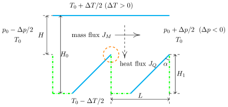
(a)

(b)

Figure 2: A schematic illustration of the cross coupling in a channel of ratchet surfaces. (a) Two blocks of a channel of ratchet surfaces. The upper wall and the lower tilted walls (blue solid lines) are diffusely reflective. The lower horizontal and vertical walls (green dot-dashed lines) are specularly reflective. (b) Simulation geometry with multiple blocks in the channel.

The mechanism for the cross coupling in a channel of ratchet surfaces is more complicated. Consider a long channel consisting of repeating structure Donkov et al. (2011) as shown in figure 2a, where the two ends are connected to two reservoirs maintained at $(p_{0}-\Delta p/2,T_{0})$ on the left and $(p_{0}+\Delta p/2,T_{0})$ on the right with $\Delta p<0$. The upper wall (blue solid lines) is diffusely reflective and maintained at $T_{0}+\Delta T/2$ with $\Delta T>0$, and the lower tilted walls (blue solid lines) are diffusely reflective and maintained at $T_{0}-\Delta T/2$. The lower horizontal and vertical walls (green dot-dashed lines) are specularly reflective. Usually, a mass flux from the left to the right is generated by the pressure gradient due to $\Delta p<0$, and a heat flux from the top to the bottom is generated by the temperature gradient due to $\Delta T>0$. For rarefied gas, however, $\Delta p$ also contributes to the vertical heat flux and $\Delta T$ also contributes to the horizontal mass flux. Our simulations are carried out for $|\Delta p/p_{0}|\ll 1$ and $|\Delta T/T_{0}|\ll 1$ to ensure the linear response.

In general, a temperature difference can also be applied in the horizontal direction and a heat flux can also exist in this direction as the conjugate flux. This means that there are three thermodynamic forces (i.e. the pressure difference in the horizontal direction, the temperature difference in the horizontal direction, and the temperature difference in the vertical direction) and their conjugate fluxes. In the present study, we set the temperature difference in the horizontal direction to be zero. We also ignore the heat flux in the horizontal direction (although it may well exist). As a result, the two thermodynamic forces and their conjugate fluxes under consideration are connected in the form of

$$\begin{bmatrix}J_{M}\\ J_{Q}\end{bmatrix}=\begin{bmatrix}L_{MM}&L_{MQ}\\ L_{QM}&L_{QQ}\end{bmatrix}\begin{bmatrix}-\rho_{0}^{-1}T_{0}^{-1}\Delta p\\ -T_{0}^{-2}\Delta T\end{bmatrix},$$ (12)

with

$$L_{MQ}=L_{QM},$$ (13)

due to Onsager’s reciprocal relations. Here $J_{M}$ is the horizontal mass flux (from the left to the right) and $J_{Q}$ is the vertical heat flux (from the bottom to the top).

Since the upper wall and the lower tilted walls are maintained at different temperatures (with $\Delta T>0$), the isothermal lines near the tips of the tilted walls (indicated by a red dashed circle) are sharply curved and a thermal edge flow is induced at the tip from the top to the bottom Sone (2002); Hardt et al. (2013). It is possible to make a rough estimation of the induced flow velocity at the tip Sone (2002); Würger (2011). If all the walls are assumed to be diffusely reflective, then the temperature gradient along the tilted wall near the tip is approximated by

$$\nabla_{||}T=\Delta T\frac{\pi^{2}}{(2\pi-\alpha)^{2}}\cos\left(\frac{\alpha}{2}\right)\frac{H^{-\pi/(2\pi-\alpha)}}{\lambda_{0}^{1-\pi/(2\pi-\alpha)}},$$ (14)

where $\lambda_{0}$ is the mean free path at $(p_{0},T_{0})$ Würger (2011). By use of $\rho\lambda={\rm constant}$ and $\mu\propto\rho^{0}T^{1/2}$ for hard-sphere molecules, the induced velocity in the slip regime can be estimated from the slip boundary condition Shen (2005):

$${\overline{U}}\sim \frac{\mu_{0}}{\rho_{0}T_{0}}\nabla_{||}T$$ (15)

$$\propto \frac{\Delta T}{\sqrt{T_{0}}}\frac{1}{(2\pi-\alpha)^{2}}\cos\left(\frac{\alpha}{2}\right)\left(\frac{\lambda_{0}}{H}\right)^{\pi/(2\pi-\alpha)}.$$

For $0\leq\alpha<\pi/2$ and ${\rm Kn}=\lambda_{0}/H<1$ in the slip regime, the induced velocity is

1. proportional to $\Delta T$,

2. a decreasing function of $T_{0}$,

3. a decreasing function of $\alpha$ because a smaller $\alpha$ means sharper edges,

4. an increasing function of ${\rm Kn}$ because a larger ${\rm Kn}$ leads to stronger non-equilibrium effect.

It is worth noting that $\overline{U}$ will decrease if the Knudsen number exceeds a certain value since the thermally induced flows are typically strongest in the lower transition regime (where the Knudsen number is slightly higher than that in the slip regime) Sone (2002). For the current configuration, the average velocity can be expressed as

$$\overline{U}\propto{\rm Kn}^{C_{2}}\frac{\Delta T}{\sqrt{T_{0}}},$$ (16)

where $C_{2}$ is a constant determined by a specific geometry.

III Numerical Results and Discussion

The kinetic coefficients are to be calculated and presented in dimensionless form as

$${\hat{L}}_{MQ} =-L_{MQ}\left(\frac{2k_{B}}{m\rho_{0}C_{0}^{3}H}\right),$$ (17)

$${\hat{L}}_{QM} =-L_{QM}\left(\frac{2k_{B}}{m\rho_{0}C_{0}^{3}H}\right),$$

where $\rho_{0}$ and $T_{0}$ are the density and temperature of the reference state, $C_{0}=\sqrt{2k_{B}T_{0}/m}$ is the most probable speed, and $H$ is the height of the channel to define the Knudsen number ${\rm Kn}=\lambda_{0}/H$. The mean free path in the reference state is $\lambda_{0}$. The above normalization makes it easier to compare our results with the benchmark solutions, and the normalized coefficients can reflect the mechanism more directly as shown below.

As the density variation is small in the simulation, the mass flux can be expressed as

$$J_{M}\approx\rho_{0}\overline{U}H.$$ (18)

Assuming that there is no pressure difference, we have

$$\rho_{0}\overline{U}H={\hat{L}}_{MQ}\left(\frac{m\rho_{0}C_{0}^{3}H}{2k_{B}}\right)\frac{\Delta T}{T_{0}^{2}},$$ (19)

which leads to

$$\overline{U}={\hat{L}}_{MQ}C_{0}\frac{\Delta T}{T_{0}}\propto{\hat{L}}_{MQ}\frac{\Delta T}{\sqrt{T_{0}}}.$$ (20)

Through a comparison of equation (20) with equations (11) and (16), the dimensionless ${\hat{L}}_{MQ}$ is expected to have the form

$${\hat{L}}_{MQ}=C_{1}{\rm Kn}^{C_{2}},$$ (21)

where $C_{1}$ and $C_{2}$ are constants determined by a specific geometry. They are to be obtained by fitting the simulation data.

For the cross coupling considered here, two thermodynamic fluxes (mass flux and heat flux) and the corresponding forces (pressure difference and temperature difference) can be directly extracted from the simulation data in a single simulation. In order to determine all the kinetic coefficients, simulations need to be performed (at least) twice with different $\Delta p$ and $\Delta T$ for the same system (with the same geometry and the same Knudsen number).

III.1 Cross coupling in channels of planar surfaces

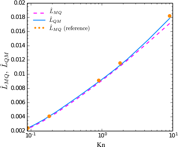
Figure 3: The normalized off-diagonal coefficients ${\hat{L}}_{MQ}$ and ${\hat{L}}_{QM}$ versus the Knudsen number. The reference is the S-model solution based on the variational method by Chernyak et al. Chernyak et al. (1979).

First we calculate the kinetic coefficients for channels with planar surfaces and compare our results with those in literature Sharipov and Seleznev (1998); Chernyak et al. (1979); Cercignani (1988). A schematic illustration for the simulation geometry can be found in figure 1. The solid surfaces are diffusely reflective and have linearly distributed temperature from $T_{0}-\Delta T/2$ to $T_{0}+\Delta T/2$. The gas particles are hard-sphere and monatomic, with the Prandtl number ${\rm Pr}=2/3$ and the dynamic viscosity $\mu\propto T^{0.5}$. The Knudsen number is defined as ${\rm Kn}=\lambda_{0}/H$. $\Delta p$ and $\Delta T$ are kept small enough so that the response of fluxes to forces is linear. The length to height ratio of the channel is taken to be $20$ in order to reduce the influence of inlet and outlet. When extracting the kinetic coefficients, the pressure and temperature differences are measured at the inlet and outlet, the mass flux $J_{M}$ is measured over the cross section at the inlet and outlet, and the heat flux $J_{Q}$ is measured over the cross section in the middle of the channel.

Figure 3 shows the normalized off-diagonal coefficients ${\hat{L}}_{MQ}$ and ${\hat{L}}_{QM}$ versus the Knudsen number. The two coefficients are very close to each other with a relative difference less than $5\%$, and have good agreement with the S-model solution based on the variational method by Chernyak et al. Chernyak et al. (1979). The off-diagonal coefficients are zero at ${\rm Kn}=0$ since there is no thermally induced flow in the continuum limit and the heat flux simply follows Fourier’s law. The normalized coefficients increase with the increasing Knudsen number. In the slip regime ($0.001<{\rm Kn}<0.1$), ${\hat{L}}_{MQ}\sim{\rm Kn}$, while at large Knudsen numbers (${\rm Kn}>3$), the profile is almost linear, which means ${\hat{L}}_{MQ}={\hat{L}}_{QM}\sim\log({\rm Kn})$. This agrees with the conclusion obtained from linearized Boltzmann equation for two-dimensional infinitely long channels Cercignani (1988); Sharipov and Seleznev (1998).

III.2 Cross coupling in channels of ratchet surfaces

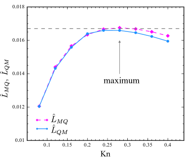
(a)

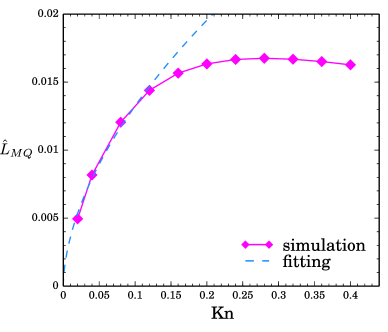
(b)

Figure 4: (a) The normalized off-diagonal coefficients ${\hat{L}}_{MQ}$ and ${\hat{L}}_{QM}$ versus the Knudsen number. The dashed line is used to indicate that ${\hat{L}}_{MQ}$ and ${\hat{L}}_{QM}$ both exhibit their maxima at ${\rm Kn}\approx 0.28$. (b) ${\hat{L}}_{MQ}$ from simulations. For ${\rm Kn}\leq 0.12$, the data fitting gives ${\hat{L}}_{MQ}=0.0483{\rm Kn}^{0.562}$, represented by the dashed line.

In our simulations, each channel consists of seven repeating blocks as shown in figure 2a and each block has $L/H_{0}=1$, $H_{1}/H=1$, and $\alpha=45^{\circ}$. In addition, two parallel sections with specularly reflective walls of length $L$ are attached at the two ends. The channel is then connected to two reservoirs. A schematic illustration for the whole system is shown in figure 2b. The parallel sections with specularly reflective walls connected to the reservoirs are introduced to reduce the boundary effect of the inlet/outlet on the ratchet sections and to simplify the measurement of mass flux. The gas particles are still hard-sphere and monatomic, with the Prandtl number ${\rm Pr}=2/3$ and the dynamic viscosity $\mu\propto T^{0.5}$. The Knudsen number is defined as ${\rm Kn}=\lambda_{0}/H$. When extracting the kinetic coefficients, the pressure difference is measured at the inlet and outlet, the mass flux $J_{M}$ is measured over the cross section at the inlet and outlet, and the heat flux $J_{Q}$ is measured over all the lower tilted walls.

Figure 4a shows the normalized off-diagonal coefficients ${\hat{L}}_{MQ}$ and ${\hat{L}}_{QM}$ versus the Knudsen number. The two coefficients are very close to each other with a relative difference less than $2\%$, indicating that the relation $L_{MQ}=L_{QM}$ is well satisfied in our simulations. The off-diagonal coefficients are zero at ${\rm Kn}=0$ since there is no thermally induced flow in the continuum limit and the heat flux simply follows Fourier’s law. As the Knudsen number increases from zero, the rarefaction effects begin to emerge at the sharp edge of the ratchet and lead to nonzero ${\hat{L}}_{MQ}$ and ${\hat{L}}_{QM}$. It is further noted that ${\hat{L}}_{MQ}$ and ${\hat{L}}_{QM}$ both exhibit their maxima at ${\rm Kn}\approx 0.28$. This value of ${\rm Kn}$ (in the transition regime) is consistent with the results for ${\hat{L}}_{MQ}$ in Ref. Donkov et al. (2011) for a similar ratchet geometry with periodic boundary condition. Physically, the cross coupling effects arise from the thermally induced flow, which is the strongest at the sharp edge. As the Knudsen number becomes higher than a certain value, the surface structure is no longer clearly detectable by the particles, and hence the off-diagonal coefficients will decrease with the increasing Knudsen number. From the distinct behaviors of ${\hat{L}}_{MQ}$ as a function of ${\rm Kn}$ in the slip and transition regimes, a maximum is expected for ${\hat{L}}_{MQ}$.

Now we perform the data fitting according to $L_{MQ}=L_{QM}$ and equation (21). Since this formula is valid in the slip regime ($0.001\leq{\rm Kn}\leq 0.1$), two additional simulations are carried out to obtain ${\hat{L}}_{MQ}$ at ${\rm Kn}=0.02$ and $0.04$, as shown in figure 4b. The data fitting uses only the first four data points (for ${\rm Kn}\leq 0.12$, see figure 4b) and gives

$${\hat{L}}_{MQ}=0.0483{\rm Kn}^{0.562}.$$ (22)

Inserting $\alpha=\pi/4$ into equation (15), we find

$${\bar{U}}\propto{\rm Kn}^{4/7},$$ (23)

in which the exponent $4/7\simeq 0.571$ is very close to the fitting parameter ${0.562}$ in equation (22). Physically, the exponent $C_{2}$ directly reflects the underlying cross coupling mechanism, and therefore our simulation results have confirmed the theory proposed in Ref. Würger (2011) for ${\rm Kn}$ in the slip regime.

IV Knudsen Pump

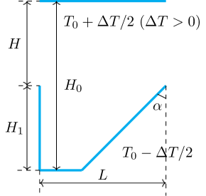
(a)

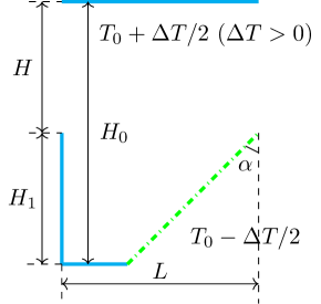
(b)

Figure 5: (a) The diffuse configuration. (b) The diffuse-specular configuration.

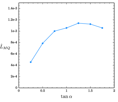
(a)

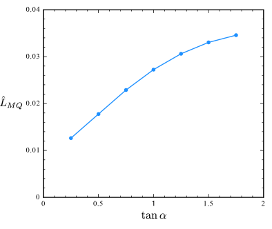
(b)

Figure 6: ${\hat{L}}_{MQ}$ plotted as a function of $\tan\alpha$ for $L/H=2$, $H_{1}/H=1$, and ${\rm Kn}=0.28$. (a) ${\hat{L}}_{MQ}$ in the diffuse configuration. (b) ${\hat{L}}_{MQ}$ in the diffuse-specular configuration.

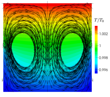
(a)

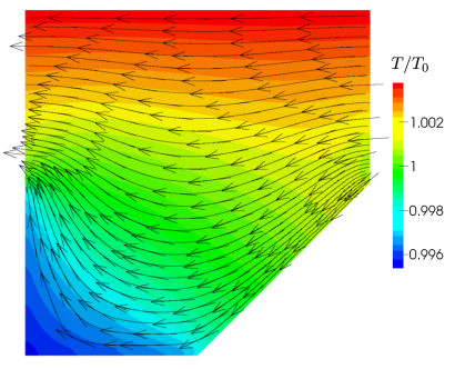
(b)

Figure 7: The temperature distribution and streamlines plotted in one block with the periodic boundary condition. (a) The diffuse configuration with $\alpha=0$. (b) A typical diffuse-specular configuration.

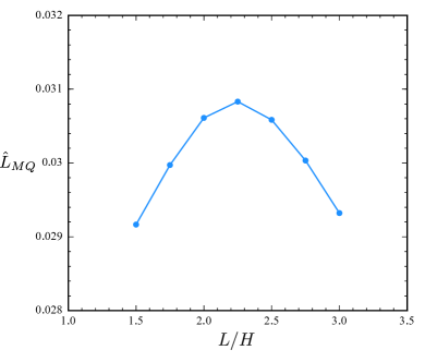
(a)

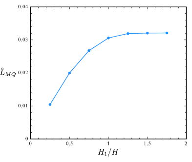
(b)

Figure 8: ${\hat{L}}_{MQ}$ in the diffuse-specular configuration. (a) ${\hat{L}}_{MQ}$ plotted as a function of $L/H$ for $\tan\alpha=1.25$, $H_{1}/H=1$, and ${\rm Kn}=0.28$. (b) ${\hat{L}}_{MQ}$ plotted as a function of $H_{1}/H$ for $\tan\alpha=1.25$, $L/H=2.5$, and ${\rm Kn}=0.28$.

Wüger Würger (2011) and Donkov et al. Donkov et al. (2011) have proposed the capillary with ratchet surfaces as another possible configuration for Knudsen pump. In this section, a preliminary optimization study is provided for this purpose. For accuracy and simplicity, only one block is used in the simulations here and the inlet/outlet is replaced by the periodic boundary condition, which is suitable for the computation of ${\hat{L}}_{MQ}$. The upper wall is still diffusely reflective, but the lower walls now have two different configurations (as shown in figure 5):

• All the lower walls are diffusely reflective. This is referred to as the diffuse configuration.

• The lower horizontal and vertical walls are diffusely reflective, and the lower tilted walls are specularly reflective. This is referred to as the diffuse-specular configuration, the same as that adopted in Ref. Donkov et al. (2011).

Technically, these two configurations are compatible with the periodic boundary condition applied here, under which only the thermo-osmotic effect is attainable and the coefficient ${\hat{L}}_{MQ}$ can be computed. As to the configuration shown in figure 2a, it is suitable for the application of pressure difference, under which the mechano-caloric effect coexists with the thermo-osmotic effect and hence ${\hat{L}}_{QM}$ and ${\hat{L}}_{MQ}$ can be computed simultaneously to verify the reciprocal symmetry.

Figure 6 shows ${\hat{L}}_{MQ}$ as a function of $\tan\alpha$ for $L/H=2$, $H_{1}/H=1$, and ${\rm Kn}=0.28$. The left panel in the figure is for the diffuse configuration and the right panel is for the diffuse-specular configuration. In the diffuse configuration, the thermally induced flows arise on both sides of the sharp edge and the net flow is consequently diminished Hardt et al. (2013). This explains the very small magnitude of ${\hat{L}}_{MQ}$ in figure 6a. In fact, if $\alpha=0$, then there will be no net mass flow in the $x$ direction because two identical vortices are formed between the ‘needles’ as shown in figure 7a. The optimal value of $\alpha$ (at which ${\hat{L}}_{MQ}$ is maximized) is approximately given by $\tan\alpha=1.25$. In the diffuse-specular configuration, the thermally induced flow occurs only on the diffusely reflective surfaces, and therefore the net mass flow is much higher than that in the diffuse configuration. The temperature distribution and streamlines of a typical diffuse-specular configuration are shown in figure 7b, and they are similar to the corresponding results in Ref. Donkov et al. (2011). In this case, figure 6b shows ${\hat{L}}_{MQ}$ to be an increasing function of $\tan\alpha$. For $L/H$ and $H_{1}/H$ used here, $\tan\alpha$ varies between $0$ and $2$. At a larger $\alpha$, the flow explores a smaller region between the vertical and tilted walls, with the streamlines showing less change in direction. This means the flow is less dissipated and the thermo-osmotic effect is stronger.

Now we focus on the diffuse-specular configuration. Figure 8a shows ${\hat{L}}_{MQ}$ as a function of $L/H$ for $\tan\alpha=1.25$, $H_{1}/H=1$, and ${\rm Kn}=0.28$. It is seen that ${\hat{L}}_{MQ}$ is maximized at $L/H\approx 2.25$. Here $L/H$ can increase from $1.25$ to $\infty$. When $L/H$ is close to $1.25$, the flow changes greatly in direction at the lower left corner, and hence the density of dissipation is large. On the other hand, when $L/H$ is very large, the total dissipation is also large because of the large space involved. As a consequence, an optimal value of $L/H$ is expected at which the total dissipation is minimized and ${\hat{L}}_{MQ}$ is maximized. Figure 8b shows the ${\hat{L}}_{MQ}$ as a function of $H_{1}/H$ for $\tan\alpha=1.25$, $L/H=2.5$, and ${\rm Kn}=0.28$. Here $H_{1}/H$ varies between $0$ and $2$. It is seen that ${\hat{L}}_{MQ}$ is an increasing function of $H_{1}/H$ and saturates at $H_{1}/H\approx 1.25$. This is expected because the thermally induced flow is only appreciable within a certain distance to the edge. For $H_{1}$ below this distance, ${\hat{L}}_{MQ}$ increases with the increasing $H_{1}$, while for $H_{1}$ above this distance, ${\hat{L}}_{MQ}$ saturates.

V Concluding remarks

The mechano-caloric effect and thermo-osmotic effect in a single-component gas not far away from equilibrium have been investigated. The mechanisms for micro-channels with planar surfaces and ratchet surfaces have been analyzed. Numerical simulations have been performed to compute the off-diagonal kinetic coefficients for the cross coupling effects as a function of the Knudsen number. For channels with planar surfaces, our simulation results have been compared with the S-model solution of Chernyak et al. Chernyak et al. (1979), showing good agreement for $0.1<{\rm Kn}<10$. For channels with ratchet surfaces, our simulations have been performed for both the slip and transition regimes. The theoretical prediction for micro-channels with ratchet surfaces in the slip regime, which gives $\overline{U}\propto{\hat{L}}_{MQ}\propto{\rm Kn}^{C}$, has been numerically checked, showing good agreement with our simulation results. It has also been shown that ${\hat{L}}_{MQ}$ and ${\hat{L}}_{QM}$ both exhibit their maxima at ${\rm Kn}\approx 0.28$ in the transition regime, as anticipated theoretically.

For both types of channels, our simulation results for the off-diagonal kinetic coefficients have confirmed Onsager’s reciprocal relation. Given the fundamental importance of reciprocal symmetry in non-equilibrium thermodynamics, we want to point out that (i) our simulation geometry for channels of ratchet surfaces allows the coexistence of the mechano-caloric and thermo-osmotic effects, (ii) this coexistence makes the numerical verification of reciprocal symmetry possible, and (iii) this verification shows that thermodynamic consistency is ensured in our simulation approach based on the unified gas-kinetic scheme Xu and Huang (2010); Huang et al. (2012). Here we remark that the reciprocal symmetry has been observed in the slip regime and beyond. This is physically acceptable because small pressure and temperature differences have been used in our simulations to ensure that dynamics is slow and hence linear response is valid even if the Knudsen number is not very small.

Since micro-channels with ratchet surfaces have the potential to be an alternative configuration of Knudsen pump, a preliminary optimization study has been carried out for its geometry. Two different configurations have been used for this purpose — (i) the diffuse configuration in which all the lower walls are diffusely reflective, and (ii) the diffuse-specular configuration in which the lower horizontal and vertical walls are diffusely reflective and the lower tilted walls are specularly reflective. It turns out that the diffuse-specular configuration leads to a much stronger thermo-osmotic effect (by an order of magnitude). In particular, we have measured the off-diagonal coefficient ${\hat{L}}_{MQ}$ as a function of various geometrical parameters, and our results can be used to help optimize the pump design.

Appendix A Simulation Method: Unified Gas-kinetic Scheme

The unified gas-kinetic scheme (UGKS) is a multi-scale method based on the kinetic equation, which can be used for simulating flows of all Knudsen numbers Xu and Huang (2010); Huang et al. (2012).

The BGK-type equation in one spatial dimension without external force is given by

$$\frac{\partial f}{\partial t}+u\frac{\partial f}{\partial x}=Q(f),\quad Q(f)=\frac{f^{+}-f}{\tau},$$ (24)

where $f(x,t,{\bf u})$ is the velocity distribution function at $(x,t)$, ${\bf u}=(u,v,w)$ is the particle velocity, $f^{+}$ is the post-collision distribution function, and $\tau$ is the relaxation time. In the finite-volume framework, the evolution of the distribution function and conservative variables in the $i$-th cell are given by

$$f_{i}^{n+1}=f_{i}^{n}- \frac{1}{\Delta x}\int_{t^{n}}^{t^{n+1}}u(f_{i+1/2}-f_{i-1/2})dt$$ (25)

$$+ \frac{\Delta t}{2}(Q_{i}^{n}+Q_{i}^{n+1}),$$

and

$${\bf W}_{i}^{n+1}={\bf W}_{i}^{n}-\frac{1}{\Delta x}\int_{t^{n}}^{t^{n+1}}\int\psi u(f_{i+1/2}-f_{i-1/2})d{\bf u}dt,$$ (26)

where ${\bf W}=(\rho,\rho U,\rho E)^{T}$, $\psi=(1,u,{\bf u}^{2}/2)^{T}$, $U$ is the macroscopic velocity, $E$ is the total energy density, and $d{\bf u}=dudvdw$.

The construction of the interface flux is the key to UGKS. Assuming an interface is located at $x=0$, the accurate time evolution of the distribution function at the interface from $t^{n}=0$ to $t^{n+1}=\Delta t$ is described by the solution of the BGK-type equation along the characteristics,

$$f(0,t,{\bf u})= \frac{1}{\tau}\int_{0}^{t}f^{+}(-u(t-t^{\prime}),t^{\prime},{\bf u})e^{-(t-t^{\prime})/\tau}dt^{\prime}$$ (27)

$$+ e^{-t/\tau}f_{0}(-ut,{\bf u}),$$

where $f_{0}$ is the initial distribution function at $t=0$. Here $f_{0}$ is assumed to be linearly distributed within each cell and discontinuous at the interface, given by

$$f_{0}=(f_{0}^{L}+xf_{x}^{L})(1-H[x])+(f_{0}^{R}+xf_{x}^{R})H[x],$$ (28)

where $f_{0}^{L}$ and $f_{0}^{R}$ are the reconstructed distribution functions at both sides of the cell interface, $f_{x}^{L}$ and $f_{x}^{R}$ are the corresponding derivatives, and $H[x]$ is the Heaviside function. The post-collision term $f^{+}$ is approximated by the first-order Taylor expansion on both sides of the interface, given by

$$f^{+}=f^{+}_{0}+g_{0}\left[(1-H[x])a^{L}x+H[x]a^{R}x+At\right],$$ (29)

where $g_{0}$ is the Maxwell distribution which is uniquely determined by ${\bf W}_{0}$,

$${\bf W}_{0}=\int(f_{0}^{L}H[u]+f_{0}^{R}(1-H[u]))\psi d{\bf u}.$$ (30)

The coefficients $a^{L}$, $a^{R}$, and $A$ are computed via the partial derivatives of the conservative variables at $(x,t)=(0,0)$, for example,

$$a^{L}=\frac{1}{g_{0}}\left(\frac{\partial g_{0}}{\partial{\bf W}_{0}}\right){\bf W}_{x}^{L}\approx\frac{1}{g_{0}}\left(\frac{\partial g_{0}}{\partial{\bf W}_{0}}\right)\frac{{\bf W}^{L}-{\bf W}_{0}}{x^{L}},$$ (31)

where ${\bf W}^{L}$ is the conservative variables at the left cell, and $x^{L}$ is the coordinate of the left cell center. The time derivative part $A$ is computed via

$${\bf W}_{t}=-\int(a^{L}H[u]+a^{R}(1-H[u]))ug_{0}\psi d{\bf u}.$$ (32)

In the present work, $f^{+}$ takes the form from the BGK-Shakhov model Shakhov (1972) to result in a realistic Prandtl number and the relaxation time is $\tau=\mu/p$.

References

- Onsager (1931a) L. Onsager, Phys. Rev. 37, 405 (1931a).
- Onsager (1931b) L. Onsager, Phys. Rev. 38, 2265 (1931b).
- Kremer (2010) G. M. Kremer, An Introduction to the Boltzmann Equation and Transport Processes in Gases (Springer-Verlag Berlin Heidelberg, 2010) pp. 1–310.
- Waldmann (1967) L. Waldmann, Z. Naturforsch. 22, 1269 (1967).
- Sone (2002) Y. Sone, Kinetic Theory and Fluid Dynamics (Springer, 2002) pp. 1–353.
- Aoki et al. (2006) K. Aoki, P. Degond, and L. Mieussens, in 25th International Symposium on Rarefied Gas Dynamics (Saint-Petersburg, Russia, 2006) pp. 1–6.
- de Groot and Mazur (1984) S. R. de Groot and P. Mazur, Non-Equilibrium Thermodynamics (Dover Publications, 1984) pp. 1–510.
- Loyalka (1971) S. K. Loyalka, J. Chem. Phys. 55, 4497 (1971).
- Loyalka (1975) S. K. Loyalka, J. Chem. Phys. 63, 4054 (1975).
- Sharipov (2006) F. Sharipov, Phys. Rev. E 73, 026110 (2006).
- Sharipov and Seleznev (1998) F. Sharipov and V. Seleznev, J. Phys. Chem. Ref. Data 27, 657 (1998).
- Würger (2011) A. Würger, Phys. Rev. Lett. 107, 164502 (2011).
- Hardt et al. (2013) S. Hardt, S. Tiwari, and T. Baier, Phys. Rev. E 87, 063015 (2013).
- Donkov et al. (2011) A. A. Donkov, S. Tiwari, T. Liang, S. Hardt, A. Klar, and W. Ye, Phys. Rev. E 84, 016304 (2011).
- Xu and Huang (2010) K. Xu and J.-C. Huang, J. Comput. Phys. 229, 7747 (2010).
- Huang et al. (2012) J.-C. Huang, K. Xu, and P. Yu, Commun. Comput. Phys. 12, 662 (2012).
- Gyarmati (1970) I. Gyarmati, Non-equilibrium Thermodynamics – Field Theory and Variational Principles (Springer, 1970).
- Shen (2005) C. Shen, Rarefied Gas Dynamics: Fundamentals, Simulations and Micro Flows (Springer, 2005) p. 421.
- Chernyak et al. (1979) V. G. Chernyak, V. V. Kalinin, and P. E. Suetin, J. Eng. Phys. 36, 696 (1979).
- Cercignani (1988) C. Cercignani, The Boltzmann Equation and Its Applications (Springer New York, 1988) pp. 1–456.
- Shakhov (1972) E. M. Shakhov, Fluid Dyn. 3, 95 (1972).