On forbidden induced subgraphs for unit disk graphs

Abstract

A unit disk graph is the intersection graph of disks of equal radii in the plane. The class of unit disk graphs is hereditary, and therefore admits a characterization in terms of minimal forbidden induced subgraphs. In spite of quite active study of unit disk graphs very little is known about minimal forbidden induced subgraphs for this class. We found only finitely many minimal non unit disk graphs in the literature. In this paper we study in a systematic way forbidden induced subgraphs for the class of unit disk graphs. We develop several structural and geometrical tools, and use them to reveal infinitely many new minimal non unit disk graphs. Further we use these results to investigate structure of co-bipartite unit disk graphs. In particular, we give structural characterization of those co-bipartite unit disk graphs whose edges between parts form a $C_{4}$-free bipartite graph, and show that bipartite complements of these graphs are also unit disk graphs. Our results lead us to propose a conjecture that the class of co-bipartite unit disk graphs is closed under bipartite complementation.

1 Introduction

A graph is unit disk graph (UDG for short) if its vertices can be represented as points in the plane such that two vertices are adjacent if and only if the corresponding points are at distance at most 1 from each other. Unit disk graphs has been very actively studied in recent decades. One of the reasons for this is that UDGs appear to be useful in number of applications. Perhaps a major application area for UDGs is wireless networks. Here a UDG is used to model the topology of a network consisting of nodes that communicates by means of omnidirectional antennas with equal transmission-reception range. Many research projects aimed at designing algorithms for different graph optimization problems specifically on unit disk graphs, as solutions to these problems are of practical importance for efficient operation of modeled networks. We refer the reader to [2, 3] and references therein for more details on applications of UDGs.

The class of unit disk graphs is hereditary, that is closed under vertex deletion or, equivalently, closed under induced subgraphs. It is well known and can be easily proved that every hereditary class of graphs admits characterization in terms of minimal forbidden induced subgraphs. Formally, for a hereditary class $\mathcal{X}$ there exists a unique minimal under inclusion set of graphs $M$ such that $\mathcal{X}$ coincides with the family $Free(M)$ of graphs none of which contains a graph from $M$ as an induced subgraph. Graphs in $M$ are called minimal forbidden induced subgraphs for $\mathcal{X}$. Such an obstructive specification of a hereditary class may be useful for investigation of its structural, algorithmic and combinatorial properties. For instance, forbidden subgraphs characterization of a class may be helpful in testing whether a graph belongs to the class or not. In particular, if the set of minimal forbidden subgraphs is finite, then, clearly, the problem of recognizing graphs in the class is polynomially solvable. However, describing a hereditary class in terms of its minimal forbidden induced subgraphs may be extremely hard problem. For example, for the class of perfect graphs it took more than 40 years to obtain forbidden subgraph characterization [5].

Despite extensive study of the class of unit disk graphs very little is known about its forbidden induced subgraphs. We found only few minimal non unit disk graphs in the literature, namely, $K_{1,6}$, $K_{2,3}$, and five other graphs (see Figure 1) [10, 11]. However, unless $\textup{P}=\textup{NP}$, the set of minimal forbidden induced subgraphs is infinite, since the problem of recognizing unit disk graphs is known to be NP-hard [4]. Interestingly, only the fact that unit disk graphs avoid $K_{1,6}$ already turned out to be useful in algorithms design. For example, the fact was utilized in [13] for obtaining 3-approximation algorithm for the maximum independent set problem and 5-approximation algorithm for the dominating set problem. In [7] da Fonseca et al. used additional geometrical restrictions of UDGs to design an algorithm for the latter problem with better approximation factor $44/9$. The authors pointed out that further improvement may require new information about forbidden induced subgraphs for UDGs, and in a subsequent paper [8] they developed algorithm for recognizing UDGs. Unfortunately, (though, not surprising as the corresponding problem is NP-hard) in worst cases the algorithm works exponential time, and the experimental results are available only for small graphs and do not discover any new minimal forbidden subgraphs.

In the present paper we systematically study forbidden induced subgraphs for the class of unit disk graphs, and reveal infinitely many new minimal forbidden subgraphs. For example, we show that all complements of even cycles with at least eight vertices are minimal non-UDGs. In contrast, all complements of odd cycles are UDGs. We use the obtained results to investigate structure of co-bipartite unit disk graphs. Specifically, we characterize the class of $C_{4}^{*}$-free co-bipartite UDGs, that is co-bipartite UDGs whose edges between parts form a bipartite graph without cycle on four vertices. Further we show that bipartite complement of every $C_{4}^{*}$-free co-bipartite UDG is also (co-bipartite) UDG. This fact and the structure of the set of found obstructions leads us to pose a conjecture that the class of co-bipartite UDGs is closed under bipartite complementation.

The paper is organized as follows. In Section 2 we introduce necessary definitions and notation. In Section 3 we develop auxiliary geometrical and structural tools that may be of their own interest. Using these tools we derive new minimal forbidden induced subgraphs in Section 4. In Section 5 we give structural characterization of certain classes of co-bipartite UDGs. In the last Section 6 we discuss the results and open problems.

Figure 1: Known minimal non unit disk graphs

2 Preliminaries

Let $(V,E)$ denote a graph with vertex set $V$ and edge set $E$. An edge connecting vertices $u$ and $v$ is denoted $uv$. For a graph $G$ by $V(G)$ and $E(G)$ we denote the vertex set and the edge set of $G$, respectively. The complement of a graph $G$ is denoted as $\overline{G}$. For a vertex $v$ and a set $A\subseteq V(G)$, $N(v)$ denotes the set of neighbours of $v$, and $N_{A}(v)=N(v)\cap A$. Given a subset $A\subseteq V(G)$, $G[A]$ denotes the subgraph of $G$ induced by $A$, and $G\setminus A$ denotes a graph obtained from $G$ by removing vertices in $A$. If $A=\{v\}$, then we omit braces and write $G\setminus v$. A vertex of a graph $G$ is pendant if it has exactly one neighbour in $G$. A set of pairwise non-adjacent vertices in a graph is called an independent set, and a set of pairwise adjacent vertices is a clique. A graph is bipartite if its vertex set can be partitioned into two independent sets. By $(U,W,E)$ we denote a bipartite graph with fixed partition of its vertex set into two independent sets $U$ and $W$, and edge set $E$. A graph is co-bipartite if its vertex set can be partitioned into two cliques. By $(U,W,E)_{c}$ we denote a co-bipartite graph with fixed partition of its vertex set into two cliques $U$ and $W$, and set $E$ of edges connecting vertices in different parts of the graph. Let $G$ be a bipartite graph $(U,W,E)$ (a co-bipartite graph $(U,W,E)_{c}$, respectively) with fixed bipartition $U\cup W$, then by $\overline{G^{b}}$ we denote the bipartite complement of $G$, that is the bipartite graph $(U,W,(U\times W)\setminus E)$ (the co-bipartite graph $(U,W,(U\times W)\setminus E)_{c}$, respectively). Also by $G^{*}$ we denote the graph obtained from $G$ by complementing its subgraphs $G[U]$ and $G[W]$, i.e. $G^{*}=(U,W,E)_{c}$ ($G^{*}=(U,W,E)$, respectively). As usual, $K_{n}$, $P_{n}$ and $C_{n}$ denote a complete $n$-vertex graph, a chordless path on $n$ vertices and a chordless cycle on $n$ vertices, respectively.

A graph $G=(V,E)$ is a unit disk graph (UDG for short) if there exists a function $f:V\rightarrow\mathbb{R}^{2}$ such that $uv\in E$ if and only if $\delta(f(u),f(v))\leq 1$, where $\delta(a,b)$ is the Euclidean distance between two points $a,b\in\mathbb{R}^{2}$. Function $f$ is called a UDG-representation (or simply representation) of $G$. For two vertices $u,v\in V(G)$ the distance $\delta(f(u),f(v))$ between the images of $u$ and $v$ under a representation $f$ is denoted $\delta_{f}(u,v)$, or simply $\delta(u,v)$, when the context is clear. For a set of vertices $U\subseteq V(G)$, $f(U)$ denotes the set of images of vertices in $U$, i.e. $f(U)=\{f(u):u\in U\}$.

Let $S$ be a finite set of points in $\mathbb{R}^{2}$. By $\textup{Conv}(S)$ we denote the convex hull of $S$. A point $x\in S$ that does not belong to the convex hull $\textup{Conv}(S\setminus\{x\})$ is called an extreme point of $\textup{Conv}(S)$. For two distinct points $a,b\in\mathbb{R}^{2}$ we denote by $L(a,b)$ the line through the points and by $[a,b]$ the line segment joining $a$ and $b$. The distance between two parallel lines $L_{1}$ and $L_{2}$ is denoted by $\delta(L_{1},L_{2})$. We say that two line segments $[a,b]$ and $[c,d]$ cross if their intersection consists of a single point different from $a,b,c$ and $d$. For three non-collinear points $a,b,c$ the triangle with vertices $a,b,c$ is denoted by $\triangle abc$, and $\angle abc$ denotes the angle between sides $[a,b]$ and $[b,c]$ of the triangle. We will denote a point in Cartesian coordinate system as $(x,y)$, and in polar as $(r,\alpha)_{p}$ such that $(r,\alpha)_{p}=(r\sin(\alpha),r\cos(\alpha))$.

In Sections 5.2-5.4 dealing with UDG-representations we will make frequent use of following basic inequalities and equations:

$$1-\frac{x}{2}-\frac{x^{2}}{2}\leq\sqrt[\ ]{1-x}\leq 1-\frac{x}{2}$$ (1)

$$x-\frac{x^{3}}{6}\leq\sin(x)\leq x$$ (2)

$$\cos(2\beta)=\cos^{2}(\beta)-\sin^{2}(\beta)$$ (3)

$$\sin(2\beta)=2\sin(\beta)\cos(\beta)$$ (4)

$$\delta(a,b)^{2}+\delta(b,c)^{2}-2\cos(\angle abc)\delta(a,b)\delta(b,c)=\delta(a,c)^{2}$$ (5)

The inequalities (1) and (2) hold for all $x\in[-1,1]$ and $x\geq 0$, respectively. Both are coming from truncated Taylor series expansions, but one can also find direct proofs of these facts, by squaring (1) and considering derivatives in (2). The equations (3) and (4) are standard facts and hold for all $\beta\in\mathbb{R}$. The equation (5) is known as the Law of cosines and holds for any triangle $abc$.

3 Tools

In this section we develop several geometric and structural tools which are helpful in further sections, though may be of their own interest.

3.1 Basic tools

We use the following obvious claim.

Claim 1.

Let $a,b,c\in\mathbb{R}^{2}$ be three non-collinear points such that $\delta(a,b)\leq 1$ and $\delta(a,c)\leq 1$. Then $\delta(a,d)\leq 1$ for every point $d\in\triangle abc$.

Informally, the following lemma says that any UDG-representation of a $C_{4}$ is a convex quadrilateral with sides corresponding to the edges of the $C_{4}$.

Lemma 1 (Convexity of $C_{4}$).

Let $G=(V,E)$ be a UDG and let a subset $\{v_{1},v_{2},v_{3},v_{4}\}\subseteq V$ induces a $C_{4}$ in $G$ such that $\{v_{1}v_{2},v_{2}v_{3},v_{3}v_{4},v_{4}v_{1}\}\subseteq E$. Then for any representation $f$ of the graph, $\textup{Conv}(p_{1},p_{2},p_{3},p_{4})$ is a quadrangle, and $[p_{1},p_{3}]$ and $[p_{2},p_{4}]$ cross, where $p_{i}=f(v_{i})$, $i=1,\ldots,4$.

Proof.

First, let us show that no three points in $S=\{p_{1},p_{2},p_{3},p_{4}\}$ are collinear, i.e. no three points in $S$ lie on the same line. Indeed, assume, that $p_{1},p_{2}$ and $p_{3}$ lie on the same line. As $v_{1}v_{2}$ and $v_{2}v_{3}$ are edges of $G$ and $v_{1}v_{3}$ is a non-edge, we know that $\delta(p_{1},p_{2})\leq 1$ and $\delta(p_{2},p_{3})\leq 1$, while $\delta(p_{1},p_{3})>1$. From this it follows, that $p_{2}$ must lie between $p_{1}$ and $p_{3}$, and hence, in particular, belongs to the triangle $\triangle p_{4}p_{1}p_{3}$. Since $v_{4}$ is adjacent to $v_{1}$ and $v_{3}$, we have $\delta(p_{4},p_{1})\leq 1$ and $\delta(p_{4},p_{3})\leq 1$. Hence, Claim 1 now applies to triangle $\triangle p_{4}p_{1}p_{3}$ and we deduce that $\delta(p_{4},p_{2})\leq 1$. But this contradicts the assumption that $v_{2}v_{4}$ is a non-edge. By symmetry the same conclusion follows for the other three tripples of points from $S$.

Suppose now that $\textup{Conv}(S)$ is a triangle. Without loss of generality let $p_{1},p_{2},p_{3}$ be the extreme points of the triangle. As $v_{1}v_{2},v_{2}v_{3}$ are edges of $G$, we have $\delta(p_{2},p_{1})\leq 1$ and $\delta(p_{2},p_{3})\leq 1$. By Claim 1 applied to triangle $\Delta p_{2}p_{1}p_{3}$, we deduce that $\delta(p_{2},p_{4})\leq 1$. But this contradicts the the assumption that $v_{2}v_{4}$ is a non-edge.

Finally, suppose that $\textup{Conv}(S)$ is a quadrangle and $[p_{1},p_{3}]$ and $[p_{2},p_{4}]$ do not cross, i.e. these segments are two opposite sides of the quadrangle. As these segments have both length greater than 1, we’ll show that this implies that one of the diagonals of the quadrangle must be of size greater than 1 as well and hence a contradiction. Consider the case when $[p_{1},p_{4}]$, $[p_{2},p_{3}]$ forms the diagonals of the quadrilateral and crosses at some point $q$. Without loss of generality, let $\delta(q,p_{3})\leq\delta(q,p_{4})$. By triangle inequality

$$1<\delta(p_{1},p_{3})\leq\delta(p_{1},q)+\delta(q,p_{3})\leq\delta(p_{1},q)+\delta(q,p_{4})=\delta(p_{1},p_{4})\leq 1,$$

a contradiction. Similarly, we arrive at a contradiction if we assume that the diagonals of the quadrangle are $[p_{1},p_{2}]$ and $[p_{3},p_{4}]$. These contradictions prove that $[p_{1},p_{3}]$ and $[p_{2},p_{4}]$ must cross and finish the proof of the lemma.

∎

Corollary 1.

Let $G=(V,E)$ be a UDG and let a subset $\{v_{1},v_{2},v_{3},v_{4}\}\subseteq V$ induces a $C_{4}$ in $G$ such that $\{v_{1}v_{2},v_{2}v_{3},v_{3}v_{4},v_{4}v_{1}\}\subseteq E$. Then for any representation $f$ of the graph, $p_{3}$ and $p_{4}$ lie on the same side of the line $L(p_{1},p_{2})$, where $p_{i}=f(v_{i})$, $i=1,\ldots,4$.

When we deal with UDG-representations of complements of graphs the following form of Lemma 1 is more convenient.

Lemma 2.

Let $G=(V,E)$ be a graph and vertices $v_{1},v_{2},v_{3},v_{4}$ induce $2K_{2}$ in $G$ with edges $v_{1}v_{3},v_{2}v_{4}\in E$. If $\overline{G}$ is UDG, then for any representation $f$ of $\overline{G}$, $\textup{Conv}(p_{1},p_{2},p_{3},p_{4})$ is a quadrangle and $[p_{1},p_{3}]$ and $[p_{2},p_{4}]$ cross, where $p_{i}=f(v_{i})$, $i=1,\ldots,4$.

Lemma 3.

Let $G=(V,E)$ be a graph and let $\{v_{1},v_{2},v_{3},v_{4},v_{5},v_{6}\}\subseteq V$ induces a $P_{6}$ in $G$ with edges $v_{i}v_{i+1}\in E$ for $i=1,\ldots,5$. If $\overline{G}$ is a UDG then for any representation $f$ of $\overline{G}$ convex hull $\textup{Conv}(p_{2},p_{3},p_{4},p_{5})$ is a quadrangle, and $[p_{2},p_{3}]$ and $[p_{4},p_{5}]$ cross, where $p_{i}=f(v_{i})$, $i=1,\ldots,6$.

Proof.

First, let us note that neither $p_{3}$ nor $p_{4}$ lies on line $L=L(p_{2},p_{5})$. Indeed, suppose $p_{4}$ lies on $L$, then $\textup{Conv}(p_{1},p_{2},p_{4},p_{5})$ is not a quadrangle. However, it should be a quadrangle by Lemma 2, as $\{v_{1},v_{2},v_{4},v_{5}\}$ induces a $2K_{2}$ in $G$. This contradiction proves that $p_{4}$ does not belong to the line $L$. By symmetry the same conclusion holds for $p_{3}$.

Further, we claim that $p_{3}$ and $p_{4}$ are on the same side of $L$. Suppose to the contrary, $L$ separates $p_{3}$ and $p_{4}$. By Lemma 2, $[p_{5},p_{6}]$ crosses $[p_{2},p_{3}]$, hence we deduce that $p_{6}$ must lie on the same side of $L$ as $p_{3}$ (see Figure 2(a)). Also, by Lemma 2, $[p_{1},p_{2}]$ crosses $[p_{4},p_{5}]$, hence, $p_{1}$ must be on the same side of $L$ as $p_{4}$. From this we deduce that $p_{1}$ and $p_{6}$ are separated by $L$ and hence $[p_{1},p_{2}]$ and $[p_{5},p_{6}]$ lie in different half-planes and do not cross. The latter is impossible, since $[p_{1},p_{2}]$ and $[p_{5},p_{6}]$ cross by Lemma 2.

Let $S=\{p_{2},p_{3},p_{4},p_{5}\}$ and suppose that $\textup{Conv}(S)$ is a triangle. Since $p_{3}$ and $p_{4}$ are on the same side of $L$, either $p_{3}$ or $p_{4}$ is not an extreme point of $\textup{Conv}(S)$. Without loss of generality, assume $p_{3}$ is not an extreme point of $\textup{Conv}(S)$ (see Figure 2(b)). Since $\delta(p_{2},p_{5})\leq 1$ and $\delta(p_{2},p_{4})\leq 1$, by Claim 1 we obtain $\delta(p_{2},p_{3})\leq 1$. This is a contradiction as $v_{2}v_{3}$ is a non-edge in $\overline{G}$. This shows that $\textup{Conv}(S)$ is a quadrangle.

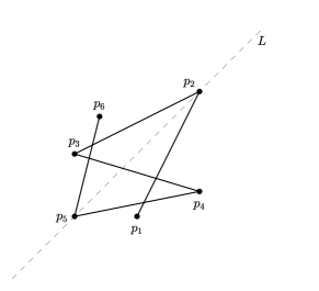
(a)

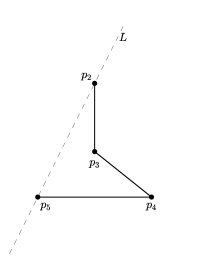
(b)

Figure 2:

Finally, suppose that $\textup{Conv}(S)$ is a quadrangle, but $[p_{2},p_{3}]$ and $[p_{4},p_{5}]$ do not cross. Since $p_{3}$ and $p_{4}$ are on the same side of $L$, $[p_{2},p_{4}]$ crosses $[p_{3},p_{5}]$. Let $q$ be the crossing point of these intervals. Without loss of generality, assume $\delta(p_{3},q)\geq\delta(p_{4},q)$. Then

$$1<\delta(p_{4},p_{5})\leq\delta(p_{4},q)+\delta(q,p_{5})\leq\delta(p_{3},q)+\delta(q,p_{5})=\delta(p_{3},p_{5})\leq 1,$$

a contradiction. This finishes the proof of the lemma. ∎

3.2 Edge-asteroid triples

A set of three edges in a graph is called an edge-asteroid triple if for each pair of the edges, there is a path containing both of the edges that avoids the neighbourhoods of the end-vertices of the third edge.

Lemma 4.

Let $G=(U,W,E)_{c}$ be a co-bipartite UDG. Then $\overline{G}$ contains no edge-asteroid triples.

Proof.

Let $f$ be a representation of the unit disk graph $G$, and for $v\in V(G)$ let $p_{v}=f(v)$. Suppose to the contrary that $\overline{G}$ contains an edge-asteroid triple $\{e_{1},e_{2},e_{3}\}\subset E$. Denote by $u_{i}$ and $w_{i}$ the end-vertices of $e_{i}$, where $u_{i}\in U$, $w_{i}\in W$, $i\in\{1,2,3\}$. For distinct $i,j,k\in\{1,2,3\}$, let $P_{i}$ be a path in $\overline{G}$ that avoids the neighbourhood of $u_{i}$ and the neighbourhood $w_{i}$, and whose terminal edges are $e_{j}$ and $e_{k}$. By Lemma 2 the interval corresponding to an edge of $P_{i}$ crosses $[p_{u_{i}},p_{w_{i}}]$. Since $\overline{G}$ is bipartite, this implies that the images of the vertices in $V(P_{i})\cap U$ lie on one side of $L_{i}=L(p_{u_{i}},p_{w_{i}})$ and the images of the vertices in $V(P_{i})\cap W$ lie on the other side of $L_{i}$. In particular, $p_{u_{j}}$ and $p_{u_{k}}$ lie on one side of $L_{i}$ and $p_{w_{j}}$ and $p_{w_{k}}$ lie on the other side.

On the other hand, since, by Lemma 2, the intervals corresponding to $e_{1},e_{2},e_{3}$ pairwise cross, there exists $i\in\{1,2,3\}$ such that $p_{u_{j}}$ and $p_{w_{k}}$ are on the same side of $L_{i}$. Indeed, if, say, $p_{u_{1}}$ and $p_{u_{2}}$ lie on the same side of $L_{3}$ and $p_{w_{1}}$ and $p_{w_{2}}$ lie on the other side, then necessarily either $L_{1}$ has $p_{u_{2}}$ and $p_{w_{3}}$ on one of its sides or $L_{2}$ has $p_{u_{1}}$ and $p_{w_{3}}$ on one of its sides (see Figure 3(a)). This contradiction establishes the lemma.

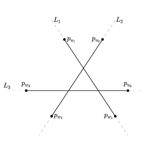
(a)

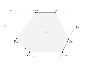
(b)

Figure 3:

∎

Lemma 5.

Let $G=(U,W,E)$ be a bipartite graph. If co-bipartite graph $G^{*}=(U,W,E)_{c}$ is UDG, then $G$ contains no edge-asteroid triples.

Proof.

Let $f$ be a representation of unit disk graph $G^{*}$, and for $v\in V(G^{*})$ let $p_{v}=f(v)$. Suppose to the contrary that $G$ contains an edge-asteroid triple $\{e_{1},e_{2},e_{3}\}\in E$. Denote by $u_{i}$ and $w_{i}$ the end-vertices of $e_{i}$, where $u_{i}\in U$, $w_{i}\in W$, $i\in\{1,2,3\}$. For distinct $i,j,k\in\{1,2,3\}$, let $P_{i}$ be a path in $G$ that avoids the neighbourhoods of $u_{i}$ and $w_{i}$, and whose terminal edges are $e_{j}$ and $e_{k}$. Corollary 1 implies that for every edge $vu$ of $P_{i}$ both $p_{v}$ and $p_{u}$ lie on the same side of $L_{i}=L(p_{u_{i}},p_{w_{i}})$. Therefore all the images of the vertices of $P_{i}$ lie on the same side of $L_{i}$. In particular, $p_{u_{j}},p_{w_{j}},p_{u_{k}}$ and $p_{w_{k}}$ lie on the same side of $L_{i}$. The latter fact means that $p_{u_{1}},p_{w_{1}},p_{u_{2}},p_{w_{2}},p_{u_{3}},p_{w_{3}}$ are extreme points of $C=\textup{Conv}(p_{u_{1}},p_{w_{1}},p_{u_{2}},p_{w_{2}},p_{u_{3}},p_{w_{3}})$ and for every $i\in\{1,2,3\}$ $p_{u_{i}}$ and $p_{w_{i}}$ are adjacent extreme points of the convex hull (see Figure 3(b)).

Now we’ll show that $p_{u_{i}}$ and $p_{w_{j}}$ for $j\neq i$ cannot be adjacent extreme points of the convex hull. Indeed, assume for contradiction, $p_{u_{i}}$ is adjacent to $p_{w_{j}}$ for $j\neq i$. Then, as we proved above, $p_{w_{i}},p_{u_{i}},p_{w_{j}},p_{u_{j}}$ must be a sequence of consecutive extreme points in the convex hull. However, $\{w_{i},u_{i},w_{j},u_{j}\}$ forms a $C_{4}$ in $G^{*}$ and by Lemma 1, $[p_{w_{i}},p_{u_{j}}]$ must be crossing $[p_{w_{j}},p_{u_{i}}]$, a contradiction. Hence, we deduce, that $p_{u_{i}}$ is adjacent to $p_{w_{j}}$ if and only if $i=j$.

Now assume, without loss of generality, that $p_{w_{1}}$ is adjacent to $p_{w_{2}}$ in $C$. This gives us a sequence of extremal points in the convex hull $p_{u_{1}},p_{w_{1}},p_{w_{2}},p_{u_{2}}$. But then $p_{w_{3}}$ is adjacent to either $p_{u_{1}}$ or to $p_{u_{2}}$ in $C$ (see Figure 3(b)), a contradiction.

∎

4 Minimal forbidden induced subgraphs

Theorem 6.

For every integer $k\geq 1$, $\overline{K_{2}+C_{2k+1}}$ is a minimal non-UDG.

Proof.

Let $G=(V,E)$ be a graph isomorphic to $K_{2}+C_{2k+1}$, where $V=\{u,w,c_{1},\ldots,c_{2k+1}\}$ and $E=\{c_{i}c_{j}:|i-j|=1\}\cup\{uw,c_{1}c_{2k+1}\}$. Suppose to the contrary $\overline{G}$ is a UDG and let $f$ be a representation of $\overline{G}$, and let $p_{v}$ denotes $f(v)$ for $v\in V$. By Lemma 2 every linear interval corresponding to an edge of the cycle $C_{2k+1}$ crosses $[p_{u},p_{w}]$. That means that the vertices of the cycle are partitioned into two parts, according to the side of line $L(p_{u},p_{w})$ the image of a vertex belongs to. Moreover, there are no edges between vertices in the same part. This leads to the contradictory conclusion that $C_{2k+1}$ is a bipartite graph.

To prove the minimality of the graphs it is sufficient to show that $\overline{K_{1}+C_{2k+1}}$ is a UDG for any natural $k$. Indeed, notice that by removing a vertex from $\overline{K_{2}+C_{2k+1}}$ we get a graph which is either $\overline{K_{1}+C_{2k+1}}$ or $\overline{K_{2}+P_{2k}}$. The latter one is, in turn, an induced subgraph of $\overline{K_{1}+C_{2k+5}}$. To show that $\overline{K_{1}+C_{2k+1}}$ is a UDG, put $2k+1$ points $p_{0},p_{1},\ldots,p_{2k}$ equally spaced on the circle of radius $r$, i.e. in polar coordinates these points can be written as $(r,0)_{p},(r,\frac{2\pi}{2k+1})_{p},(r,2\frac{2\pi}{2k+1})_{p},\ldots,(r,2k\frac{2\pi}{2k+1})_{p}$. We also add one point $p_{c}$ at the center (0,0). Choose the radius $r$ of the circle such that the distance between $p_{0}$ and $p_{k}$, and between $p_{0}$ and $p_{k+1}$ is greater than 1, and the distances between $p_{0}$ and the other points is at most 1. It is easy to see that the UDG represented by these points is $\overline{K_{1}+C_{2k+1}}$. See Figure 4 for an example of the representation of $\overline{K_{1}+C_{7}}$.

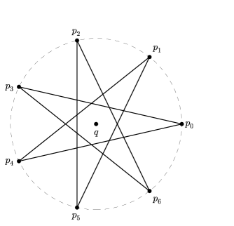
Figure 4: The UDG-representation of $\overline{K_{1}+C_{7}}$

∎

Corollary 2.

For every integer $k\geq 1$, $\overline{P_{k}}$ is UDG.

Theorem 7.

For every integer $k\geq 4$, $\overline{C_{2k}}$ is a minimal non-UDG.

Proof.

Note that by removing a vertex from $\overline{C_{2k}}$ we get $\overline{P_{2k-1}}$, which is UDG by Corollary 2. Therefore it remains to show that $\overline{C_{2k}}$ is not UDG. For $k\geq 5$ the desired result immediately follows from Lemma 4 and the fact that $C_{2k}$ contains an edge-asteroid triple. To prove the result for $k=4$, consider $G=(V,E)$ with $V=\{v_{1},\ldots,v_{8}\}$ and $E=\{(v_{1},v_{8})\}\cup\{(v_{i},v_{j}):|i-j|=1\}$, and let $f$ be a representation of $\overline{G}$, and let $p_{v}$ denotes $f(v)$, as before. By Lemma 2 the linear interval corresponding to an edge of $G$, different from $v_{1}v_{2}$, $v_{1}v_{8}$ and $v_{2}v_{3}$, crosses $[p_{v_{1}},p_{v_{2}}]$. This leads to the conclusion that $p_{v_{3}}$ and $p_{v_{8}}$ are on different sides of $L(p_{v_{1}},p_{v_{2}})$. Therefore $[p_{v_{1}},p_{v_{8}}]$ and $[p_{v_{2}},p_{v_{3}}]$ do not cross, which contradicts Lemma 3. ∎

Theorem 8.

For every integer $k\geq 4$, $C_{2k}^{*}$ is a minimal non-UDG.

Proof.

For $k\geq 5$ the theorem immediately follows from Lemma 5 and the fact that $C_{2k}$ contains an edge-asteroid triple. Notice that $C_{8}^{*}=\overline{C_{8}}$ and hence the conclusion follows from Theorem 7. We remark that one can also prove that $C_{8}^{*}$ is not a unit disk graph by similar means as in Theorem 7 by proving a *-analog of Lemma 3.

To prove the minimality of $C_{2k}^{*}$ it is sufficient to show that $P_{s}^{*}$ is UDG for every natural $s$. Such a representation could be seen in the Figure 8(c) with a description in Theorem 15. ∎

Using Lemmas 4 and 5 one can find more forbidden (not necessarily minimal) induced subgraphs for the class of unit disk graphs. For example, $\overline{S_{3,3,3}}$, $\overline{F_{1}}$, $\overline{F_{2}}$, $\overline{F_{3}}$, $S_{3,3,3}^{*}$, $F_{1}^{*}$, $F_{2}^{*}$ and $F_{3}^{*}$ are forbidden, since each of the graphs $S_{3,3,3}$, $F_{1}$, $F_{2}$ and $F_{3}$ (see Figure 5) contains an edge-asteroid triple. Also, $\overline{F_{4}}$ and $F_{4}^{*}$ are forbidden, as they coincide with $F_{1}^{*}$ and $\overline{F_{1}}$, respectively. The results of the next section imply that all the mentioned forbidden graphs are in fact minimal.

Figure 5: Bipartite graphs $S_{3,3,3}$, $F_{1}$, $F_{2}$ and $F_{3}$ contain an edge-asteroid triple. Graph $F_{4}$ is the bipartite complementation of $F_{1}$.

5 Structure of some subclasses of co-bipartite unit disk graphs

For easier reference, let $C_{6}^{+3c}$ denotes $F_{4}$ which reads “cycle on 6 vertices plus 3 consecutive (pendant) vertices”, $C_{6}^{+3nc}$ denotes $F_{2}$ which reads “cycle on 6 vertices plus 3 non-consecutive (pendant) vertices” and let $C_{6}^{+2l2}$ denotes $F_{3}$ which reads “cycle on 6 vertices plus 2 (consecutive pendant) paths of length 2”. It follows from the previous section that for every co-bipartite unit disk graph $G=(U,W,E)_{c}$, both $G^{*}$ and $\overline{G}$ lie in the class $Free(S_{3,3,3},C_{3},C_{5},C_{6}^{+3c},C_{6}^{+3nc},C_{6}^{+2l2},C_{7},C_{8},\ldots),$ i.e. the class of bipartite graphs which do not contain $S_{3,3,3},C_{6}^{+3c},C_{6}^{+3nc},C_{6}^{+2l2}$ and $C_{k}$ for $k\geq 8$ as induced subgraphs. Thus, obtaining the structure of the graphs in this class and showing which of them give rise to co-bipartite UDGs, would give complete characterization of the class of co-bipartite UDGs. As a step to the desired characterization of co-bipartite UDGs we additionally forbid $C_{4}$ and get structural characterization of graphs in the resulting class

$$\mathcal{X}=Free(S_{3,3,3},C_{3},C_{4},C_{5},C_{6}^{+3c},C_{6}^{+3nc},C_{6}^{+2l2},C_{7},C_{8},\ldots).$$

Further, we show that for every graph $G=(U,W,E)\in\mathcal{X}$ both $G^{*}$ and $\overline{G}$ are UDGs. In other words we obtain both structural and forbidden induced subgraph characterizations for the following two classes of co-bipartite UDGs:

• – the class of $C_{4}^{*}$-free co-bipartite UDGs, i.e. co-bipartite UDGs $G=(U,W,E)_{c}$ such that $G^{*}=(U,W,E)$ do not contain $C_{4}$;

• – the class of $2K_{2}$-free co-bipartite UDGs.

In Section $5.1$ we describe the structure of the graphs in the class $\mathcal{X}$. By the results of the previous section it follows that $\mathcal{Y}\subseteq\mathcal{X}^{*}$ and $\mathcal{Z}\subseteq\overline{\mathcal{X}}$, where $\mathcal{X}^{*}=\{G^{*}:G=(U,W,E)\in\mathcal{X}\}$ and $\overline{\mathcal{X}}=\{\overline{G}:G\in\mathcal{X}\}$. In Section 5.2 we use the structure of graphs in $\mathcal{X}$ to obtain a UDG-representation of every graph in $\mathcal{X}^{*}$. This implies that $\mathcal{Y}=\mathcal{X}^{*}$, and gives both structural and induced forbidden subgraph characterization for the class $\mathcal{Y}$. In Section 5.3 we show that a UDG-representation of $G^{*}$ can be transformed to a UDG-representation of $\overline{G}$, provided that the former representation satisfies certain conditions. Finally, in section 5.4, we use this transformation to deduce UDG-representation for every graph in $\overline{\mathcal{X}}$, which implies that $\mathcal{Z}=\overline{\mathcal{X}}$. As before this gives both structural and forbidden subgraph characterization for the graphs in $\mathcal{Z}$.

5.1 Structure of graphs in $\mathcal{X}$

Notice that the only cycle which is allowed in the class $\mathcal{X}$ is a $C_{6}$, which we call a hexagon. It follows that a graph $G\in\mathcal{X}$ which do not contain a hexagon is a forest without $S_{3,3,3}$. It is not hard to convince oneself that every connected component of a $S_{3,3,3}$-free forest contains a path such that all other vertices are within distance 2 from the vertices of the path. Such graphs consist of caterpillar-like connected components which are known in the literature as lobsters. Gluing vertices of a lobster are the endpoints of a shortest path whose second neighbourhood dominates the graph. See Figure 7(b) for an example of lobster with highlighted gluing vertices. Now we turn to the general case, where $G\in\mathcal{X}$ is allowed to contain a hexagon.

Let $H$ be a hexagon. We say that vertices of a set $S\subseteq V(H)$ of hexagon $H$ are consecutive, if $H[S]$ is connected. Any two vertices of $H$ which are distance 3 away from each other we call a diagonal of $H$. Two hexagons $H_{1}$ and $H_{2}$ are disjoint if $S=V(H_{1})\cap V(H_{2})=\emptyset$, otherwise we say that they share the set $S$. If $|S|=2$ and the two vertices in $S$ are adjacent, we say that the hexagons share an edge.

Lemma 9.

If two hexagons $H_{1}$ and $H_{2}$ of $G\in\mathcal{X}$ are not disjoint then one of the following holds:

• They share exactly one vertex.

• They share an edge.

• They share two vertices that form a diagonal in each of the hexagons.

• They share 4 consecutive vertices, i.e. the intersection of two hexagons is a $P_{4}$.

Further, $E(G[V(H_{1})\cup V(H_{2})])=E(G[V(H_{1})])\cup E(G[V(H_{2})])$.

Proof.

It can be easily checked that in all the other cases a cycle of forbidden length 3, 4, 5, 7 or 8 would arise. ∎

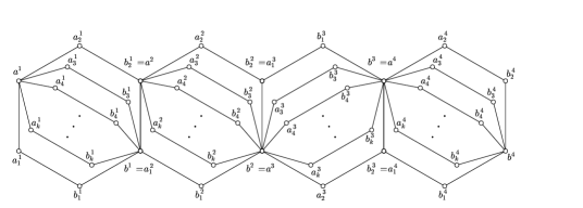
(b) The graph $H(k,1,k,-1,k,-1,k)$

Figure 6: The graphs $C_{6,k}$ and $H(k,1,k,-1,k,-1,k)$

For $k\geq 2$ let us define the graph $C_{6,k}$ to be a graph with $V(C_{6,k})=\{a,b,a_{j},b_{j}:1\leq j\leq k\}$ and $E(C_{6,k})=\{aa_{j},a_{j}b_{j},b_{j}b:1\leq j\leq k\}$ (see Figure 6(a)). In particular, $C_{6,2}$ is isomorphic to $C_{6}$. A connected graph is 2-connected if there is no vertex whose removal disconnects the graph. A maximal 2-connected subgraph of a graph is called 2-connected component of this graph.

Lemma 10.

Let $G\in\mathcal{X}$ be a 2-connected graph with no two hexagons sharing an edge. Then the graph $G$ is isomorphic to $C_{6,k}$ for some $k$.

Proof.

First we will show that there are no two hexagons sharing one vertex. Suppose, for contradiction, there are two hexagons $H_{1}$ and $H_{2}$ with one vertex in common, say $V(H_{1})\cap V(H_{2})=\{v\}$ for some $v\in V(G)$. By Lemma 9, apart from the 12 edges forming two cycles of length 6, there are no other edges in $G[V(H_{1})\cup V(H_{2})]$. Further, one can observe that any vertex $w\in V(G)$ outside the hexagons is adjacent to at most one vertex in $V(H_{1})\cup V(H_{2})$. Indeed, if it has at least two neighbours in $H_{1}$ or at least two neighbours in $H_{2}$ then a cycle of length at most 5 arises. Also, if $w$ is adjacent to one vertex in $H_{1}\setminus v$ and to one vertex in $H_{2}\setminus v$, then either $w$ creates a cycle of length not equal to 6 or $w$ is adjacent to a neighbour of $v$ in one of $H_{1}$ and $H_{2}$, and to the vertex which is diagonally opposite to $v$ in the other hexagon, in which case we have two hexagons sharing an edge, hence again a contradiction. Now, as the graph is 2-connected, there is a path from $V(H_{1})\setminus\{v\}$ to $V(H_{2})\setminus\{v\}$. We pick a path $p=h_{1}v_{1}v_{2}\ldots v_{k}h_{2}$ of minimal length, where $h_{1}\in V(H_{1})\setminus\{v\}$, $h_{2}\in V(H_{2})\setminus\{v\}$, $v_{1},v_{2}\ldots,v_{k}\notin V(H_{1})\cup V(H_{2})$, and $k\geq 2$. Then, $v_{i}$ has at most one neighbour in $V(H_{1})\cup V(H_{2})$ with the neighbour of $v_{1}$ being $h_{1}$, neighbour of $v_{k}$ being $h_{2}$, and $v_{2},v_{3},\ldots,v_{k-1}$ can only be adjacent to $v$ by minimality of the path. Also, by minimality, the path $p$ does not have chords, i.e. edges connecting two non-consecutive vertices of $p$. Now, if $v_{i}$ is adjacent to $v$ for some $i$, then either a cycle of length not equal to 6 arises or there are two hexagons sharing the edge $vv_{i}$. Otherwise, $p$ together with the shortest path between $h_{1}$ and $h_{2}$ in $V(H_{1})\cup V(H_{2})$ either induce a cycle of length more than 6, or one of $h_{1}$ or $h_{2}$ is a neighbour of $v$ in which case we have two hexagons sharing an edge ($vh_{1}$ or $vh_{2}$). The contradiction shows that there are no two hexagons sharing a vertex.

Now, as $G$ is 2-connected it contains a cycle of length 6. Let us consider the maximal subgraph $G^{\prime}$ isomorphic to $C_{6,k}$ containing this cycle. We will show that $G$ coincides with $G^{\prime}$. Suppose not, then there is another hexagon $C$ sharing some vertices with some of the hexagons of $G^{\prime}$. If $C$ shares 4 consecutive vertices with some hexagon, then it must share at least one vertex with each of the hexagons of $G^{\prime}$, which is possible only if $V(C)\cup V(G^{\prime})$ induces $C_{6,k+1}$ in $G$. But this contradicts maximality of $G^{\prime}$. Otherwise, if $C$ shares a diagonal with some of the hexagons of $G^{\prime}$, then it either shares a diagonal with all hexagons or it shares one vertex with some hexagon. The latter case is impossible by the previous paragraph, and the former case proves that $V(C)\cup V(G^{\prime})$ induces $C_{6,k+2}$ contradicting the maximality of $G^{\prime}$. Thus, we deduce that $G$ is isomorphic to $C_{6,k}$. ∎

We say that an edge $xy$ of a graph $G$ is a cutset if $G\setminus\{x,y\}$ has more connected components than $G$.

Lemma 11.

If $G\in\mathcal{X}$ has two hexagons $H_{1}$ and $H_{2}$ sharing an edge, then the edge is a cutset.

Proof.

Let two hexagons share an edge, i.e. $V(H_{1})\cap V(H_{2})=\{v_{1},v_{2}\}$ with $v_{1}v_{2}\in E(G)$. Notice that each vertex in $V(G)\setminus(V(H_{1})\cup V(H_{2}))$ has at most 1 neighbour in $V(H_{1})\cup V(H_{2})$. Indeed, if a vertex has two neighbours in one of the hexagons, then a cycle of length less than 6 arises. If vertex is adjacent to a vertex $h_{1}$ in $H_{1}\setminus\{v_{1},v_{2}\}$ and a vertex $h_{2}$ in $H_{2}\setminus\{v_{1},v_{2}\}$, then the longer path from $h_{1}$ to $h_{2}$ in $G[V(H_{1})\cup V(H_{2})]\setminus\{v_{1}\}$ or in $G[V(H_{1})\cup V(H_{2})]\setminus\{v_{2}\}$ together with $v$ would make a chordless cycle of length more than 6.

Now suppose to the contrary that $G\setminus\{v_{1},v_{2}\}$ is connected. Then, there is a path between $V(H_{1})\setminus\{v_{1},v_{2}\}$ and $V(H_{2})\setminus\{v_{1},v_{2}\}$. Let $p=h_{1}w_{1}w_{2}\ldots w_{k}h_{2}$ be such a path of minimal length, where $h_{1}\in V(H_{1})\setminus\{v_{1},v_{2}\}$ and $h_{2}\in V(H_{2})\setminus\{v_{1},v_{2}\}$. The above discussion implies that $k\geq 2$. Moreover, by minimality of $p$, none of the vertices $w_{1},\ldots,w_{k}$ belongs to $V(H_{1})\cup V(H_{2})$; for $i=2,\ldots,k-1$, if $w_{i}$ has a neighbour in the hexagons, then this neighbour is either $v_{1}$ or $v_{2}$; and the path $p$ does not have chords. Now, let us denote the vertices of $H_{1}$ by $v_{1},v_{2},\ldots,v_{6}$ and vertices of $H_{2}$ by $v_{1},v_{2},v^{\prime}_{3},v^{\prime}_{4},v^{\prime}_{5},v^{\prime}_{6}$ with the edges $\{v_{1}v_{2},v_{2}v_{3},v_{3}v_{4},v_{4}v_{5},v_{5}v_{6},v_{6}v_{1},v_{2}v^{\prime}_{3},v^{\prime}_{3}v^{\prime}_{4},v^{\prime}_{4}v^{\prime}_{5},v^{\prime}_{5}v^{\prime}_{6},v^{\prime}_{6}v_{1}\}$. Then, note that $h_{1}\notin\{v_{3},v_{6}\}$ as otherwise $V(H_{1})\cup\{w_{1},v^{\prime}_{3},v^{\prime}_{6}\}$ induce a $C_{6}^{+3c}$. Similarly, $h_{2}\notin\{v_{3}^{\prime},v_{6}^{\prime}\}$. So without loss of generality we can assume $h_{1}=v_{4}$ and $h_{2}\in\{v^{\prime}_{4},v^{\prime}_{5}\}$. Then the paths connecting $h_{1}$ and $h_{2}$ in $G[V(H_{1})\cup V(H_{2})]\setminus\{v_{1}\}$ and in $G[V(H_{1})\cup V(H_{2})]\setminus\{v_{2}\}$ both have at least 5 vertices. Each of these paths together with the path $p$ form a cycle of length more than 6, and hence each of the cycles has a chord. Let $v_{1}w_{i}$ be a chord in one of the cycles, and $v_{2}w_{j}$ be a chord in the other cycle, such that $i$ and $j$ are smallest possible. Then both $v_{1}v_{6}v_{5}v_{4}w_{1}w_{2}\ldots w_{i}$ and $v_{2}v_{3}v_{4}w_{1}w_{2}\ldots w_{j}$ are chordless cycles. Since every chordless cycle in $G$ is a hexagon, we conclude that $i=2$ and $j=3$. But then $v_{1}v_{2}w_{2}w_{3}$ induce a $C_{4}$. This contradiction finishes the proof. ∎

Let $n\in\mathbb{N}$, and $k_{i}\in\mathbb{N},k_{i}\geq 2$ for every $i=1,\ldots,n$, and $d_{1},\ldots,d_{n-1}\in\{1,-1\}$. Let $C^{i}_{6,k_{i}}$ be a graph isomorphic to $C_{6,k_{i}}$ with $V(C^{i}_{6,k_{i}})=\{a^{i},b^{i},a^{i}_{j},b^{i}_{j}:1\leq j\leq k_{i}\}$ and $E(C^{i}_{6,k_{i}})=\{a^{i}a^{i}_{j},a^{i}_{j}b^{i}_{j},b^{i}_{j}b^{i}:1\leq j\leq k_{i}\}$. A hexagonal strip $H(k_{1},d_{1},k_{2},d_{2},\ldots,k_{n-1},d_{n-1},k_{n})$ is the graph obtained by gluing together $C^{1}_{6,k_{1}},\ldots,C^{n}_{6,k_{n}}$ in such a way that the edge $b^{i}_{2}b^{i}$ is glued to $a^{i+1}a^{i+1}_{1}$ and the direction is described by $d_{i}$:

• if $d_{i}=1$, then $b^{i}_{2}$ is identified with $a^{i+1}$ and $b^{i}$ is identified with $a^{i+1}_{1}$;

• if $d_{i}=-1$, then $b^{i}_{2}$ is identified with $a^{i+1}_{1}$ and $b^{i}$ is identified with $a^{i+1}$.

(a) The graph $C_{6,k}$

Lemma 12.

Let $G$ be a 2-connected graph in $\mathcal{X}$. Then $G$ is isomorphic to $H(k_{1},d_{1},\ldots,k_{n-1},d_{n-1},k_{n})$, for some $n\in\mathbb{N}$, and $k_{i}\in\mathbb{N},k_{i}\geq 2,d_{i}\in\{1,-1\}$, $i=1,\ldots,n$.

Proof.

If two hexagons intersect at an edge then we call such an edge shared. We prove the statement by induction on the number of shared edges. If there are no shared edges, then the conclusion follows from Lemma 10. So suppose there is a shared edge $v_{1}v_{2}$. By the Lemma 11 we know that such an edge is a cutset. Let $C^{\prime}_{1},C^{\prime}_{2},\ldots,C^{\prime}_{k}$ be the components of $G\setminus\{v_{1},v_{2}\}$, and let $C_{i}=G[V(C_{i}^{\prime})\cup\{v_{1},v_{2}\}]$. It is easy to see that each of $C_{1},C_{2},\ldots,C_{k}$ is 2-connected and has less shared edges than $G$. Hence, by induction, each of this graphs is a hexagonal strip. Further, we conclude that $k=2$ and $C_{1}$ and $C_{2}$ are properly glued along $v_{1}v_{2}$ to form a hexagonal strip, because otherwise an induced copy of forbidden $C^{+2l2}$ would arise.

∎

Lemma 13.

Let $G$ be a graph in $\mathcal{X}$ and $H$ be a 2-connected component of $G$. Then $H$ is isomorphic to some hexagonal strip $H(k_{1},d_{1},k_{2},d_{2},\ldots,k_{n-1},d_{n-1},k_{n})$ and vertices $a^{i},b^{i},a^{i}_{1},b^{i}_{2}$ can only be additionally adjacent to some pendant vertices of $G$, with exception of one of $\{a^{1},a^{1}_{1}\}$ and $\{b^{n},b^{n}_{2}\}$. Further, all the other vertices of $G$ do not have any more neighbours in $G\setminus V(H)$.

Proof.

The structure of the $H$ follows from Lemma 12, so we only need to argue about the adjacencies between the vertices in $V(G)\backslash V(H)$ and the vertices in $V(H)$. Consider a connected component $C$ of $G\setminus V(H)$. As $H$ is maximal 2-connected subgraph, the vertices of $C$ can only be adjacent to at most one vertex of $H$. If $C$ has some vertices adjacent to $v\in V(H)$, we will refer to $C$ as a $v$-component. Since $G$ is $C_{3}$-free, we have that every $v$-component of size at least 2, must have two vertices $u,w$ such that $uw,wv\in E(G)$, $u$ is non-adjacent to any vertex of $H$, and $w$ is non-adjacent to any vertex of $H$ other than $v$.

Let us first consider a $v$-component for $v\in\{a^{i},b^{i},a^{i}_{1},b^{i}_{2}:1\leq i\leq n\}\backslash\{a^{1},a^{1}_{1},b^{n},b^{n}_{2}\}$. Suppose the component has size at least 2, hence, by the above argument, the $v$-component has two vertices $u,w\in V(G)\backslash V(H)$ such that $uw,wv\in E(G)$. But then $u,w$ and the two hexagons of $H$, which share an edge containing $v$, form a subgraph containing an induced $C_{6}^{+2l2}$. We conclude that any $v\in\{a^{i},b^{i},a^{i}_{1},b^{i}_{2}:1\leq i\leq n\}\backslash\{a^{1},a^{1}_{1},b^{n},b^{n}_{2}\}$ is adjacent to pendant vertices of $G$ only.

Now, consider a vertex $b^{i}_{k}$ for any $i\neq n$ and $k\neq 2$. Suppose to the contrary, that there is a vertex $w\in V(G)\backslash V(H)$ which is adjacent to $b^{i}_{k}$. Then, $w,b^{i}_{k},a_{2}^{i},a^{i}$ together with $a^{i+1},a^{i+1}_{1},a^{i+1}_{2},b^{i+1}$, $b^{i+1}_{1},b^{i+1}_{2}$ induce a $C^{+2l2}_{6}$. Hence, vertices $b^{i}_{k}$ for any $i\neq n$ and $k\neq 2$, have no neighbours outside $H$. Similarly, one can deduce that $a^{i}_{k}$ has no neighbours for any $i\neq 1$, $k\neq 1$.

We are left to argue about adjacencies of the vertices $a^{1},a^{1}_{i}$ and $b^{n},b^{n}_{i}$. Consider the case when $n>1$. Notice that if $a^{1}_{i}$ and $a^{1}_{j}$ each have a neighbour outside $H$, for some $i\neq j$, then taking the two neighbours together with hexagon $G[a^{1},a^{1}_{i},a^{1}_{j},b^{1}_{i},b^{1}_{j},b_{1}]$, and together with a neighbour of $b^{1}$ either $b^{2}_{1}$ or $a^{2}_{2}$ (depending on wether $a_{1}^{2}$ or $a_{2}$ gets identified with $b^{1}$, respectively), we get an induced $C_{6}^{+3nc}$. This contradiction proves that only one of $a^{1}_{i}$ may have a neighbour outside $H$. Moreover, $a^{1}_{2}$ does not have a neighbour outside $H$, as otherwise an induced $C_{6}^{+3c}$ would arise. Therefore, without loss of generality we can assume that if $a^{1}_{i}$ has a neighbour outside $H$, then $i=1$. It is clear that if there is an $a^{1}$-component and an $a^{1}_{1}$-component which both have sizes at least 2, then we have an induced $C_{6}^{+2l2}$. The analogous arguments holds for $b^{n},b^{n}_{i}$. This finishes the proof for $n>1$. The case $n=1$ can be shown to hold by similar analysis.

∎

Let $G$ be a graph consisting of a hexagonal strip $H(k_{1},d_{1},k_{2},d_{2},\ldots,k_{n-1},d_{n-1},k_{n})$ together with some pendant vertices attached to $a^{i},b^{i},a^{i}_{1},b^{i}_{2}$ and with some radius 2 trees attached to a vertex $a\in\{a^{1},a^{1}_{1}\}$ and a vertex $b\in\{b^{n},b^{n}_{2}\}$. Then we call $G$ a hexagonal caterpillar with gluing vertices $a$ and $b$. Further let $H_{1},H_{2},\ldots,H_{k}$ be a set of vertex disjoint hexagonal caterpillars or lobsters, with $a_{i}$ and $b_{i}$ being gluing vertices of $H_{i}$, for $i=1,\ldots,k$. Then the generalized hexagonal caterpillar $(H_{1},b_{1},a_{2},H_{2},b_{2},a_{3},H_{3},\ldots,b_{k-1},a_{k},H_{k})$ is the graph obtained from $H_{1},H_{2},\ldots,H_{k}$ by identifying pairs of vertices $b_{i}$ and $a_{i+1}$ for every $i=1,\ldots,k-1$.

This description gives us a universal structure for the graphs in $\mathcal{X}$. One can deduce this by noting that any graph in $\mathcal{X}$ should consist of 2-connected components provided by Lemma 13 and lobsters glued together, and that the generalized hexagonal caterpillars described above are the most general graphs we can obtain with this gluing without forming $S_{3,3,3}$. We state this as the main result of this section.

Theorem 14.

Generalized hexagonal caterpillars are universal graphs for the class $\mathcal{X}$, that is each such graph belongs to $\mathcal{X}$ and every graph $G\in\mathcal{X}$ is an induced subgraph of some generalized hexagonal caterpillar.

In further sections we will use the structural characterization of graphs in $\mathcal{X}$ to show that for every $G\in\mathcal{X}$ both $G^{*}$ and $\overline{G}$ are UDGs. First, by Theorem 14 it is enough to prove the result only for generalized hexagonal caterpillars. Further, without loss of generality we can restrict our consideration to those graphs in $\mathcal{X}$ in which no vertex is adjacent to more than one pendant vertex. Indeed, assume a graph $G\in\mathcal{X}$ has a vertex with two pendant neighbours $a$ and $b$. Then $a$ and $b$ belong to the same part in $G$, and therefore to the same part in both $G^{*}$ and $\overline{G}$, in particular $a$ and $b$ are adjacent in these graphs. Moreover, in each of the graphs $N(a)\setminus\{b\}=N(b)\setminus\{a\}$. This implies that if we have a UDG-representation $f$ for $H\setminus\{b\}$, where $H$ is one of $G^{*}$ and $\overline{G}$, then an extension $f^{\prime}$ of $f$ to $V(H)$ with $f^{\prime}(b)=f(a)$ is the UDG-representation for $H$. Therefore, from now on when we refer to a graph in $\mathcal{X}$ we mean a generalized hexagonal caterpillar which is constructed from hexagonal caterpillars or lobsters whose vertices have at most one pendant neighbour (see Figure 7).

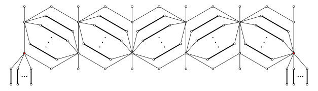
(a) Hexagonal caterpillar with gluing vertices (filled vertices)

(b) Lobsters with gluing vertices (filled vertices)

Figure 7:

5.2 $C_{4}^{*}$-free co-bipartite unit disk graphs

In this section we show that for a graph $G\in\mathcal{X}$ the graph $G^{*}$ is UDG. We do this in two steps. First, we represent basic graphs in $\mathcal{X}^{*}$ and then show how representation of a general graph in $\mathcal{X}^{*}$ can be obtained from a representation of a basic graph. To explain this formally we introduce some definitions.

Let $G$ be a bipartite or co-bipartite graph with parts $U$ and $W$, and let $uw$ be an edge of $G$ with $u\in U$ and $w\in W$. An edge $u^{\prime}w^{\prime}$ of $G$ with $u^{\prime}\in U$ and $w^{\prime}\in W$ is a twin of $uw$ if $N_{W}(u)\triangle N_{W}(u^{\prime})=\{w,w^{\prime}\}$ and $N_{U}(w)\triangle N_{U}(w^{\prime})=\{u,u^{\prime}\}$, where $P\triangle Q$ is the symmetric difference of sets $P$ and $Q$. In this case we also say that the vertex $u^{\prime}$ is a twin of the vertex $u$ and the vertex $w^{\prime}$ is a twin of the vertex $w$. Notice that the relation of being twins is symmetric and transitive. The graph $G$ is basic if it does not contain twin edges. The operation of duplication of the edge $uw$ is to add one or more new edges to $G$ each of which is a twin of $uw$. Note that $uw$ and $u^{\prime}w^{\prime}$ are twins in $G$ if and only if they are twins in $G^{*}$. Each of the thick edges in Figures 7(a) and 7(b) is called parallel edge of hexagonal caterpillar or lobster, respectively. Let $H$ be a generalized hexagonal caterpillar obtained from $H_{1},\ldots,H_{k}$, then an edge of $H$ is called parallel, if it is parallel edge of one of the graphs $H_{1},\ldots,H_{k}$. Similarly, an edge of $H^{*}$ is parallel, if it is parallel edge in $H$. It follows from the results of Section 5.1 that a generalized hexagonal caterpillar is either basic or can be obtained from a basic one by duplicating some of its parallel edges. In Section 5.2.1 we show how to represent graphs in $\mathcal{X}^{*}$ corresponding to basic generalized hexagonal caterpillars, and in Section 5.2.2 we extend this representation to the case of arbitrary generalized hexagonal caterpillars.

5.2.1 Representation of basic graphs

Theorem 15.

Let $G$ be a basic lobster in $\mathcal{X}$. Then $G^{*}$ is UDG.

Proof.

We will show how to obtain UDG-representation $f$ of $G^{*}$ for the lobster $G$ with the vertex set $V(G)=\{g_{i},b_{i},r_{i}:1\leq i\leq n\}$ and edge set $E(G)=\{g_{i}g_{i+1}:1\leq i\leq n-1\}\cup\{g_{i}b_{i},b_{i}r_{i}:1\leq i\leq n\}$. We will refer to the vertices $\mathcal{G}=\{g_{i}:1\leq i\leq n\}$, $\mathcal{B}=\{b_{i}:1\leq i\leq n\}$ and $\mathcal{R}=\{r_{i}:1\leq i\leq n\}$ and to their images in the plane as to green, blue and red, respectively (see Figure 8, for the visualization of the proof). Let us denote the parts of bipartition of $G$ by $C_{1}=\{b_{i},g_{j},r_{k}:1\leq i,j,k\leq n,i$ – odd$,j,k$ – even$\}$ and $C_{2}=\{b_{i},g_{j},r_{k}:1\leq i,j,k\leq n,i$ – even$,j,k$ – odd$\}$. Finally, denote by $\mathcal{G}_{1},\mathcal{B}_{1},\mathcal{R}_{1}$ and $\mathcal{G}_{2},\mathcal{B}_{2},\mathcal{R}_{2}$, the green, blue and red vertices belonging to parts $C_{1}$ and $C_{2}$, respectively.

To put the points on the plane, we first fix some $\mu\in\left(0,\frac{1}{n}\right)$ and draw parallel lines $L_{1},L_{2},L_{3},L_{4}$ such that $L_{2}$ and $L_{3}$ are between $L_{1}$ and $L_{4}$ and $\delta(L_{1},L_{4})=1$, $\delta(L_{2},L_{3})=\sqrt[\ ]{1-\mu^{2}}$, $\delta(L_{1},L_{2})=\delta(L_{3},L_{4})=(1-\sqrt[\ ]{1-\mu^{2}})/2$. Then we draw $k$ lines $\{M_{i}:1\leq i\leq n\}$ perpendicular to line $L_{1}$ and evenly spaced with distance $\mu$ between consecutive ones, i.e. $\delta(M_{1},M_{i})=(i-1)\mu$ for all $1\leq i\leq n$ and all $M_{i}$’s are on one side of $M_{1}$. The intersections between $M_{i}$’s an $L_{j}$’s define the points of our UDG-representation of $G^{*}$ as follows:

• if $i$ is odd, then $f(b_{i})=M_{i}\cap L_{1}$, $f(r_{i})=M_{i}\cap L_{4}$, $f(g_{i})=M_{i}\cap L_{3}$;

• if $i$ is even, then $f(b_{i})=M_{i}\cap L_{4}$, $f(r_{i})=M_{i}\cap L_{1}$, $f(g_{i})=M_{i}\cap L_{2}$.

It is not hard to see that $f(C_{1})\subseteq L_{1}\cup L_{2}$ and $f(C_{2})\subseteq L_{3}\cup L_{4}$. The diameter of $f(C_{1})$ is bounded by $\sqrt[\ ]{\delta(L_{1},L_{2})^{2}+\delta(M_{1},M_{n})^{2}}$. As $\delta(L_{1},L_{2})=\frac{1-\sqrt[\ ]{1-\mu^{2}}}{2}\leq\frac{1-(1-\mu^{2})}{2}=\frac{\mu^{2}}{2}$ and $\delta(M_{1},M_{n})=(n-1)\mu$, we deduce that the diameter of $f(C_{1})$ is at most $n\mu$. By symmetry, the diameter of $f(C_{2})$ is also bounded by $n\mu$. Thus, as $\mu\leq 1/n$, the diameter of each of $f(C_{1})$ and $f(C_{2})$ is at most 1, which correspond to cliques $C_{1}$ and $C_{2}$ in $G^{*}$. It remains to show that $u\in C_{1}$ and $v\in C_{2}$ are adjacent in $G^{*}$ if and only if the distance between the corresponding points $f(u)$ and $f(v)$ is at most 1. Since this is mostly technical task, we moved the confirming calculations to Appendix A. ∎

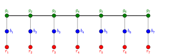
(a) Basic lobster $G$ of length 7

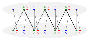
(b) The graph $G^{*}$. Vertices in a gray area form a clique

(c) The UDG-representation of $G^{*}$

Figure 8:

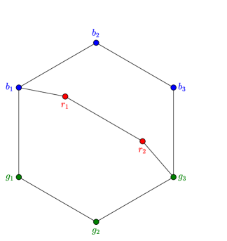
(a) The graph $C_{6,1}$

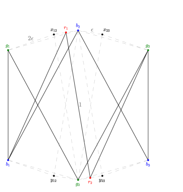
(b) The UDG-representation of $C_{6,1}^{*}$

Figure 9:

Theorem 16.

Let $G$ be a basic graph in $\mathcal{X}$. Then $G^{*}$ is UDG.

Proof.

We will abuse the notation and instead of calling the image of a vertex $v$ by $f(v)$, we will refer to it simply by $v$. Thus, when talking about adjacencies, $v$ will be considered as a vertex of the graph $G^{*}$, and when talking about distances, or some other geometric properties, $v$ will mean the point $f(v)$. We denote $n=|V(G)|$ and we fix a positive parameter $\epsilon<\min\left\{\frac{1}{15n},\frac{1}{128}\right\}$.

Single hexagon. We start by representing graph $G^{*}$ when $G$ is isomorphic to $C_{6,1}$ (see Figure 9(a)). Let $V(G)=\{g_{1},g_{2},g_{3},b_{1},b_{2},b_{3},r_{1},r_{2}\}$ and $E(G)=\{g_{1}g_{2},g_{2}g_{3},g_{3}b_{3},b_{3}b_{2},b_{2}b_{1},b_{1}g_{1},b_{1}r_{1},r_{1}r_{2},r_{2}g_{3}\}$. To construct a UDG-representation $f$ of $G^{*}$, first, we place 6 points $\{x_{12},b_{2},x_{23},y_{12},g_{2},y_{23}\}$ in the plane forming two rectangles as follows (see Figure 9(b)):

• $\{x_{12},b_{2},y_{23},g_{2}\}$ forms a $1\times\epsilon$ rectangle, where $\delta(x_{12},g_{2})=\delta(b_{2},y_{23})=1$, $\delta(x_{12},b_{2})=\delta(g_{2},y_{23})=\epsilon$ and $[x_{12},g_{2}]$ is perpendicular to $[g_{2},y_{23}]$.

• $\{b_{2},x_{23},g_{2},y_{12}\}$ forms a $1\times\epsilon$ rectangle, where $\delta(b_{2},y_{12})=\delta(x_{23},g_{2})=1$, $\delta(b_{2},x_{23})=\delta(y_{12},g_{2})=\epsilon$ and $[b_{2},x_{23}]$ is perpendicular to $[x_{23},g_{2}]$, and $x_{23}\neq x_{12}$.

Further, we place points $\{g_{1},g_{3},b_{1},b_{3}\}$ as shown in Figure 9(b) such that:

• $\delta(g_{1},g_{2})=\delta(g_{2},g_{3})=\delta(b_{1},b_{2})=\delta(b_{2},b_{3})=1$.

• $\delta(g_{1},x_{12})=\delta(g_{3},x_{23})=\delta(b_{1},y_{12})=\delta(b_{3},y_{23})=2\epsilon$.

Finally, we place the points $\{r_{1},r_{2}\}$ as follows:

• $r_{1}$ in the middle of the segment $[x_{12},b_{2}]$, $r_{2}$ in the middle of the segment $[g_{2},y_{23}]$.

We argue that this is indeed a UDG-representation of $G^{*}$. First of all, observe that the two parts of bipartition of $G$ are $C_{1}=\{g_{1},g_{3},b_{2},r_{1}\}$ and $C_{2}=\{b_{1},b_{3},g_{2},r_{2}\}$. By triangle inequalities, one may obtain that the distances between the points in $f(C_{1})$ (resp. $f(C_{2})$) are at most $6\epsilon<1$. Hence we only need to deal with distances between $f(C_{1})$ and $f(C_{2})$. Note that $\{b_{2},r_{1},g_{2},r_{2}\}$ belongs to the rectangle $\textup{Conv}(x_{12},b_{2},y_{23},g_{2})$ and then it is easy to see that $\delta(r_{1},r_{2})=1$ and the other distances $\delta(r_{1},g_{2}),\delta(r_{2},b_{2}),\delta(b_{2},g_{2})$ between these points are at least $\sqrt[\ ]{1+(\epsilon/2)^{2}}\geq 1+\epsilon^{2}/16$. The rest of the pairs of vertices in the different parts $C_{1}$ and $C_{2}$ include a “corner” vertex – $g_{1},g_{3},b_{1}$ or $b_{3}$, and by symmetry, it is enough to show

• Claim 1. $\delta(g_{1},y)\leq 1$ for all $y\in[b_{1},y_{12}]\cup[y_{12},g_{2}]$; and

• Claim 2. $\delta(g_{1},y)>1$ for all $y\in(g_{2},y_{23}]\cup[y_{23},b_{3}]$.

One can see that Claim 1 holds, by extending the segment $[g_{1},b_{1}]$ to $[g_{1},b]$ such that $\triangle g_{1}bg_{2}$ is a right-angled triangle with diagonal $[g_{1},g_{2}]$ of length $1$, and $[g_{1},b]$ being perpendicular to $[b,g_{2}]$. Then, noticing that $y_{12}$ and $b_{1}$ lie inside this triangle, we conclude, that all the points of $[b_{1},y_{12}]\cup[y_{12},g_{2}]$ lie inside this triangle and have distances at most 1 to any vertex of the triangle (in particular to $g_{1}$). We note that one can be more precise and by estimating the projections calculate that the distance between $g_{1}$ and $y_{12}$ is at most $\sqrt[\ ]{1-(\epsilon/2)^{2}}\leq 1-\epsilon^{2}/8$ and the distance between $g_{1}$ and the midpoint of $[y_{12},g_{2}]$ is at most $\sqrt[\ ]{1-(\epsilon/4)^{2}}\leq 1-\epsilon^{2}/32$. Also, one can calculate that the distance between $g_{1}$ and $b_{1}$ is between $1-10\epsilon^{2}$ and $1-9\epsilon^{2}$ (this estimate holds for $\epsilon<1/5$).

Regarding Claim 2, one should first observe that $\textup{Conv}(g_{1},g_{2},b_{2},x_{12})$ is a quadrilateral, i.e. $x_{12}$ indeed lies above the line $g_{1}b_{2}$ in the Figure 9 (and by symmetry $y_{23}$ lies below $g_{2}b_{3}$). This follows from the fact that $\triangle g_{1}x_{12}g_{2}$ is an isosceles triangle with $\angle g_{2}g_{1}x_{12}=\angle g_{1}x_{12}g_{2}=\alpha<90$. Thus $\angle g_{1}x_{12}b_{2}=\alpha+90<180$. From this we deduce that $\angle b_{2}g_{1}g_{2}<\alpha<90$ and hence $\angle g_{1}g_{2}b_{3}>90$. The latter inequality implies that any point on $(g_{2},b_{3}]$ has distance greater than $\delta(g_{1},g_{2})=1$ and hence we are done. Indeed, it is not hard to evaluate using the Pythagorean theorem, that $\delta(g_{1},y_{23})\geq\sqrt[\ ]{1+\epsilon^{2}}\geq 1+\epsilon^{2}/4$ and $\delta(g_{1},r_{2})\geq\sqrt[\ ]{1+(\epsilon/2)^{2}}\geq{1+\epsilon^{2}/16}$.

Two hexagons sharing an edge. Now we proceed to showing how to represent $G^{*}$, where $G$ consists of two $C_{6,1}$ sharing an edge, and two additional pending vertices $a_{3}$ and $h_{3}$ (see Figure 10(a)). The corresponding representation is illustrated in Figure 10(b). Points $a_{3},h_{3}$ are placed in such a way that:

• $a_{3},h_{3}\in L(b_{3},g_{3})$ and $\delta(a_{3},b_{3})=1$, $\delta(g_{3},h_{3})=1$, as shown in the picture.

It is easy to see that distance from $a_{3}$ to every point in the opposite part except $b_{3}$ is larger than 1, or indeed larger than $\sqrt[\ ]{1+(2\epsilon)^{2}}$. By symmetry, the same holds for points $h_{3}$ and $g_{3}$. The distances involving points $g_{3}$ and $b_{3}$ are as needed for UDG-representation, because these points belong to both hexagons. For the rest distances, it is enough to show the following

• Claim 3. For any $x\in[x_{34},b_{4}]\cup[b_{4},x_{45}]\cup[x_{45},g_{5}]$ and any $y\in[y_{23},g_{2}]\cup[g_{2},y_{12}]\cup[y_{12},b_{1}]$, $\delta(x,y)>1$.

For any $y\in[b_{1},y_{12}]\cup[y_{12},g_{2})$ and any $x\in[g_{3},x_{34}]\cup[x_{34},b_{4}]\cup[b_{4},x_{45}]\cup[x_{45},y_{5}]$ we have that $\delta(x,y)\geq\delta(g_{3},y)>1$ by argument in Claim 2. Thus, to prove Claim 3, we can restrict ourselves to $y\in[g_{2},y_{23}]$. By symmetry, we can also restrict to $x\in[x_{34},b_{4}]$, for which it is enough to prove that $\delta(y_{23},x_{34})>1$. One can easily convince oneself that $\delta(x_{12},x_{23})<\delta(x_{23},x_{34})$, hence $\delta(y_{23},x_{34})=\sqrt[\ ]{\delta(y_{23},x_{23})^{2}+\delta(x_{23},x_{34})^{2}}>\sqrt[\ ]{\delta(y_{23},x_{23})^{2}+\delta(x_{12},x_{23})^{2}}=\delta(x_{12},y_{23})=\sqrt[\ ]{1+\epsilon^{2}}$. Therefore Claim 3 holds and we are done with joining two hexagons by an edge. Moreover, it is not hard to see that the arguments in Claims 1-3 extend to any collection of edge-adjacent hexagons, i.e. to a basic hexagonal caterpillar with attached pendant vertices.

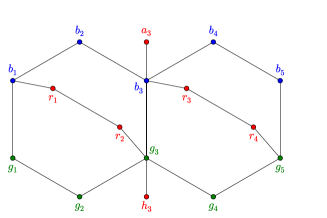
(a) Two hexagons joined along an edge

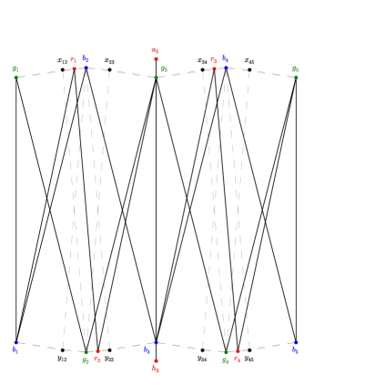
(b) The UDG-representation of two hexagons joined along an edge

Figure 10:

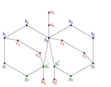
(a) Two hexagons sharing a vertex

(b) The UDG-representation of two hexagons sharing a vertex

Figure 11:

Two hexagons sharing a vertex. Now we will show how to represent $G^{*}$, where $G$ consists of two $C_{6,1}$ sharing a vertex (see Figure 11(a)). The representation is obtained from the above representation for two hexagons sharing an edge, but we replace the vertex $g_{3}$ by two vertices $g_{3}^{\prime}$ and $g_{3}^{\prime\prime}$ (see Figure 11(b)) such that:

• $g_{3}^{\prime}$ is the midpoint of $[g_{3},x_{23}]$ and $g_{3}^{\prime\prime}$ is the midpoint of $[g_{3},x_{34}]$.

To prove that the points $g_{3}^{\prime}$ and $g_{3}^{\prime\prime}$ have proper distances in the two adjacent hexagons, and in a chain of hexagons sharing a vertex or an edge, we will show the following

• Claim 4. Denote the midpoints of $[b_{1},y_{12}]$, $[y_{12},g_{2}]$, $[y_{34},g_{4}]$, $[y_{45},b_{5}]$ by $b_{1}^{\prime\prime},R_{2},R_{4},b_{5}^{\prime}$, respectively. Then, for $x\in\{b_{1},b_{1}^{\prime\prime},R_{2},R_{4},g_{4},r_{4},b_{5}^{\prime},b_{5}\}$ we have $\delta(g_{3}^{\prime},x)>1$ and for $x\in\{g_{2},r_{2},b_{3}\}$ we have $\delta(g_{3}^{\prime},x)<1$.

The proof of Claim 4 is given in Appendix B.1. We notice that the proof for distances from $g_{3}^{\prime}$ to $R_{2},R_{4},b_{1}^{\prime\prime}$ and $b_{5}^{\prime}$, ensures that $g_{3}^{\prime}$ has correct adjacencies with respect to all possible choices of direction of diagonals in hexagons and with possibility of having further hexagons adjacent at a single vertex $g_{1}$ or $g_{5}$. Finally, we place the points $\{h_{3}^{\prime},h_{3}^{\prime\prime},a_{3},a_{4}\}$ in the plane as follows:

• $a_{3}$ is the midpoint of $[g_{3}^{\prime},g_{3}^{\prime\prime}]$ and $h_{3}^{\prime},a_{4}$, $h_{3}^{\prime\prime}$ are distance 1 below the points $g_{3}^{\prime},a_{3}$ and $g_{3}^{\prime\prime}$, respectively.

It is clear that each of $h_{3}^{\prime},a_{4},h_{3}^{\prime\prime}$ is distance more than 1 away from all the vertices in the upper part except $g_{3}^{\prime},a_{3},g_{3}^{\prime\prime}$, respectively. Hence we only need to verify the distances involving $a_{3}$. Observe that for all $y\in[b_{1},y_{12}]\cup[y_{12},g_{2}]$ we have $\delta(a_{3},y)>\delta(g_{3},y)\geq 1$. Also $\delta(a_{3},b_{3})<\delta(g_{3}^{\prime},b_{3})<1$. Hence, it is enough to show that $\delta(a_{3},r_{2})>1$. The proof of the latter fact can be found in Appendix B.2.

Connecting a chain of hexagons with a lobster. To finish the proof, we will show how a chain of hexagons can be attached to a lobster. An example is pictured in Figure 12. To attach hexagon to a lobster at vertex $g_{7}$, we use the representation of hexagon obtained for joining hexagons at one vertex, i.e. we use point $b_{7}^{\prime}$ with an attached pending vertex and point $g_{7}$ with a leg of size 2 attached exactly as in construction of hexagon joined to another hexagon at a vertex. This ensures that the first leg of lobster is attached correctly. Then we use the construction of lobster obtained in Theorem 15. In Theorem 15, the lobster was uniquelly determined by a parameter $\mu$. The distance between two inner lines $L_{2}$ and $L_{3}$ was $\sqrt[\ ]{1-\mu^{2}}$. Here, we choose $\mu$ to be such that this distance is equal to $\delta(g_{1},b_{1})$. For the record, as we noted before, $1-10\epsilon^{2}\leq\delta(g_{1},b_{1})\leq 1-9\epsilon^{2}$ implies that $(1-10\epsilon^{2})^{2}\leq 1-\mu^{2}\leq(1-9\epsilon^{2})^{2}$. Expanding, one can estimate that $1-25\epsilon^{2}\leq(1-10\epsilon^{2})^{2}$ and for $\epsilon<1/9$, we can obtain the estimate $(1-9\epsilon^{2})^{2}\leq 1-16\epsilon^{2}$. Hence it follows that $4\epsilon\leq\mu\leq 5\epsilon$, which is roughly represented as the spacing between the lobster legs in the Figure 12(b). It easily follows that the inner vertices of lobster are more than 1 away from any inner (not belonging to lobster) vertices of any hexagon. This completes the proof that for any basic graph $G\in\mathcal{X}$, $G^{*}$ is representable as a UDG.

∎

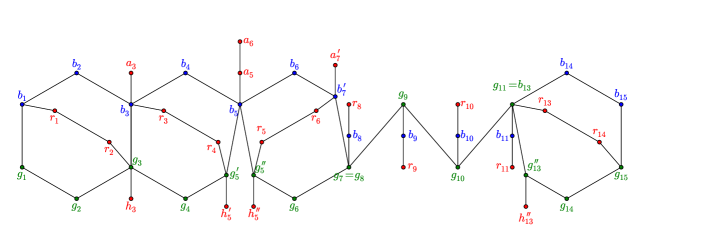
(a) Hexagonal caterpillar

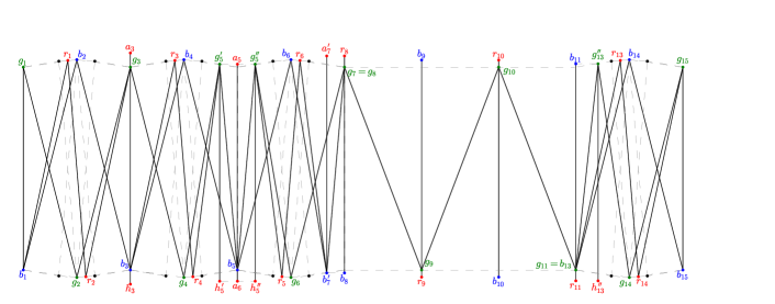
(b) The UDG-representation of hexagonal caterpillar

Figure 12:

In the following theorem we prove several properties of representation of basic graphs that are important for representation of general graphs.

Theorem 17 (Properties of basic graph representation).

Let $G=(U,W,E)_{c}$ be a basic $C_{4}^{*}$-free co-bipartite UDG with $n=|V(G)|$. Then for every positive $\epsilon<\min\{\frac{1}{15n},\frac{1}{128}\}$ there exist $\Delta,q,r$ with $0<\Delta<\frac{1}{3}$, $0<q\leq r<6$, and a UDG-representation $f:V(G)\rightarrow\mathbb{R}^{2}$ of $G$ with the following properties:

1. $f(U)\subseteq D_{1}$ and $f(W)\subseteq D_{2}$, where $D_{1}=[0,\Delta]\times[\Lambda,\Lambda]$, $D_{2}=[0,\Delta]\times[1-\Lambda,1+\Lambda]$ with $\Lambda=r\epsilon^{2}$;

2. For any vertices $a\in U$ and $b\in W$ either $\delta_{f}(a,b)=1$ or $|\delta_{f}(a,b)-1|\geq q\epsilon^{2}$;

3. For every parallel edge $ab$ of $G$, $\delta_{f}(a,b)=1$. Moreover, $\delta_{f}(a,c)\neq 1$ and $\delta_{f}(c,b)\neq 1$ for any vertex $c\in V(G)$ different form $a$ and $b$.

Proof.

Let $f$ be a representation obtained in Theorem 16. To the assumption that $\epsilon<\frac{1}{128}$ made in the theorem, we also add $\epsilon<\frac{1}{15n}$ to ensure that the representation lies in the strip of length $\Delta<\frac{1}{3}$. One can obtain such estimate by noting that the distance in $x$-coordinate between two consecutive points is less than $5\epsilon$, hence, the $n$ points will fit in the strip of length $5n\epsilon<\frac{1}{3}$. Observe that the shortest distance in $y$-coordinate between two points from different parts is obtained by $\delta_{f}(g_{1},b_{1})$ and it is at least $1-10\epsilon^{2}$. Also observe that every point has at least 1 neighbour in the other part, i.e. distance at most 1 from some point in another part. From these two observations, we can conclude that all the points lie in two strips of width $10\epsilon^{2}$ which are distance $1-10\epsilon^{2}$ away from each other. Hence, it follows that $r=5$ satisfies the conditions. From the proof of the theorem it is also not hard to see that we can take $q=\frac{1}{64}$. Finally, notice that every parallel edge satisfies property (3), so we are done. ∎

5.2.2 Representation of general graphs

Let $G=(U,W,E)_{c}$ be an arbitrary graph from $\mathcal{X}^{*}$ and let $H$ be a basic graph in $\mathcal{X}^{*}$ such that $G$ is obtained from $H$ by duplicating some of its parallel edges. In this section we show how to extend a representation of $H$ described in the previous section to a representation of $G$. We also prove that the resulting representation possesses certain properties, that will be important in Section 5.3.

Let $e_{i}=a_{i}b_{i},i=1,\ldots,s$ be parallel edges of $H$ that have twins in $G$. For $i=1,\ldots,s$ let $e_{i}^{j}=a_{i}^{j}b_{i}^{j},j=1,\ldots,k_{i}$, be twin edges of $e_{i}$ in $G$, and let $k=k_{1}+\cdots+k_{s}$. We say that vertices in $V(G)\setminus V(H)$ are new vertices. For convenience we let $a_{i}^{0}=a_{i}$ and $b_{i}^{0}=b_{i}$. Let $h$ be a representation of $H$ with chosen positive $\epsilon<\min\left\{\frac{1}{15|V(H)|},\frac{1}{128}\right\}$ and parameters $\Delta$, $q$ and $r$ guaranteed by Theorem 17.

First we define an extension $g:V(G)\rightarrow\mathbb{R}^{2}$ of $h$ and then show that $g$ is a representation of $G$. To define $g$ we choose $t=\frac{q}{64\sqrt[\ ]{r}}>0$ and let $t_{1}=\frac{t}{k}$. Since $g$ is an extension of $h$, it maps all vertices of $H$ to the same points as $h$ does, that is $g(x)=h(x)$ for every $x\in V(H)$. Further, we define mapping of new vertices. Informally, for the edge $e_{i}=a_{i}b_{i}$ we place $a_{i}^{j},b_{i}^{j},j=1,\ldots,k_{i}$ in the plane in such a way that $a_{i},b_{i},a_{i}^{k_{i}},b_{i}^{k_{i}}$ form a “narrow” rectangle with $[a_{i},b_{i}]$ and $[a_{i}^{k_{i}},b_{i}^{k_{i}}]$ being parallel sides, and $[a_{i}^{j},b_{i}^{j}],j=1,\ldots,k_{i}-1$ are segments parallel to $[a_{i},b_{i}]$ and evenly spaced within the rectangle. Formally, for every $i=1,\ldots,s$ and $j=1,\ldots,k_{i}$ we define $g(a_{i}^{j})$ and $g(b_{i}^{j})$ in such a way that:

1. the segment $[g(a_{i}^{j}),g(b_{i}^{j})]$ is parallel to the segment $[g(a_{i}),g(b_{i})]$;

2. $\delta_{g}(a_{i}^{j},b_{i}^{j})=1$;

3. $\delta_{g}(a_{i},a_{i}^{j})=\delta_{g}(b_{i},b_{i}^{j})=j\frac{t}{k}\epsilon=jt_{1}\epsilon$;

4. $\delta_{g}(a_{i}^{j},a_{i}^{j+1})=\delta_{g}(b_{i}^{j},b_{i}^{j+1})=\frac{t}{k}\epsilon=t_{1}\epsilon$ (for $j=0,\ldots,k_{i}-1$);

5. each of the segments $[g(a_{i}),g(a_{i}^{j})]$ and $[g(b_{i}),g(b_{i}^{j})]$ is perpendicular to the segment $[g(a_{i}),g(b_{i})]$;

6. (for definiteness) $g(a_{i}^{j})$ and $g(b_{i}^{j})$ have larger $x$-coordinate than $g(a_{i})$ and $g(b_{i})$, respectively.

To prove that $g$ is a UDG-representation of $G$ we need several auxiliary statements.

Lemma 18.

Suppose $ab$ is a parallel edge. Then the angle $\alpha$ between $[g(a),g(b)]$ and the vertical line, satisfies $\sin(\alpha)\leq 2\sqrt[\ ]{r}\epsilon$.

Proof.

Let $g(a)=(x,y)$, $g(b)=(x^{\prime},y^{\prime})$. As $\delta_{g}(a,b)$=1, we have $\sin(\alpha)=|x-x^{\prime}|$. Notice that since $a$ and $b$ are in different parts, we get $|y-y^{\prime}|\geq 1-2r\epsilon^{2}$. From this it follows that

$$\sin(\alpha)=|x-x^{\prime}|=\sqrt[\ ]{1-|y-y^{\prime}|^{2}}\leq\sqrt[\ ]{1-1+4r\epsilon^{2}}\leq 2\sqrt[\ ]{r}\epsilon.$$

∎

Lemma 19.

Let $a,a^{\prime}\in V(G)$ be twins, and let $g(a)=(x,y)$, $g(a^{\prime})=(x^{\prime},y^{\prime})$. Then $|x-x^{\prime}|\leq t\epsilon$ and $|y-y^{\prime}|\leq 2t\sqrt[\ ]{r}\epsilon^{2}$.

Proof.

Clearly, the first inequality holds because $|x-x^{\prime}|\leq\delta_{g}(a,a^{\prime})\leq t\epsilon$. Now, $|y-y^{\prime}|=\delta_{g}(a,a^{\prime})\sin(\alpha)$ where $\alpha$ is the angle between segment $[a,a^{\prime}]$ and the horizontal line. This angle is equal to the angle of the parallel edge and vertical line, thus, by previous lemma we can deduce that $\sin(\alpha)\leq 2\sqrt[\ ]{r}\epsilon$. Hence,

$$|y-y^{\prime}|=\delta_{g}(a,a^{\prime})\sin(\alpha)\leq 2t\sqrt[\ ]{r}\epsilon^{2}.$$

∎

The following is an important lemma which will be used for proving that the defined map $g$ is indeed a UDG-representation of $G$.

Lemma 20.

Suppose $a,b$ are two vertices in different parts of $G$ with $|\delta_{g}(a,b)-1|\geq q\epsilon^{2}$. Let $a^{\prime}$ be either a twin of $a$ or $a^{\prime}=a$ and let $b^{\prime}$ be either a twin of $b$ or $b^{\prime}=b$. Then $\delta_{g}(a^{\prime},b^{\prime})>1$ iff $\delta_{g}(a,b)>1$ and $|\delta_{g}(a^{\prime},b^{\prime})-1|\geq q\epsilon^{2}/2$.

Proof.

Let $a=(x,y)$, $a^{\prime}=(x^{\prime},y^{\prime})$, $b=(z,u)$, $b^{\prime}=(z^{\prime},u^{\prime})$. To get the bounds of the distance $\delta_{g}(a^{\prime},b^{\prime})$, we will compare projections of $[g(a^{\prime}),g(b^{\prime})]$ and $[g(a),g(b)]$ onto $x$ and $y$ axes and then apply the Pythagorean theorem.

First of all, triangle inequalities can be used to obtain that $|x-z|\leq|x-x^{\prime}|+|x^{\prime}-z^{\prime}|+|z-z^{\prime}|$ and $|x^{\prime}-z^{\prime}|\leq|x^{\prime}-x|+|x-z|+|z-z^{\prime}|$. Further, by Lemma 19, we have $|x-x^{\prime}|\leq t\epsilon$ and $|z-z^{\prime}|\leq t\epsilon$, and hence

$$|x-z|-2t\epsilon\leq|x^{\prime}-z^{\prime}|\leq|x-z|+2t\epsilon.$$ (6)

Similarly, projecting onto $y$-axis, from triangle inequalities we obtain $|y^{\prime}-u^{\prime}|\leq|y^{\prime}-y|+|y-u|+|u-u^{\prime}|$ and $|y-u|\leq|y-y^{\prime}|+|y^{\prime}-u^{\prime}|+|u^{\prime}-u|$. Also from Lemma 19 we know that $|y-y^{\prime}|\leq 2t\sqrt[\ ]{r}\epsilon^{2}$ and $|u-u^{\prime}|\leq 2t\sqrt[\ ]{r}\epsilon^{2}$. This gives us

$$|y-u|-4t\sqrt[\ ]{r}\epsilon^{2}\leq|y^{\prime}-u^{\prime}|\leq|y-u|+4t\sqrt[\ ]{r}\epsilon^{2}.$$ (7)

Now, we split our analysis into two cases.

Case 1. $|x-z|>4\sqrt[\ ]{r}\epsilon$.

Since $|y-u|\geq 1-2r\epsilon^{2}$, we can easily obtain that

$$\delta_{g}(a,b)^{2}=|y-u|^{2}+|x-z|^{2}>(1-2r\epsilon^{2})^{2}+(4\sqrt[\ ]{r}\epsilon)^{2}=1+12r\epsilon^{2}+4r^{2}\epsilon^{4}>1.$$

Hence, in this case our aim is to prove that $\delta_{g}(a^{\prime},b^{\prime})>1$ and $|\delta_{g}(a^{\prime},b^{\prime})-1|\geq q\epsilon^{2}/2$, i.e. we have to prove that $\delta_{g}(a^{\prime},b^{\prime})\geq 1+q\epsilon^{2}/2$. For this, we use the estimates of the projections

$$|x^{\prime}-z^{\prime}|\geq |x-z|-2t\epsilon\geq 4\sqrt[\ ]{r}\epsilon-2t\epsilon;$$

$$|y^{\prime}-u^{\prime}|\geq |y-u|-4t\sqrt[\ ]{r}\epsilon^{2}\geq 1-2r\epsilon^{2}-4t\sqrt[\ ]{r}\epsilon^{2}.$$

As $q\leq r$, we have $t=\frac{q}{64\sqrt[\ ]{r}}\leq\frac{\sqrt[\ ]{r}}{2}$, and placing this upper bound of $t$ into the above inequalities we obtain

$$|x^{\prime}-z^{\prime}|\geq 4\sqrt[\ ]{r}\epsilon-\sqrt[\ ]{r}\epsilon=3\sqrt[\ ]{r}\epsilon;$$

$$|y^{\prime}-u^{\prime}|\geq 1-2r\epsilon^{2}-2r\epsilon^{2}=1-4r\epsilon^{2}.$$

Applying the Pythagorean theorem, we obtain

$$\delta_{g}(a^{\prime},b^{\prime})^{2}\geq(3\sqrt[\ ]{r}\epsilon)^{2}+(1-4r\epsilon^{2})^{2}=9r\epsilon^{2}+1-8r\epsilon^{2}+16r^{2}\epsilon^{4}\geq 1+r\epsilon^{2}+r^{2}\epsilon^{4}/4=(1+r\epsilon^{2}/2)^{2}.$$

Hence, $\delta_{g}(a^{\prime},b^{\prime})\geq 1+r\epsilon^{2}/2$, and as $r\geq q$, we obtain the required inequality $\delta_{g}(a^{\prime},b^{\prime})\geq 1+q\epsilon^{2}/2$.

Case 2. $|x-z|\leq 4\sqrt[\ ]{r}\epsilon$.

First, consider

$$||x^{\prime}-z^{\prime}|^{2}-|x-z|^{2}|=||x^{\prime}-z^{\prime}|-|x-z||\times||x^{\prime}-z^{\prime}|+|x-z||.$$

By (6) we have that the first term $||x^{\prime}-z^{\prime}|-|x-z||$ is upper bounded by $2t\epsilon$, and the second by

$$|x^{\prime}-z^{\prime}|+|x-z|\leq 2|x-z|+2t\epsilon\leq 8\sqrt[\ ]{r}\epsilon+2t\epsilon\leq 10\sqrt[\ ]{r}\epsilon,$$

where the latter inequality follows from the fact that $t=\frac{q}{64\sqrt[\ ]{r}}\leq\frac{r}{64\sqrt[\ ]{r}}\leq\sqrt[\ ]{r}$. This gives us an upper bound

$$||x^{\prime}-z^{\prime}|^{2}-|x-z|^{2}|\leq 2t\epsilon\times 10\sqrt[\ ]{r}\epsilon=20t\sqrt[\ ]{r}\epsilon^{2}.$$ (8)

Similarly, consider

$$||y^{\prime}-u^{\prime}|^{2}-|y-u|^{2}|=||y^{\prime}-u^{\prime}|-|y-u||\times||y^{\prime}-u^{\prime}|+|y-u||.$$

By (7), we have $||y^{\prime}-u^{\prime}|-|y-u||\leq 4t\sqrt[\ ]{r}\epsilon^{2}$ and

$$|y^{\prime}-u^{\prime}|+|y-u|\leq 2|y-u|+4t\sqrt[\ ]{r}\epsilon^{2}\leq 2(1+2r\epsilon^{2})+4t\sqrt[\ ]{r}\epsilon^{2}\leq 3.$$

This gives us an upper bound

$$||y^{\prime}-u^{\prime}|^{2}-|y-u|^{2}|\leq 4t\sqrt[\ ]{r}\epsilon^{2}\times 3\leq 12t\sqrt[\ ]{r}\epsilon^{2}.$$ (9)

Adding (8) and (9), we get

$$|\delta_{g}(a^{\prime},b^{\prime})^{2}-\delta_{g}(a,b)^{2}|\leq 32t\sqrt[\ ]{r}\epsilon^{2}.$$

One can easily check, for example by projecting to $y$-axis, that $\delta_{g}(a,b)+\delta_{g}(a^{\prime},b^{\prime})\geq 1$. Hence,

$$|\delta_{g}(a^{\prime},b^{\prime})-\delta_{g}(a,b)|\leq 32t\sqrt[\ ]{r}\epsilon^{2}/(\delta_{g}(a,b)+\delta_{g}(a^{\prime},b))\leq 32t\sqrt[\ ]{r}\epsilon^{2}.$$

Inserting $t=\frac{q}{64\sqrt[\ ]{r}}$ we have

$$|\delta_{g}(a^{\prime},b^{\prime})-\delta_{g}(a,b)|\leq q\epsilon^{2}/2.$$

As $|\delta_{g}(a,b)-1|\geq q\epsilon^{2}$, it follows that $|\delta_{g}(a^{\prime},b^{\prime})-1|\geq q\epsilon^{2}/2$ and that $\delta_{g}(a^{\prime},b^{\prime})>1$ iff $\delta_{g}(a,b)>1$. This completes the proof of the lemma.

∎

We are now ready to prove the main results of this section.

Theorem 21.

Suppose $h$ is a UDG-representation of the basic graph $H$ which satisfies the conditions outlined in Theorem 17. Let $\epsilon,r,q,\Delta$ be as in Theorem 17. Then $g$ is a UDG-representation of $G=(U,W,E)_{c}$. Moreover, the representation $g$ satisfies the following conditions:

• $g(U)\subseteq D_{1}$, $g(W)\subseteq D_{2}$ where $D_{1}=[0,\Delta^{\prime}]\times[-\Lambda,\Lambda]$, $D_{2}=[0,\Delta^{\prime}]\times[1-\Lambda,1+\Lambda]$ with $\Lambda=r^{\prime}\epsilon^{2}$, $r^{\prime}=2r$, and $\Delta^{\prime}=\Delta+\epsilon$.

• For every $u\in U$, $w\in W$, we have either $\delta_{g}(u,w)=1$ or $|\delta_{g}(u,w)-1|\geq q^{\prime}\epsilon^{2}$ for $q^{\prime}=\frac{q^{2}}{64^{2}r\times 4k^{2}}$.

Proof.

The condition (2) is satisfied for all the vertices of $H$ by Theorem 17. Further, by Lemma 20, the condition is satisfied between any new vertex and a vertex of $H$, or between two new vertices that are twins of vertices in different parallel edges. So we only need to consider pairs of new vertices $a_{i}^{l}$, $b_{i}^{m}$, $l,m\in\{1,2,\ldots,k_{i}\}$ that are twins to two vertices of the same parallel edge $a_{i}b_{i}$. In this case, clearly, the distances that are not equal to $1$ are at least

$$\sqrt[\ ]{1+\left(\frac{t}{k}\epsilon\right)^{2}}\geq 1+\frac{t^{2}}{4k^{2}}\epsilon^{2}=1+\frac{q^{2}}{64^{2}r\times 4k^{2}}\epsilon^{2}.$$

The condition (1) is clearly satisfied for the representation $h$ of $H$, and by Lemma 19, we can get out of the strip horizontally by at most $t\epsilon<\epsilon$ and vertically by at most $4t\sqrt[\ ]{r}\epsilon^{2}<r\epsilon^{2}$. This completes the proof. ∎

As for any basic graph $G\in\mathcal{X}^{*}$ we have a UDG-representation satisfying the conditions of Theorem 17, Theorem 21 shows that every graph in $\mathcal{X}^{*}$ is a UDG. Moreover, the representation has several properties, that allow us to transform these UDG-representations to UDG-representations of the bipartite complements of these graphs, which we will do in the next section. For completeness we state the result for general graphs in $\mathcal{X}^{*}$.

Theorem 22.

Let $G=(U,W,E)_{c}$ be an $n$-vertex graph in $\mathcal{X}^{*}$. Then for every sufficiently small $\Lambda$ there exists $\Delta^{\prime}\in(0,1/3)$, and a UDG-representation $g$ of $G$ possessing the following properties:

• $g(U)\subseteq D_{1}$, $g(W)\subseteq D_{2}$, where $D_{1}=[0,\Delta^{\prime}]\times[-\Lambda,\Lambda]$, $D_{2}=[0,\Delta^{\prime}]\times[1-\Lambda,1+\Lambda]$.

• For every $u\in U$, $w\in W$, we have either $\delta_{g}(u,w)=1$ or $|\delta_{g}(u,w)-1|\geq q^{\prime\prime}\Lambda$, where $q^{\prime\prime}=\frac{1}{64^{4}\times 200n^{2}}$.

Proof.

Let $g$ be a UDG-representation of $G$ with parameters $\epsilon,r^{\prime},q^{\prime},\Delta^{\prime},\Lambda$ guaranteed by Theorem 21. First we can assume that $\Delta^{\prime}\in(0,1/3)$, which is true for every sufficiently small $\epsilon$, since $\Delta^{\prime}=\Delta+\epsilon$ and $\Delta\in(0,1/3)$. Now for arbitrary $u\in U$ and $w\in W$, if $\delta_{g}(u,w)\neq 1$, then $|\delta_{g}(u,w)-1|\geq q^{\prime}\epsilon^{2}$ and from $\Lambda=r^{\prime}\epsilon^{2}$ we derive

$$|\delta_{g}(u,w)-1|\geq\frac{q^{\prime}}{r^{\prime}}\Lambda=\frac{q^{2}}{64^{2}r\times 4k^{2}\times 2r}\Lambda\geq\frac{1}{64^{4}\times 200n^{2}}\Lambda=q^{\prime\prime}\Lambda,$$

where we take $q=\frac{1}{64}$ and $r=5$, which is eligible as shown in the proof of Theorem 17. ∎

5.3 On bipartite self-complementarity of the class of co-bipartite UDGs

Notice that all the forbidden subgraphs (and, more generally, substructures) for co-bipartite unit disk graphs, which were revealed in Sections 3 and 4 are self-complementary in bipartite sense, i.e. if $G$ is a bipartite graph and $G^{*}$ is a forbidden subgraph, then $\overline{G}$ is also a forbidden subgraph. This in turn motivates to explore, whether the class of co-bipartite UDGs is indeed self-complementary in bipartite sense. In this section, we show that if a UDG-representation of a co-bipartite graph $G^{*}$ satisfies certain conditions, then it can be transformed into a UDG-representation of the graph $\overline{G}$. Loosely speaking, the conditions tells us that the parts of $G^{*}$ are mapped into two narrow strips being distance approximately 1 away from each other. In the next section we will apply this result to show that the bipartite complement of a $C_{4}^{*}$-free co-bipartite UDG is also UDG. This will settle the fact that $\mathcal{Z}=\overline{\mathcal{X}}$.

In this section we will often use polar coordinates. Let us recall that a point $(r,\alpha)_{p}$ in polar coordinates is a point $(r\cos(\alpha),r\sin(\alpha))$ in standard Cartesian coordinates. We begin by describing the transformation. For this we fix $0<\Lambda<\frac{1}{12}$ and $0<\Delta<\frac{1}{3}$ and let $D_{1}=[0,\Delta]\times[-\Lambda,\Lambda]\subseteq\mathbb{R}^{2}$, $D_{2}=[0,\Delta]\times[1-\Lambda,1+\Lambda]\subseteq\mathbb{R}^{2}$. Let $D=D_{1}\cup D_{2}$ be the domain where the points of the representation of $G^{*}$ lie. The transformation $\tau:D\rightarrow\mathbb{R}^{2}$ is defined as follows (see Figure 13 for illustration):

$$\text{for all $\alpha\in[0,\Delta]$ and $y\in[-\Lambda,\Lambda]$, define }\begin{cases}\tau(\alpha,y):=\left(\frac{1}{2}+y,-\frac{\pi}{2}+2\alpha\right)_{p}&\\ \tau(\alpha,1+y):=\left(\frac{1}{2}-y,\frac{\pi}{2}+2\alpha\right)_{p}&\end{cases}$$

Notice first that this transformation maps set of points on a horizontal line to a line through $(0,0)$. That is for a fixed $\alpha$ the points $D_{1}(\alpha)=\{(\alpha,y_{1}):y_{1}\in[-\Lambda,\Lambda]\}$ and $D_{2}(\alpha)=\{(\alpha,1+y_{2}):y_{2}\in[-\Lambda,\Lambda]\}$ are mapped to the line

$$L(\alpha)=\left\{\left(y,\frac{\pi}{2}+2\alpha\right)_{p}:y\geq 0\right\}\bigcup\left\{\left(y,-\frac{\pi}{2}+2\alpha\right)_{p}:y>0\right\}.$$

To closer examine what happens on the line, take two points $A=(\alpha,y_{1})\in D_{1}(\alpha)$ and $B=(\alpha,1+y_{2})\in D_{2}(\alpha)$ for some $y_{1},y_{2}\in[-\Lambda,\Lambda]$. Then $\delta(A,B)=1+y_{2}-y_{1}$ and $\delta(\tau(A),\tau(B))=\frac{1}{2}+y_{1}+\frac{1}{2}-y_{2}=1+y_{1}-y_{2}$. Therefore

• if $y_{1}-y_{2}=0$, then $\delta(A,B)=1$ and $\delta(\tau(A),\tau(B))=1$;

• if $y_{1}-y_{2}=a>0$ then $\delta(A,B)=1-a<1$ and $\delta(\tau(A),\tau(B))=1+a>1$;

• if $y_{1}-y_{2}=-a<0$ then $\delta(A,B)=1+a>1$ and $\delta(\tau(A),\tau(B))=1-a<1$.

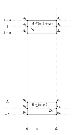
(a)

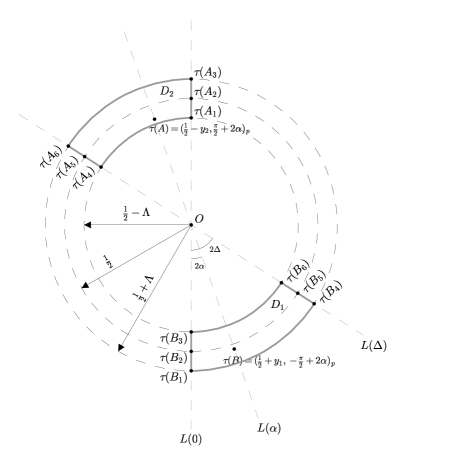
(b)

Figure 13: Transformation $\tau$

Thus, for two points $A\in D_{1}(\alpha)$, $B\in D_{2}(\alpha)$ on the same horizontal line but in different parts, transformation $\tau$ swaps the distances that are less than 1 with the distances that are greater than 1, i.e. $\delta(\tau(A),\tau(B))>1$ iff $\delta(A,B)<1$ and $\delta(\tau(A),\tau(B))<1$ iff $\delta(A,B)>1$. Further, one can easily see that both $\tau(D_{1})$ and $\tau(D_{2})$ have diameter less than 1. Thus, if we have a UDG-representation $f$ of some co-bipartite graph $G^{*}$ which lies on one horizontal line, i.e. $f(G^{*})\subseteq D_{1}(\alpha)\cup D_{2}(\alpha)$ and avoids distances equal to one, then the map $\tau\mathbin{\mathchoice{\vbox{\hbox{$\scriptstyle\circ$}}}{\vbox{\hbox{$\scriptstyle\circ$}}}{\vbox{\hbox{$\scriptscriptstyle\circ$}}}{\vbox{\hbox{$\scriptscriptstyle\circ$}}}}f$ is a UDG-representation of $\overline{G}$.

We would like to extend this argument to the whole set $D_{1}\cup D_{2}$. However, not all the distances, between the points in different parts $D_{1}$ and $D_{2}$, which are less than 1 will be swapped with distances that are greater than 1 by map $\tau$. Nevertheless, in the lemma below we will show that the distances that are smaller than $1-100\Lambda^{2}$ or greater than $1+100\Lambda^{2}$ are mapped to distances greater than 1 or smaller than 1, respectively. Thus, if $G^{*}$ has a UDG-representation $g$ with $g(G^{*})\subseteq D_{1}\cup D_{2}$ such that no distance lies in the interval $[1-100\Lambda^{2},1+100\Lambda^{2}]$, then $\tau\mathbin{\mathchoice{\vbox{\hbox{$\scriptstyle\circ$}}}{\vbox{\hbox{$\scriptstyle\circ$}}}{\vbox{\hbox{$\scriptscriptstyle\circ$}}}{\vbox{\hbox{$\scriptscriptstyle\circ$}}}}g$ is a UDG-representation of $\overline{G}$. Furthermore, it is worth noting that the distances of size 1 can be avoided by appropriate scaling of the initial UDG-representation, as we will see later. Now we are ready to prove the main result of this section.

Lemma 23.

Let $D_{1}$ and $D_{2}$ be as described above. Suppose $G^{*}$ admits a UDG-representation $g$, such that $g(V(G^{*}))\subseteq D_{1}\cup D_{2}$ and for all $x\in D_{1}\cap g(V(G^{*})),y\in D_{2}\cap g(V(G^{*}))$, $\delta(x,y)\notin[1-100\Lambda^{2},1+100\Lambda^{2}]$. Then $\tau\mathbin{\mathchoice{\vbox{\hbox{$\scriptstyle\circ$}}}{\vbox{\hbox{$\scriptstyle\circ$}}}{\vbox{\hbox{$\scriptscriptstyle\circ$}}}{\vbox{\hbox{$\scriptscriptstyle\circ$}}}}g$ is a UDG-representation of $\overline{G}$.

Proof.

We will prove the lemma by showing that for any two points $A=(\alpha,1+a)$, $B=(\beta,b)$, with $\alpha,\beta\in[0,\Delta]$ and $a,b\in[-\Lambda,\Lambda]$ the following statement holds:

• if $\delta(A,B)<1-100\Lambda^{2}$ or $\delta(A,B)>1+100\Lambda^{2}$, then $\delta(\tau(A),\tau(B))>1$ or $\delta(\tau(A),\tau(B))<1$, respectively.

First we observe that it is enough to show the statement ($\star$) for all pairs $A,B$ as above with $\alpha=0$. Indeed, let $\alpha^{\prime}=\min(\alpha,\beta)$ and $\beta^{\prime}=\max(\alpha,\beta)$ and let $A^{\prime}=(\alpha^{\prime},1+a)$, $B^{\prime}=(\beta^{\prime},b)$. It is not hard to see that $\delta(A^{\prime},B^{\prime})=\delta(A,B)$ and $\delta(\tau(A^{\prime}),\tau(B^{\prime}))=\delta(\tau(A),\tau(B))$. Further, let $\beta^{\prime\prime}=\beta^{\prime}-\alpha^{\prime}$ and let $A^{\prime\prime}=(0,1+a)$, $B^{\prime\prime}=(\beta^{\prime\prime},b)$. Again, it is not hard to see that $\delta(A^{\prime},B^{\prime})=\delta(A^{\prime\prime},B^{\prime\prime})$ and $\delta(\tau(A^{\prime}),\tau(B^{\prime}))=\delta(\tau(A^{\prime\prime}),\tau(B^{\prime\prime}))$, because horizontal shifting by distance $\alpha^{\prime\prime}$ and rotating around the origin by angle $2\alpha^{\prime\prime}$ are both isometries of the plane. Thus, the pair $A,B$ satisfies ($\star$) iff the pair $A^{\prime\prime},B^{\prime\prime}$ satisfies ($\star$). Hence from now onwards we will assume $A=(0,1+a),B=(\beta,b)$, with $\beta\in[0,\Delta]$ and $a,b\in[-\Lambda,\Lambda]$.

Consider a special point $S=(\beta,s)$ with $s=s(\beta,a)<1$ such that $\delta(A,S)=1$ (see Figure 14). This point is an intersection of the vertical line going through $(\beta,0)$ and a unit circle centered at $A$ and one can easily calculate that $s=a+1-\sqrt[\ ]{1-\beta^{2}}$. The importance of the point $S$ is that the distance between $A$ and a point $B=(\beta,b)$ is greater or smaller than 1 depending on whether $B$ is below (i.e. $b<s$) or above (i.e. $b>s$) $S$, respectively.

Similarly, consider a special point $Q$ which lies on the ray $R(\beta)=\left\{\left(r,-\frac{\pi}{2}+2\beta\right)_{p}:r\geq 0\right\}\subseteq L(\beta)$ and is distance 1 away from $\tau(A)=\left(0,\frac{1}{2}-a\right)$. Such a point exists and is unique because the unit cycle centered at $\left(0,\frac{1}{2}-a\right)$ contains the origin O - the endpoint of the half-line. We denote the distance $q=q(\beta,a)=\delta(O,Q)-\frac{1}{2}$. The importance of the point $Q$ is that it divides the ray $R(\beta)$ into two segments: the points $\left(\frac{1}{2}+b,-\frac{\pi}{2}+2\beta\right)_{p}$ have distance less or more than 1 from $\tau(A)$ depending on whether $b<q$ or $b>q$, respectively. Let $Q^{\prime}=(\beta,q)$. As $\left(\frac{1}{2}+b,-\frac{\pi}{2}+2\beta\right)_{p}=\tau(\beta,b)$ for any $b\in[-\Lambda,\Lambda]$, we deduce that $\delta(\tau(B),\tau(A))$ is greater or smaller than 1 depending on whether $B$ lies above or below the point $Q^{\prime}$, respectively.

From the above discussion we deduce the following important criterion. If $b>\max\{q(\beta,a),s(\beta,a)\}$, then $\delta(A,B)<1$, and $\delta(\tau(A),\tau(B))>1$. Similarly, if $b<\min\{q(\beta,a),s(\beta,a)\}$, then $\delta(A,B)>1$, and $\delta(\tau(A),\tau(B))<1$. So, in both cases $B=(\beta,b)$ satisfies ($\star$). However, if $b\in[\min\{q,s\},\max\{q,s\}]$, then the distances are not inverted by the map $\tau$, i.e. either $\delta(A,B)$ and $\delta(\tau(A),\tau(B))$ are both smaller or equal to 1 or both greater than 1. In what follows, we will show that in this case $\delta(A,B)\in[1-100\Lambda^{2},1+100\Lambda^{2}]$. In order to do so, we will estimate values of $q$ and $s$ more precisely.

As we observed earlier $s=a+1-\sqrt[\ ]{1-\beta^{2}}$. We can approximate the root part of the equation as follows: $1-\frac{\beta^{2}}{2}-\frac{\beta^{4}}{2}\leq\sqrt[\ ]{1-\beta^{2}}\leq 1-\frac{\beta^{2}}{2}$. Hence,

$$a+\frac{\beta^{2}}{2}\leq s\leq a+\frac{\beta^{2}}{2}+\frac{\beta^{4}}{2}.$$

For finding reasonable bounds of function $q$ the arguments are more involved, and we moved them to Appendix C, where we show

$$a+\frac{\beta^{2}}{2}-\frac{7\beta^{4}}{6}-2a^{2}\beta^{2}\leq q\leq a+\frac{\beta^{2}}{2}+\frac{\beta^{4}}{2}.$$

Having obtained these estimates, we are now ready to say something about non-invertible points, that is the points $B=(\beta,b)\in D_{1}$ such that $\delta(A,B)$ and $\delta(\tau(A),\tau(B))$ are both greater or both smaller than 1. As we observed above, such $B$ must lie between $Q^{\prime}$ and $S$, i.e. must have $b\in[\min\{q,s\},\max\{q,s\}]$. Further we consider two cases with respect to the value of $\beta$.

1. $\beta>\sqrt[\ ]{6\Lambda}$. The obtained bounds on the functions $q$ and $s$ imply that

   $$\min\{q(\beta,a),s(\beta,a)\}\geq a+\frac{\beta^{2}}{2}-\frac{7\beta^{4}}{6}-2a^{2}\beta^{2}\geq-\Lambda+\beta^{2}\left(\frac{1}{2}-\frac{7\beta^{2}}{6}-2\Lambda^{2}\right)$$

   $$\geq -\Lambda+\beta^{2}\left(\frac{1}{2}-\frac{7}{6}\times\frac{1}{9}-\frac{2}{12^{2}}\right)\geq-\Lambda+\frac{\beta^{2}}{3}$$

   $$> -\Lambda+\frac{\left(\sqrt[\ ]{6\Lambda}\right)^{2}}{3}=-\Lambda+2\Lambda=\Lambda.$$

   Hence there is no point in $[\min\{q,s\},\max\{q,s\}]\cap[-\Lambda,\Lambda]$, which means that every point $B\in\beta\times[-\Lambda,\Lambda]$ satisfies ($\star$): $\delta(A,B)>1$ but $\delta(\tau(A),\tau(B))<1$.

2. $\beta\leq\sqrt[\ ]{6\Lambda}$. In this region, we have:

   $$|q(\beta,a)-s(\beta,a)|\leq a+\frac{\beta^{2}}{2}+\frac{\beta^{4}}{2}-\left(a+\frac{\beta^{2}}{2}-\frac{7\beta^{4}}{6}-2a^{2}\beta^{2}\right)$$

   $$= \frac{5\beta^{4}}{3}+2a^{2}\beta^{2}\leq\frac{5\left(\sqrt[\ ]{6\Lambda}\right)^{4}}{3}+\frac{2\Lambda^{2}}{9}$$

   $$= \left(60+\frac{2}{9}\right)\Lambda^{2}\leq 100\Lambda^{2}$$

   If $B$ is non-invertible, then it satisfies $\min\{q,s\}\leq b\leq\max\{q,s\}$ and we have $\delta(B,S)\leq|q-s|\leq 100\Lambda^{2}$. The triangle inequalities $\delta(B,S)+\delta(A,B)\geq\delta(A,S)$ and $\delta(B,S)+\delta(A,S)\geq\delta(A,B)$ imply

   $$\delta(A,S)-\delta(B,S)\leq\delta(A,B)\leq\delta(A,S)+\delta(B,S),$$

   and as $\delta(A,S)=1$, we deduce $1-100\Lambda^{2}\leq\delta(A,B)\leq 1+100\Lambda^{2}$. This finishes the proof that any $A=(0,1+a)\in D_{2}$ and any $B=(\beta,b)\in D_{1}$ satisfies ($\star$) and hence the proof of the lemma.

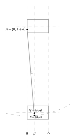
(a)

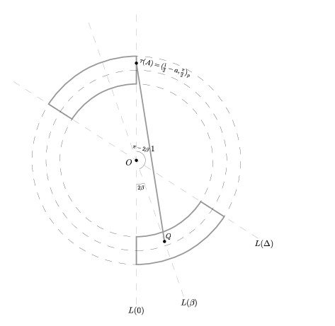
(b)

Figure 14: Special points $S$ and $Q$ (here $a<0$)

∎

5.4 $2K_{2}$-free co-bipartite unit disk graphs

Now we are ready to use the results of the above section to transform the representation of a $C_{4}^{*}$-free co-bipartite unit disk graph into a representation of its bipartite complement, which is a $2K_{2}$-free co-bipartite graph.

Theorem 24.

Let $G=(U,W,E)$ be a graph in $\mathcal{X}$. Then $\overline{G}$ is a UDG.

Proof.

First let us choose some $\Lambda<\frac{q^{\prime\prime}}{1600}$ satisfying the conditions of Theorem 22 with $q^{\prime\prime}$ as in the theorem. By Theorem 22 we know that ${G}^{*}$ has a UDG-representation $g$ such that:

1. $g(U)\subseteq D_{1}$, $g(W)\subseteq D_{2}$, where $D_{1}=[0,\Delta]\times[-\Lambda,\Lambda]$, $D_{2}=[0,\Delta]\times[1-\Lambda,1+\Lambda]$, for some $\Delta\in(0,1/3)$;

2. for any two vertices $u\in U$ and $w\in W$, we have either $\delta_{g}(u,w)=1$ or $|\delta_{g}(u,w)-1|\geq q^{\prime\prime}\Lambda$.

To employ Lemma 23 for transforming the UDG-representation $g$ to a UDG-representation of $\overline{G}$, we must get rid of unit distances. To this end we first apply scaling transformation

$$h:(x,y)\rightarrow\left(\left(1-\frac{q^{\prime\prime}}{2}\Lambda\right)x,\left(1-\frac{q^{\prime\prime}}{2}\Lambda\right)y\right),$$

which scales the whole map by a factor of $1-\frac{q^{\prime\prime}}{2}\Lambda$. One can observe that distance between images of any two vertices in different parts of $G^{*}$ under the map $h\mathbin{\mathchoice{\vbox{\hbox{$\scriptstyle\circ$}}}{\vbox{\hbox{$\scriptstyle\circ$}}}{\vbox{\hbox{$\scriptscriptstyle\circ$}}}{\vbox{\hbox{$\scriptscriptstyle\circ$}}}}g$ is either at most $1-\frac{q^{\prime\prime}\Lambda}{2}$ or at least

$$(1+q^{\prime\prime}\Lambda)\times\left(1-\frac{q^{\prime\prime}}{2}\Lambda\right)=1+\frac{q^{\prime\prime}}{2}\Lambda-\frac{q^{\prime\prime 2}}{2}\Lambda^{2}>1+\frac{q^{\prime\prime}}{2}\Lambda-\frac{q^{\prime\prime}}{4}\Lambda=1+\frac{q^{\prime\prime}}{4}\Lambda,$$

where the latter inequality is valid because $q^{\prime\prime}<1$ and $\Lambda<1/2$. Therefore, for any vertices $u,w$ in different parts of $G^{*}$, we have $|\delta_{h\mathbin{\mathchoice{\vbox{\hbox{$\scriptstyle\circ$}}}{\vbox{\hbox{$\scriptstyle\circ$}}}{\vbox{\hbox{$\scriptscriptstyle\circ$}}}{\vbox{\hbox{$\scriptscriptstyle\circ$}}}}g}(u,w)-1|\geq\frac{q^{\prime\prime}}{4}\Lambda$. Also note that $\delta_{h\mathbin{\mathchoice{\vbox{\hbox{$\scriptstyle\circ$}}}{\vbox{\hbox{$\scriptstyle\circ$}}}{\vbox{\hbox{$\scriptscriptstyle\circ$}}}{\vbox{\hbox{$\scriptscriptstyle\circ$}}}}g}(u,w)>1$ iff $\delta_{g}(u,w)>1$, hence $h\mathbin{\mathchoice{\vbox{\hbox{$\scriptstyle\circ$}}}{\vbox{\hbox{$\scriptstyle\circ$}}}{\vbox{\hbox{$\scriptscriptstyle\circ$}}}{\vbox{\hbox{$\scriptscriptstyle\circ$}}}}g$ is a UDG-representation of $G^{*}$. We must also note that the scaling affected the strips $D_{1}$ and $D_{2}$ as well. Though, it is not hard to check that the images of $D_{1}$ and $D_{2}$ under the map $h\mathbin{\mathchoice{\vbox{\hbox{$\scriptstyle\circ$}}}{\vbox{\hbox{$\scriptstyle\circ$}}}{\vbox{\hbox{$\scriptscriptstyle\circ$}}}{\vbox{\hbox{$\scriptscriptstyle\circ$}}}}g$ fall into the strips $[0,\Delta]\times[-2\Lambda,2\Lambda]$ and $[0,\Delta]\times[1-2\Lambda,1+2\Lambda]$, respectively.

Finally, the choice of $\Lambda$ guarantees that $2\Lambda<\frac{1}{12}$ and $|\delta_{h\mathbin{\mathchoice{\vbox{\hbox{$\scriptstyle\circ$}}}{\vbox{\hbox{$\scriptstyle\circ$}}}{\vbox{\hbox{$\scriptscriptstyle\circ$}}}{\vbox{\hbox{$\scriptscriptstyle\circ$}}}}g}(u,w)-1|\geq\frac{q^{\prime\prime}}{4}\Lambda>100(2\Lambda)^{2}$. Hence Lemma 23 applies to the UDG-representation $h\mathbin{\mathchoice{\vbox{\hbox{$\scriptstyle\circ$}}}{\vbox{\hbox{$\scriptstyle\circ$}}}{\vbox{\hbox{$\scriptscriptstyle\circ$}}}{\vbox{\hbox{$\scriptscriptstyle\circ$}}}}g$ of $G^{*}$ and gives us a transformation map $\tau$, such that $\tau\mathbin{\mathchoice{\vbox{\hbox{$\scriptstyle\circ$}}}{\vbox{\hbox{$\scriptstyle\circ$}}}{\vbox{\hbox{$\scriptscriptstyle\circ$}}}{\vbox{\hbox{$\scriptscriptstyle\circ$}}}}h\mathbin{\mathchoice{\vbox{\hbox{$\scriptstyle\circ$}}}{\vbox{\hbox{$\scriptstyle\circ$}}}{\vbox{\hbox{$\scriptscriptstyle\circ$}}}{\vbox{\hbox{$\scriptscriptstyle\circ$}}}}g$ is a UDG-representation of $\overline{G}$. This finishes the proof of the theorem. ∎

6 Concluding remarks and open problems

In this work we identified infinitely many new minimal forbidden induced subgraphs for the class of unit disk graphs. Using these results we provided structural characterization of some subclasses of co-bipartite UDGs. Obtaining structural characterization of the whole class of co-bipartite UDGs is a challenging research problem. An open problem for which such a characterization may be useful is the problem of implicit representation of UDGs. A hereditary class $\mathcal{G}$ admits an implicit representation if there exists a positive integer $k$ and a polynomial algorithm $A$ such that the vertices of every $n$-vertex graph $G\in\mathcal{G}$ can be assigned labels (binary strings) of length at most $k\log n$ such that given two vertex labels of $G$ algorithm $A$ correctly decides adjacency of the corresponding vertices in $G$ [12]. Notice that a class $\mathcal{G}$ admitting an implicit representation has $2^{O(n\log n)}$ $n$-vertex graphs as only $O(n\log n)$ bits is used for encoding each of these graphs. In [12] Kannan et al. asked whether converse is true, i.e. is it true that every hereditary class having $2^{O(n\log n)}$ $n$-vertex graphs admits an implicit representation? In [17] Spinrad restated this question as a conjecture, which nowadays is known as the implicit graph conjecture. The class of UDGs satisfies the conditions of the conjecture, i.e. it is hereditary and contains $2^{\Theta(n\log n)}$ $n$-vertex graphs (see [17] and [15]). Though, no adjacency labeling scheme for the class is known [17]. A natural approach for such labeling would be to associate with every vertex the coordinates of its image under an UDG-representation in $\mathbb{Q}^{2}$. For this idea to work the integers (numerators and denominators) involved in coordinates of points in the UDG-representation should be bounded by a polynomial of $n$. However, as shown in [14] this can not be guaranteed as there are $n$-vertex UDGs for which every UDG-representation necessarily uses at least one integer of order $2^{2^{\Omega(n)}}$. Therefore some further ideas required for tackling the problem. For example one may try to combine geometrical and structural properties of UDGs maybe together with some additional tools (see e.g. [1]) to attack the problem of implicit representation of UDGs. In particular, from our structural results one can derive an implicit representation for $C_{4}^{*}$-free co-bipartite UDGs and for $2K_{2}$-free co-bipartite UDGs. However, it remains unclear how to get an implicit representation for the whole class of co-bipartite UDGs, and it would be very interesting to see such results.

Interestingly, for every discovered co-bipartite forbidden subgraph and substructure its bipartite complementary counterpart is also forbidden. This suggests that the class of co-bipartite UDGs may be closed under bipartite complementation. This intuition is further supported by the result that the bipartite complement of a $C_{4}^{*}$-free co-bipartite UDG is also (co-bipartite) UDG. These facts lead us to pose the following

Conjecture.

For every co-bipartite UDG its bipartite complement is also co-bipartite UDG.

One of the possible approaches to prove this conjecture is, similarly to the proof of Lemma 23, to show that a representation of a co-bipartite UDG can be transformed into a representation of its bipartite complementation.

Another interesting research direction is to investigate systematically properties of edge asteroid triple free graphs as it was done for asteroidal triple free graphs [6]. Similarly to co-bipartite UDGs edge asteroid triples arose in forbidden subgraph characterizations of several other graph classes such as co-bipartite circular arc graphs [9] and bipartite 2-directional orthogonal ray graphs [16]. However, knowledge about edge asteroid triple free graphs is sporadic, and it would be interesting to study in a consistent manner properties of these graphs, especially, of those graphs which are bipartite.

Appendices

A Addendum to the proof of Theorem 15

Distances between points in $f(C_{1})$ and $f(C_{2})$

We split the arguments into cases where we argue about pairs of vertices in $S_{1}\times S_{2}$ for different subsets $S_{1}\subseteq C_{1},S_{2}\subseteq C_{2}$. For each pair of vertices we show that the distance between their images is at most 1 if and only if the vertices are adjacent in $G^{*}$ (see Figure 8).

1. $S_{1}=\mathcal{G}_{1},S_{2}=\mathcal{G}_{2}$

   1. Edges of $G^{*}$ between the vertices in $S_{1}$ and $S_{2}$: $\{g_{i}g_{j}:j=i\pm 1\}$.

      1. For $j=i\pm 1$, $\delta_{f}(g_{i},g_{j})=\sqrt[\ ]{1-\mu^{2}+\mu^{2}}=1$.

      2. For $j\neq i\pm 1$, $\delta_{f}(g_{i},g_{j})\geq\delta_{f}(g_{i},g_{i+3})=\sqrt[\ ]{1-\mu^{2}+(3\mu)^{2}}=\sqrt[\ ]{1+8\mu^{2}}\geq 1+2\mu^{2}$.

2. $S_{1}=\mathcal{G}_{1},S_{2}=\mathcal{B}_{2}\cup\mathcal{R}_{2}$ or $S_{1}=\mathcal{B}_{1}\cup\mathcal{R}_{1},S_{2}=\mathcal{G}_{2}$

   1. Edges of $G^{*}$ between the vertices in $S_{1}$ and $S_{2}$: $\{g_{i}b_{i}:i=1,\ldots,n\}$.

      1. $\delta_{f}(g_{i},b_{i})=1-\frac{1-\sqrt[\ ]{1-\mu^{2}}}{2}=\frac{1}{2}+\frac{\sqrt[\ ]{1-\mu^{2}}}{2}\leq\frac{1}{2}+\frac{1-\mu^{2}/2}{2}=1-\frac{\mu^{2}}{4}$.

      2. The distances between $f(g_{i})$ and $f(b_{j})$ with $j\neq i$ or between $f(g_{i})$ and $f(r_{k})$ are at least

         $$\delta_{f}(g_{i},r_{i+1})= \sqrt[\ ]{\delta_{f}(g_{i},b_{i})^{2}+\delta_{f}(b_{i},r_{i+1})^{2}}\geq\sqrt[\ ]{\left(1-\frac{\mu^{2}}{4}-\frac{\mu^{4}}{4}\right)^{2}+\mu^{2}}$$

         $$\geq \sqrt[\ ]{\left(1-\frac{\mu^{2}}{4}-\frac{\mu^{2}}{8}\right)^{2}+\mu^{2}}\geq\sqrt[\ ]{1-\frac{3}{4}\mu^{2}+\mu^{2}}=\sqrt[\ ]{1+\frac{1}{4}\mu^{2}}\geq 1+\frac{1}{16}\mu^{2}.$$

         Note that the first inequality uses our basic inequality (1) and for the second we used the fact that $\mu\leq\sqrt[\ ]{\frac{1}{2}}$.

3. $S_{1}=\mathcal{R}_{1}\cup\mathcal{B}_{1},S_{2}=\mathcal{R}_{2}\cup\mathcal{B}_{2}$

   1. Edges of $G^{*}$ between the vertices in $S_{1}$ and $S_{2}$: $\{r_{i}b_{i}:i=1,\ldots,n\}$.

      1. $\delta_{f}(r_{i},b_{i})=1$.

      2. The distances between any other two points one on $L_{1}$ and another on $L_{4}$ are at least $\sqrt[\ ]{1+\mu^{2}}\geq 1+\frac{1}{4}\mu^{2}$.

Observe that we have proved that for any two vertices $v\in S_{1}$ and $w\in S_{2}$, either $\delta_{f}(v,w)=1$ or $|\delta_{f}(v,w)-1|\geq\frac{1}{16}\mu^{2}$.

B Addendum to the proof of Theorem 16

B.1 Proof of Claim 4

Here we verify the following claim from the proof of Theorem 16 (see Figure 11(b) for illustration)

• Claim 4. Denote the midpoints of $[b_{1},y_{12}]$, $[y_{12},g_{2}]$, $[y_{34},g_{4}]$, $[y_{45},b_{5}]$ by $b_{1}^{\prime\prime},R_{2},R_{4},b_{5}^{\prime}$, respectively. Then, for $x\in\{b_{1},b_{1}^{\prime\prime},R_{2},R_{4},g_{4},r_{4},b_{5}^{\prime},b_{5}\}$ we have $\delta(g_{3}^{\prime},x)>1$ and for $x\in\{g_{2},r_{2},b_{3}\}$ we have $\delta(g_{3}^{\prime},x)<1$.

Proof. We prove the claim by direct estimation of distances for different pairs $(x,y)$ of points:

1. $(g^{\prime}_{3},b_{1})$: $\delta(g_{3}^{\prime},b_{1})>\delta(x_{23},b_{1})=\delta(g_{1},y_{23})\geq\sqrt[\ ]{1+\epsilon^{2}}\geq 1+\epsilon^{2}/4$ by Claim 2.

2. $(g^{\prime}_{3},b_{1}^{\prime\prime})$: as $\textup{Conv}(x_{23},b_{1},b_{1}^{\prime\prime},g_{3}^{\prime})$ is a parallelogram, $\delta(g_{3}^{\prime},b^{\prime\prime}_{1})=\delta(x_{23},b_{1})=\delta(g_{1},y_{23})\geq\sqrt[\ ]{1+\epsilon^{2}}\geq 1+\epsilon^{2}/4$ by Claim 2.

3. $(g^{\prime}_{3},g_{2})$: $\delta(g_{3}^{\prime},g_{2})=\sqrt[\ ]{1-\epsilon^{2}}\leq 1-\epsilon^{2}/2$.

4. $(g^{\prime}_{3},b_{3})$: $\delta(g_{3}^{\prime},b_{3})<\delta(x_{23},b_{3})=\delta(g_{1},y_{12})\leq\sqrt[\ ]{1-(\epsilon/2)^{2}}\leq 1-\epsilon^{2}/8$ by Claim 1.

5. $(g_{3}^{\prime},y)$, where $y\in\{g_{4},r_{4},b_{5}^{\prime},b_{5}\}$: $\delta(g_{3}^{\prime},y)>\delta(g_{3}^{\prime},g_{4})\geq\sqrt[\ ]{1+\epsilon^{2}}\geq 1+\epsilon^{2}/4$, follows by applying the Law of cosines to triangle $\triangle g_{3}^{\prime}g_{3}g_{4}$ as $\delta(g_{4},g_{3})=1$, $\delta(g_{3},g_{3}^{\prime})=\epsilon$ and $90<\angle g_{3}^{\prime}g_{3}g_{4}<180$.

6. $(g^{\prime}_{3},R_{2})$: denote $\angle x_{23}g_{2}g_{3}^{\prime}=\alpha$, and notice that $\sin(\alpha)=\epsilon$, $\delta(g_{2},g_{3}^{\prime})=\sqrt[\ ]{1-\epsilon^{2}}$, and $\angle g_{3}^{\prime}g_{2}R_{2}=\alpha+90$, then

   $$\delta(g_{3}^{\prime},R_{2})^{2}= (\epsilon/2)^{2}+1-\epsilon^{2}-2\cos(\alpha+90)(\epsilon/2)\sqrt[\ ]{1-\epsilon^{2}}$$

   $$= 1-3\epsilon^{2}/4+\sin(\alpha)\epsilon\sqrt[\ ]{1-\epsilon^{2}}$$

   $$= 1-3\epsilon^{2}/4+\epsilon^{2}\sqrt[\ ]{1-\epsilon^{2}}$$

   $$> 1+\epsilon^{2}/8$$

   whenever $\sqrt[\ ]{1-\epsilon^{2}}>7/8$, which holds for $\epsilon<\sqrt[\ ]{15}/8$. Hence, $\delta(g_{3}^{\prime},R_{2})>\sqrt[\ ]{1+\epsilon^{2}/8}\geq 1+\epsilon^{2}/32$.

7. $(g^{\prime}_{3},r_{2})$: notice that $\angle g_{3}^{\prime}g_{2}r_{2}=\gamma<90$, thus

   $$\delta(g_{3}^{\prime},r_{2})^{2}= \delta(g_{2},g_{3}^{\prime})^{2}+\delta(g_{2},r_{2})^{2}-2\cos(\gamma)\delta(g_{2},g_{3}^{\prime})\delta(g_{2},r_{2})$$

   $$< \delta(g_{2},g_{3}^{\prime})^{2}+\delta(g_{2},r_{2})^{2}$$

   $$= 1-\epsilon^{2}+(\epsilon/2)^{2}$$

   $$= 1-3\epsilon^{2}/4,$$

   that is $\delta(g_{3}^{\prime},r_{2})<\sqrt[\ ]{1-3\epsilon^{2}/4}\leq 1-3\epsilon^{2}/8$.

8. $(g^{\prime}_{3},R_{4})$: by comparing the slope of $[y_{34},g_{4}]$ and $[g_{3},g_{3}^{\prime}]$ and denoting the point $x$ to be the middle point of $[g_{3},g_{3}^{\prime}]$, one can easily see that

   $$\delta(g_{3}^{\prime},R_{4})\geq\delta(x,g_{4})>\delta(g_{3},g_{4})=1.$$

   Indeed, one can obtain $\delta(g_{3}^{\prime},R_{4})\geq\delta(x,g_{4})>\sqrt[\ ]{1+(\epsilon/2)^{2}}\geq 1+\epsilon^{2}/16$.

Notice, in particular, that for $x$ as in the statement of Claim 4, we have proved $|\delta(g_{3}^{\prime},x)-1|>\epsilon^{2}/32$.

∎

B.2 Proof that $\delta(a_{3},r_{2})>1$

First, we observe that $[g_{3}^{\prime},a_{3}]$ is parallel to $[r_{2},R_{2}]$. Intuitively, both of the intervals have length close to $\epsilon$, and we also know that $\delta(g_{3}^{\prime},R_{2})\geq\sqrt[\ ]{1+\epsilon^{2}/8}$. By the triangle inequality, we can deduce that

$$\delta(a_{3},r_{2})\geq\delta(g_{3}^{\prime},R_{2})-|\delta(g_{3}^{\prime},a_{3})-\delta(r_{2},R_{2})|.$$

We would like to show that $|\delta(g_{3}^{\prime},a_{3})-\delta(r_{2},R_{2})|$ is small. To calculate these distances let us denote $\beta=\angle b_{2}g_{2}x_{23}$ and $\alpha=\angle x_{23}g_{2}g_{3}^{\prime}$. Then, $\angle g_{2}g_{3}x_{23}=90-\alpha$ and $\angle g_{2}g_{3}b_{3}=\angle g_{3}g_{2}b_{2}=2\alpha+\beta$. Thus, $\angle b_{3}g_{3}g_{3}^{\prime}=90-\alpha+2\alpha+\beta=90+\alpha+\beta$. Hence, $\angle g_{3}^{\prime}g_{3}a_{3}=90-\alpha-\beta$ and we can calculate

$$\delta(g_{3}^{\prime},a_{3})=\sin(90-\alpha-\beta)\epsilon=\cos(\alpha+\beta)\epsilon.$$

Further, by noticing that $\angle b_{2}g_{2}r_{2}=90-\beta$ we calculate

$$\delta(r_{2},R_{2})=2\sin(90-\beta)(\epsilon/2)=\cos(\beta)\epsilon.$$

Now, $\cos(\beta)=\frac{1}{\sqrt[\ ]{1+\epsilon^{2}}}$, $\sin(\beta)=\frac{\epsilon}{\sqrt[\ ]{1+\epsilon^{2}}}$, $\cos(\alpha)=\sqrt[\ ]{1-\epsilon^{2}}$, $\sin(\alpha)=\epsilon$, and therefore

$$\cos(\alpha+\beta)=\cos(\alpha)\cos(\beta)-\sin(\alpha)\sin(\beta)=\frac{\sqrt[\ ]{1-\epsilon^{2}}}{\sqrt[\ ]{1+\epsilon^{2}}}-\frac{\epsilon^{2}}{\sqrt[\ ]{1+\epsilon^{2}}}.$$

Thus

$$|\delta(g_{3}^{\prime},a_{3})-\delta(r_{2},R_{2})|= \epsilon\cos(\beta)-\epsilon\cos(\alpha+\beta)$$

$$= \epsilon\left(\frac{1}{\sqrt[\ ]{1+\epsilon^{2}}}-\frac{\sqrt[\ ]{1-\epsilon^{2}}}{\sqrt[\ ]{1+\epsilon^{2}}}+\frac{\epsilon^{2}}{\sqrt[\ ]{1+\epsilon^{2}}}\right)$$

$$\leq \epsilon\left(\frac{1-(1-\epsilon^{2})+\epsilon^{2}}{\sqrt[\ ]{1+\epsilon^{2}}}\right)$$

$$= \frac{2\epsilon^{3}}{\sqrt[\ ]{1+\epsilon^{2}}}\leq 2\epsilon^{3}.$$

Finally, we conclude that

$$\delta(a_{3},r_{2})\geq\sqrt[\ ]{1+\epsilon^{2}/8}-2\epsilon^{3}\geq 1+\epsilon^{2}/32-2\epsilon^{3}\geq 1+\epsilon^{2}/64,$$

whenever $\epsilon<1/128$.

∎

C Addendum to the proof of Lemma 23

Lower and upper bounds on $q$

Below we derive the following bounds on $q$

$$a+\frac{\beta^{2}}{2}-\frac{7\beta^{4}}{6}-2a^{2}\beta^{2}\leq q\leq a+\frac{\beta^{2}}{2}+\frac{\beta^{4}}{2}.$$

Proof. One can apply the law of cosines to the triangle $\triangle\tau(A)QO$ and obtain the equation

$$\delta(\tau(A),O)^{2}+\delta(O,Q)^{2}-2\cos(\angle\tau(A)OQ)\delta(\tau(A),O)\delta(O,Q)=\delta(\tau(A),Q)^{2}.$$

Inserting the values $\delta(\tau(A),O)=\frac{1}{2}-a$, $\delta(\tau(A),Q)=1$ and $\cos(\angle\tau(A)O\tau(B))=\cos(\pi-2\beta)=-\cos(2\beta)$, we get the equation

$$\left(\frac{1}{2}-a\right)^{2}+\delta(O,Q)^{2}+2\cos(2\beta)\left(\frac{1}{2}-a\right)\delta(O,Q)=1.$$

Solving the quadratic equation yields

$$\delta(O,Q)=-\cos(2\beta)\left(\frac{1}{2}-a\right)\pm\sqrt[\ ]{1-\left(\frac{1}{2}-a\right)^{2}+\left(\cos(2\beta)\left(\frac{1}{2}-a\right)\right)^{2}}.$$

This equation has one positive and one negative root, and therefore we must choose the positive sign. Hence,

$$q= \delta(O,Q)-\frac{1}{2}$$

$$= -\frac{1}{2}-\frac{\cos(2\beta)}{2}+a\cos(2\beta)+\sqrt[\ ]{1+\left(\frac{1}{2}-a\right)^{2}(\cos(2\beta)^{2}-1)}$$

$$= a-\cos^{2}(\beta)-2a\sin^{2}(\beta)+\sqrt[\ ]{1-\left(\frac{1}{2}-a\right)^{2}\sin^{2}(2\beta)}.$$

Consider now

$$K=\left(\frac{1}{2}-a\right)^{2}\sin^{2}(2\beta)=\left(\frac{1}{2}-a\right)^{2}4\sin^{2}(\beta)\cos^{2}(\beta)=(1-2a)^{2}\sin^{2}(\beta)(1-\sin^{2}(\beta)).$$

Expanding the brackets, one deduces that

$$K=\sin^{2}(\beta)-4a\sin^{2}(\beta)+4a^{2}\sin^{2}(\beta)-\sin^{4}(\beta)+4a\sin^{4}(\beta)-4a^{2}\sin^{4}(\beta)\geq\sin^{2}(\beta)-4a\sin^{2}(\beta)-\sin^{4}(\beta),$$

because both $4a^{2}\sin^{2}(\beta)$ and $4a\sin^{4}(\beta)-4a^{2}\sin^{4}(\beta)$ are non-negative. This allows us to obtain the desired upper bound for $q$:

$$q =a-\cos^{2}(\beta)-2a\sin^{2}(\beta)+\sqrt[\ ]{1-K}$$

$$\leq a-\cos^{2}(\beta)-2a\sin^{2}(\beta)+1-\frac{K}{2}$$

$$\leq a-\cos^{2}(\beta)+1-2a\sin^{2}(\beta)-\frac{\sin^{2}(\beta)}{2}+2a\sin^{2}(\beta)+\frac{\sin^{4}(\beta)}{2}$$

$$=a+\sin^{2}(\beta)-\frac{\sin^{2}(\beta)}{2}+\frac{\sin^{4}(\beta)}{2}$$

$$\leq a+\frac{\beta^{2}}{2}+\frac{\beta^{4}}{2}.$$

It is also easy to derive that $K\leq(1-2a)^{2}\sin^{2}(\beta)$ and in particular

$$K^{2}\leq(1-2a)^{4}\sin^{4}(\beta)\leq(1+2\Lambda)^{4}\sin^{4}(\beta)\leq(1+2/12)^{4}\sin^{4}(\beta)\leq 2\sin^{4}(\beta).$$

This allows us to deduce the lower bound for $q$:

$$q =a-\cos^{2}(\beta)-2a\sin^{2}(\beta)+\sqrt[\ ]{1-K}$$

$$\geq a-\cos^{2}(\beta)-2a\sin^{2}(\beta)+1-\frac{K}{2}-\frac{K^{2}}{2}$$

$$\geq a-\cos^{2}(\beta)+1-2a\sin^{2}(\beta)-\frac{\sin^{2}(\beta)}{2}+2a\sin^{2}(\beta)-2a^{2}\sin^{2}(\beta)-\frac{2\sin^{4}(\beta)}{2}$$

$$\geq a+\sin^{2}(\beta)-\frac{\sin^{2}(\beta)}{2}-2a^{2}\sin^{2}(\beta)-\sin^{4}(\beta)$$

$$\geq a+\frac{\sin^{2}(\beta)}{2}-2a^{2}\sin^{2}(\beta)-\sin^{4}(\beta)$$

$$\geq a+\frac{1}{2}\left(\beta-\frac{\beta^{3}}{6}\right)^{2}-2a^{2}\beta^{2}-\beta^{4}$$

$$\geq a+\frac{\beta^{2}}{2}-\frac{\beta^{4}}{6}-2a^{2}\beta^{2}-\beta^{4}$$

$$\geq a+\frac{\beta^{2}}{2}-\frac{7\beta^{4}}{6}-2a^{2}\beta^{2}.$$

∎

References

- [1] Atminas, A., Collins, A., Lozin, V., Zamaraev, V. Implicit representations and factorial properties of graphs. Discrete Mathematics, (2015), 338(2), 164-179.
- [2] Balasundaram, B., Butenko, S. Optimization problems in unit-disk graphs Optimization Problems in Unit-Disk Graphs. (2009) In Encyclopedia of Optimization (pp. 2832-2844). Springer US.
- [3] Breu, H. Algorithmic aspects of constrained unit disk graphs (1996) (Doctoral dissertation, University of British Columbia).
- [4] Breu, H., Kirkpatrick, D. G. Unit disk graph recognition is NP-hard. Computational Geometry, (1998), 9(1), 3-24.
- [5] Chudnovsky, M., Robertson, N., Seymour, P., Thomas, R. The strong perfect graph theorem. Annals of mathematics, (2006), 51-229.
- [6] Corneil, D. G., Olariu, S., Stewart, L. Asteroidal triple-free graphs. SIAM Journal on Discrete Mathematics, (1997), 10(3), 399-430.
- [7] da Fonseca, G. D., de Figueiredo, C. M. H., de Sá, V. G. P., Machado, R. C. S. Efficient sub-5 approximations for minimum dominating sets in unit disk graphs. Theoretical Computer Science, (2014), 540, 70-81.
- [8] da Fonseca, G. D., de Sá, V. G. P., Machado, R. C. S., de Figueiredo, C. M. H. On the recognition of unit disk graphs and the Distance Geometry Problem with Ranges. Discrete Applied Mathematics, (2014), 197, 3-19
- [9] Feder, T., Hell, P., Huang, J. List homomorphisms and circular arc graphs. Combinatorica, (1999), 19(4), 487-505.
- [10] Hale, W. K. Frequency assignment: Theory and applications. Proceedings of the IEEE, (1980), 68(12), 1497-1514.
- [11] Huson, M. L., Sen, A. Broadcast scheduling algorithms for radio networks. In Military Communications Conference, 1995. MILCOM’95, Conference Record, IEEE (Vol. 2, pp. 647-651).
- [12] Kannan, S., Naor, M., Rudich, S. Implicit representation of graphs. SIAM Journal on Discrete Mathematics, (1992), 5(4), 596-603.
- [13] Marathe, M. V., Breu, H., Hunt, H. B., Ravi, S. S., Rosenkrantz, D. J. Simple heuristics for unit disk graphs. Networks, (1995), 25(2), 59-68.
- [14] McDiarmid, C., Müller, T. Integer realizations of disk and segment graphs. Journal of Combinatorial Theory, Series B, (2013), 103(1), 114-143.
- [15] McDiarmid, C., Müller, T. The number of disk graphs. European Journal of Combinatorics, (2014), 35, 413-431.
- [16] Shrestha, A. M. S., Tayu, S., Ueno, S. On orthogonal ray graphs. Discrete Applied Mathematics, (2010), 158(15), 1650-1659.
- [17] Spinrad, J. P. Efficient graph representations. American mathematical society, (2003).