Robust Localization and Tracking of Simultaneous Moving Sound Sources Using Beamforming and Particle Filtering

Abstract

Mobile robots in real-life settings would benefit from being able to localize and track sound sources. Such a capability can help localizing a person or an interesting event in the environment, and also provides enhanced processing for other capabilities such as speech recognition. To give this capability to a robot, the challenge is not only to localize simultaneous sound sources, but to track them over time. In this paper we propose a robust sound source localization and tracking method using an array of eight microphones. The method is based on a frequency-domain implementation of a steered beamformer along with a particle filter-based tracking algorithm. Results show that a mobile robot can localize and track in real-time multiple moving sources of different types over a range of 7 meters. These new capabilities allow a mobile robot to interact using more natural means with people in real life settings.

url]http://people.xiph.org/$\sim$jm/

1 Introduction

Sound source localization is defined as the determination of the coordinates of sound sources in relation to a point in space. The auditory system of living creatures provides vast amounts of information about the world, such as localization of sound sources. For us humans, it means to be able to focus our attention on events and changes surrounding us, such as a cordless phone ringing, a vehicle honking, a person who is talking to us, etc. Hearing complements well other sensors such as vision by being omni-directional, capable to work in the dark and not limited by physical structure (such as walls). For those who do not have hearing impairments, it is hard to imagine going a day without being able to hear, especially having to move in a very dynamic and unpredictable world. Marschark [1] even suggests that although deaf children have similar IQ results compared to other children, they do experience more learning difficulties in school. So, the intelligence manifested by autonomous robots will surely be influenced by providing them with auditory capabilities.

To perform sound localization, our brain combines timing (more specifically delay or phase) and amplitude information from the sound perceived by two ears [2], sometimes in addition to information from other senses. However, localizing sound sources using only two inputs is a challenging task. The human auditory system is very complex and resolves the problem by accounting for the acoustic diffraction around the head and the ridges of the outer ear. Without this ability, localization with two microphones is limited to azimuth only, along with the impossibility to distinguish if the sounds come from the front or the back. Also, obtaining high-precision readings when the sound source is in the same axis as the pair of microphones is more difficult.

One advantage with robots is that they do not have to inherit the same limitations as living creatures. Using more than two microphones allows reliable and accurate localization in both azimuth and elevation. Also, having multiple signals provides additional redundancy, reducing the uncertainty caused by the noise and non-ideal conditions such as reverberation and imperfect microphones. It is with this principle in mind that we have developed an approach allowing to localize sound sources using an array of microphones.

Our approach is based on a frequency-domain beamformer that is steered in all possible directions to detect sources. Instead of measuring TDOAs and then converting to a position, the localization process is performed in a single step. This makes the system more robust, especially in the case where an obstacle prevents one or more microphones from properly receiving the signals. The results of the localization process are then enhanced by probability-based post-processing which prevents false detection of sources. This makes the system sensitive enough for simultaneous localization of multiple moving sound sources. This approach is an extension of earlier work [3] and works for both far-field and near-field sound sources. Detection reliability, accuracy, and tracking capabilities of the approach are validated using a mobile robot, with different types of sound sources. We consider both our robust steered beamformer and our probabilistic post-processing to contain significant contributions to the subject of robust localization of sound sources.

The paper is organized as follows. Section 2 situates our work in relation to other research projects in the field. Section 3 presents a brief overview of the system. Section 4 describes our steered beamformer implemented in the frequency-domain. Section 5 explains how we enhance the results from the beamformer using a probabilistic post-processor. This is followed by experimental results in Section 6, showing how the system behaves under different conditions. Section 7 concludes the paper and presents future work.

2 Related work

Signal processing research that addresses artificial audition is often geared toward specific tasks such as speaker tracking for videoconferencing [4]. An artificial audition system for a mobile robot can be used for three purposes: 1) localizing sound sources; 2) separating sound sources in order to process only signals that are relevant to a particular event in the environment; and 3) processing sound sources to extract useful information from the environment (like speech recognition).

Even though artificial audition on mobile robots is a research area still in its infancy, most of the work has been done in relation to localization of sound sources and mostly using only two microphones. This is the case of the SIG robot that uses both inter-aural phase difference (IPD) and inter-aural intensity difference (IID) to locate sounds [5]. The binaural approach has limitations when it comes to evaluating elevation and usually, the front-back ambiguity cannot be resolved without resorting to active audition [6].

More recently, approaches using more than two microphones have been developed. One approach uses a circular array of eight microphones to locate sound sources [7]. In our previous work also using eight microphones [8], we presented a method for localizing a single sound source where time delay of arrival (TDOA) estimation was separated from the direction of arrival (DOA) estimation. It was found that a system combining TDOA and DOA estimation in a single step improves the system’s robustness, while allowing localization (but not tracking) of simultaneous sources [3]. Kagami et al. [9] reports a system using 128 microphones for 2D sound localization of sound sources: obviously, it would not be practical to include such a large number of microphones on a mobile robot.

Most of the work so far on localization of source sources does not address the problem of tracking moving sources. It is proposed in [10] to use a Kalman filter for tracking a moving source. However the proposed method assumes that a single source is present. In the past years, particle filtering [11] (a sequential Monte Carlo method) has been increasingly popular to resolve object tracking problems. Ward et al. [12, 13] and Vermaak [14] use this technique for tracking single sound sources. Asoh et al. [15] even suggested to use this technique for mixing audio and video data to track speakers. But again, the technique is limited to a single source due to the problem of associating the localization observation data to each of the sources being tracked. We refer to that problem as the source-observation assignment problem. Some attempts are made at defining multi-modal particle filters in [16], and the use of particle filtering for tracking multiple targets is demonstrated in [17, 18, 19]. But so far, the technique has not been applied to sound source tracking. Our work demonstrates that it is possible to track multiple sound sources using particle filters by solving the source-observation assignment problem.

3 System Overview

The proposed localization and tracking system, as shown in Figure 1, is composed of three parts:

• A microphone array;

• A memoryless localization algorithm based on a steered beamformer;

• A particle filtering tracker.

The array is composed of up to eight omni-directional microphones mounted on the robot. Since the system is designed to be installed on any robot, there is no strict constraint on the position of the microphones: only their positions must be known in relation to each other (measured with $\sim$0.5 cm accuracy). The microphone signals are used by a beamformer (spatial filter) that is steered in all possible directions in order to maximize the output energy. The initial localization performed by the steered beamformer is then used as the input of a post-processing stage that uses particle filtering to simultaneously track all sources and prevent false detections. The output of the localization system can be used to direct the robot attention to the source. It can also be used as part of a source separation algorithm to isolate the sound coming from a single source [3].

Figure 1: Overview of the localization system

4 Localization Using a Steered Beamformer

The basic idea behind the steered beamformer approach to source localization is to direct a beamformer in all possible directions and look for maximal output. This can be done by maximizing the output energy of a simple delay-and-sum beamformer. The formulation in both time and frequency domain is presented in Section 4.1. Section 4.2 describes the frequency-domain weighting performed on the microphone signals and Section 4.3 shows how the search is performed. A possible modification for improving the resolution is described in Section 4.4.

4.1 Delay-And-Sum Beamformer

The output of an $M$-microphone delay-and-sum beamformer is defined as:

$$y(n)=\sum_{m=0}^{M-1}x_{m}\left(n-\tau_{m}\right)$$ (1)

where $x_{m}\left(n\right)$ is the signal from the $m^{th}$ microphone and $\tau_{m}$ is the delay of arrival for that microphone. The output energy of the beamformer over a frame of length $L$ is thus given by:

$$E = \sum_{n=0}^{L-1}\left[y(n)\right]^{2}$$ (2)

$$= \sum_{n=0}^{L-1}\left[x_{0}\left(n-\tau_{0}\right)+\ldots+x_{M-1}\left(n-\tau_{M-1}\right)\right]^{2}$$

Assuming that only one sound source is present, we can see that $E$ will be maximal when the delays $\tau_{m}$ are such that the microphone signals are in phase, and therefore add constructively.

One problem with this technique is that energy peaks are very wide [20], which means that the resolution is poor. Moreover, in the case where multiple sources are present, it is likely for the two or more energy peaks to overlap, making them impossible to differentiate. One way to narrow the peaks is to whiten the microphone signals prior to computing the energy [21]. Unfortunately, the coarse-fine search method as proposed in [20] cannot be used in that case because the narrow peaks can then be missed during the coarse search. Therefore, a full fine search is necessary, which requires increased computing power. It is possible to reduce the amount of computation by calculating the beamformer energy in the frequency domain. This also has the advantage of making the whitening of the signal easier.

To do so, the beamformer output energy in Equation 2 can be expanded as:

$$E = \sum_{m=0}^{M-1}\sum_{n=0}^{L-1}x_{m}^{2}\left(n-\tau_{m}\right)$$ (3)

$$+ 2\sum_{m_{1}=0}^{M-1}\sum_{m_{2}=0}^{m_{1}-1}\sum_{n=0}^{L-1}x_{m_{1}}\left(n-\tau_{m_{1}}\right)x_{m_{2}}\left(n-\tau_{m_{2}}\right)$$

which in turn can be rewritten in terms of cross-correlations:

$$E=K+2\sum_{m_{1}=0}^{M-1}\sum_{m_{2}=0}^{m_{1}-1}R_{x_{m_{1}},x_{m_{2}}}\left(\tau_{m_{1}}-\tau_{m_{2}}\right)$$ (4)

where $K=\sum_{m=0}^{M-1}\sum_{n=0}^{L-1}x_{m}^{2}\left(n-\tau_{m}\right)$ is nearly constant with respect to the $\tau_{m}$ delays and can thus be ignored when maximizing $E$. The cross-correlation function can be approximated in the frequency domain as:

$$R_{ij}(\tau)\approx\sum_{k=0}^{L-1}X_{i}(k)X_{j}(k)^{*}e^{\jmath 2\pi k\tau/L}$$ (5)

where $X_{i}(k)$ is the discrete Fourier transform of $x_{i}[n]$, $X_{i}(k)X_{j}(k)^{*}$ is the cross-spectrum of $x_{i}[n]$ and $x_{j}[n]$ and $(\cdot)^{*}$ denotes the complex conjugate. The power spectra and cross-power spectra are computed on overlapping windows (50% overlap) of $L=1024$ samples at 48 kHz. The cross-correlations $R_{ij}(\tau)$ are computed by averaging the cross-power spectra $X_{i}(k)X_{j}(k)^{*}$ over a time period of 4 frames (40 ms). Once the $R_{ij}(\tau)$ are pre-computed, it is possible to compute $E$ using only $M(M-1)/2$ lookup and accumulation operations, whereas a time-domain computation would require $2L(M+2)$ operations. For $M=8$ and 2562 directions, it follows that the complexity of the search itself is reduced from 1.2 Gflops to only 1.7 Mflops. After counting all time-frequency transformations, the complexity is only 48.4 Mflops, 25 times less than a time domain search with the same resolution.

4.2 Spectral Weighting

In the frequency domain, the whitened cross-correlation is computed as:

$$R_{ij}^{(w)}(\tau)\approx\sum_{k=0}^{L-1}\frac{X_{i}(k)X_{j}(k)^{*}}{\left|X_{i}(k)\right|\left|X_{j}(k)\right|}e^{\jmath 2\pi k\tau/L}$$ (6)

While it produces much sharper cross-correlation peaks, the whitened cross-correlation has one drawback: each frequency bin of the spectrum contributes the same amount to the final correlation, even if the signal at that frequency is dominated by noise. This makes the system less robust to noise, while making detection of voice (which has a narrow bandwidth) more difficult. In order to alleviate the problem, we introduce a weighting function that acts as a mask based on the signal-to-noise ratio (SNR). For microphone $i$, we define this weighting function as:

$$\zeta_{i}^{n}(k)=\frac{\xi_{i}^{n}(k)}{\xi_{i}^{n}(k)+1}$$ (7)

where $\xi_{i}^{n}(k)$ is an estimate of the a priori SNR at the $i^{th}$ microphone, at time frame $n$, for frequency $k$. It is computed using the decision-directed approach proposed by Ephraim and Malah [22]:

$$\xi_{i}^{n}(k)=\frac{(1-\alpha_{d})\left[\zeta_{i}^{n-1}(k)\right]^{2}\left|X_{i}^{n-1}(k)\right|^{2}+\alpha_{d}\left|X_{i}^{n}(k)\right|^{2}}{\sigma_{i}^{2}(k)}$$ (8)

where $\alpha_{d}=0.1$ is the adaptation rate and $\sigma_{i}^{2}(k)$ is the noise estimate for microphone $i$. It is easy to estimate $\sigma_{i}^{2}(k)$ using the Minima-Controlled Recursive Average (MCRA) technique [23], which adapts the noise estimate during periods of low energy.

It is also possible to make the system more robust to reverberation by modifying the weighting function in Equation 8 to use a new noise estimate $\tilde{\sigma}_{i}^{2}(k)$ that includes a reverberation term $\lambda_{n,i}^{rev}(k)$ and defined as:

$$\tilde{\sigma}_{i}^{2}(k)=\sigma_{i}^{2}(k)+\lambda_{n,i}^{rev}(k)$$ (9)

We use a simple reverberation model with exponential decay defined as:

$$\lambda_{n,i}^{rev}(k)=\gamma\lambda_{n-1,i}^{rev}(k)+(1-\gamma)\delta\left|\zeta_{i}^{n}(k)X_{i}^{n-1}(k)\right|^{2}$$ (10)

where $\gamma$ represents the reverberation decay for the room, $\delta$ is the level of reverberation and $\lambda_{-1,i}^{rev}(k)=0$. In some sense, Equation 10 can be seen as modeling the precedence effect [24, 25] in order to give less weight to frequency bins where a loud sound was recently present. The resulting enhanced cross-correlation is defined as:

$$R_{ij}^{(e)}(\tau)=\sum_{k=0}^{L-1}\frac{\zeta_{i}(k)X_{i}(k)\zeta_{j}(k)X_{j}(k)^{*}}{\left|X_{i}(k)\right|\left|X_{j}(k)\right|}e^{\jmath 2\pi k\tau/L}$$ (11)

4.3 Direction Search on a Spherical Grid

In order to reduce the computation required and to make the system isotropic, we define a uniform triangular grid for the surface of a sphere. To create the grid, we start with an initial icosahedral grid [26]. Each triangle in the initial 20-element grid is recursively subdivided into four smaller triangles, as shown in Figure 2. The resulting grid is composed of 5120 triangles and 2562 points. The beamformer energy is then computed for the hexagonal region associated with each of these points. Each of the 2562 regions covers a radius of about $2.5^{\circ}$ around its center, setting the resolution of the search.

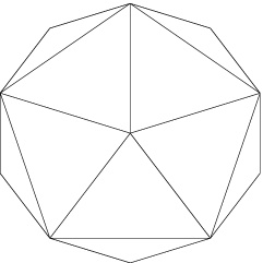
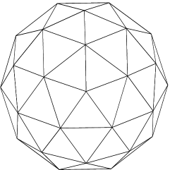
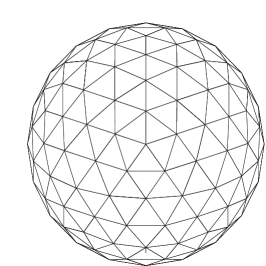
Figure 2: Recursive subdivision (2 levels) of a triangular element

  for all grid index $d$ do

     $E_{d}\leftarrow 0$

     for all microphone pair $ij$ do

        $\tau\leftarrow lookup(d,ij)$

        $E_{d}\leftarrow E_{d}+R^{(e)}_{ij}(\tau)$

     end for

  end for

  direction of source $\leftarrow\textrm{argmax}_{d}\ (E_{d})$

Algorithm 1 Steered beamformer direction search

Once the cross-correlations $R_{ij}^{(e)}(\tau)$ are computed, the search for the best direction on the grid is performed as described by Algorithm 1. The lookup parameter is a pre-computed table of the time delay of arrival (TDOA) for each microphone pair and each direction on the sphere. Using the far-field assumption [8], the TDOA in samples is computed as:

$$\tau_{ij}=\frac{F_{s}}{c}\left(\vec{\mathrm{\mathbf{p}}}_{i}-\mathrm{\vec{\mathrm{\mathbf{p}}}}_{j}\right)\cdot\vec{\mathbf{u}}$$ (12)

where $\vec{\mathrm{\mathbf{p}}}_{i}$ is the position of microphone $i$, $\vec{\mathbf{u}}$ is a unit-vector that points in the direction of the source, $c$ is the speed of sound and $F_{s}$ is the sampling rate. Equation 12 assumes that the time delay is proportional to the distance between the source and microphone. This is only true when there is no diffraction involved. While this hypothesis is only verified for an “open” array (all microphones are in line of sight with the source), in practice we demonstrate experimentally (see Section 6) that the approximation is good enough for our system to work for a “closed” array (in which there are obstacles within the array).

For an array of $M$ microphones and an $N$-element grid, the algorithm requires $M(M-1)N$ table memory accesses and $M(M-1)N/2$ additions. In the proposed configuration ($N=2562$, $M=8$), the accessed data can be made to fit entirely in a modern processor’s L2 cache.

  for $q=1$ to assumed number of sources do

     $D_{q}\leftarrow\textrm{Steered beamformer direction search}$

     for all microphone pair $ij$ do

        $\tau\leftarrow lookup(D_{q},ij)$

        $R^{(e)}_{ij}(\tau)=0$

     end for

  end for

Algorithm 2 Localization of multiple sources

Using Algorithm 1, our system is able to find the loudest source present by maximizing the energy of a steered beamformer. In order to localize other sources that may be present, the process is repeated by removing the contribution of the first source to the cross-correlations, leading to Algorithm 2. Since we do not know how many sources are present, we always look for four sources, as this is the maximum number of sources our beamformer is able to locate at once. This situation leads to a high rate of false detection, even when four or more sources are present. That problem is handled by the particle filter described in Section 5.

4.4 Direction Refining

When a source is located using Algorithm 1, the direction accuracy is limited by the size of the grid used. It is however possible, as an optional step, to further refine the source location estimate. In order to do so, we define a refined grid for the surrounding of the point where a source was found. To take into account the near-field effects, the grid is refined in three dimensions: horizontally, vertically and over distance. Using five points in each direction, we obtain a 125-point local grid with a maximum resolution error of around $1^{\circ}$. For the near-field case, Equation 12 no longer holds, so it is necessary to compute the time differences as:

$$\tau_{ij}=\frac{F_{s}}{c}\left(\left\|d\vec{\mathbf{u}}-\vec{\mathbf{p}}_{j}\right\|-\left\|d\vec{\mathbf{u}}-\vec{\mathbf{p}}_{i}\right\|\right)$$ (13)

where $d$ is the distance between the source and the center of the array. Equation 13 is evaluated for five distances $d$ (ranging from 50 cm to 5 m) in order to find the direction of the source with improved accuracy. Unfortunately, it was observed that the value of $d$ found in the search is too unreliable to provide a good estimate of the distance between the source and the array. The incorporation of the distance nonetheless provides improved accuracy for the near field case.

5 Particle-Based Tracking

The steered beamformer detailed in Section 4 provides only instantaneous, noisy information about sources being possibly present and provides no information about the behavior of the source in time (tracking). For that reason, it is desirable to use a probabilistic temporal integration to track the different sound sources based on all measurements available up to the current time. It has been shown [12, 13, 15] that particle filters are an effective way of tracking sound sources. Using this approach, all hypotheses about the location of each source are represented as a set of particles to which different weights are assigned.

At time $t$, we consider the case of sources $j=0,1,\ldots,M-1$, each modeled using $N$ particles of directions $\mathbf{x}_{j,i}^{(t)}$ and weights $w_{j,i}^{(t)}$. The state vector for the particles is composed of six dimensions, three for position and three for its derivative:

$$\mathbf{s}_{j,i}^{(t)}=\left[\begin{array}[]{c}\mathbf{x}_{j,i}^{(t)}\\ \mathbf{\dot{x}}_{j,i}^{(t)}\end{array}\right]$$ (14)

1. Predict the state $\mathbf{s}_{j}^{(t)}$ from $\mathbf{s}_{j}^{(t-1)}$ for each source $j$

2. Compute instantaneous direction probabilities associated with the steered beamformer response

3. Compute probabilities $P_{q,j}^{(t)}$ associating beamformer peaks to sources being tracked

4. Compute updated particle weights $w_{j,i}^{(t)}$

5. Add or remove sources if necessary

6. Compute source localization estimate $\bar{\mathbf{x}}_{j}^{(t)}$ for each source

7. Resample particles for each source if necessary and go back to step 1.

Algorithm 3 Particle-based tracking algorithm. Steps 1 to 7 correspond to Subsections 5.1 to 5.7.

Since the particle position is constrained to lie on a unit sphere and the speed is tangent to the sphere, there are only four degrees of freedom. The sampling importance resampling (SIR) particle filtering algorithm is outlined in Figure 3 and generalizes sound source tracking to an arbitrary and non-constant number of sources. The probability density function (pdf) for the location of each source is approximated by a set of particles that are given different weights. The weights are updated by taking into account observations obtained from the steered beamformer and by computing the assignment between these observations and the sources being tracked. From there, the estimated location of the source is the weighted mean of the particle positions.

5.1 Prediction

As a predictor, we use the excitation-damping model as proposed in [13] because it has been observed to work well in practice and can easily model different source dynamics only two parameters. The model is defined as:

$$\mathbf{\dot{x}}_{j,i}^{(t)} = a\mathbf{\dot{x}}_{j,i}^{(t-1)}+bF_{\mathbf{x}}$$ (15)

$$\mathbf{x}_{j,i}^{(t)} = \mathbf{x}_{j,i}^{(t-1)}+\Delta T\mathbf{\dot{x}}_{j,i}^{(t)}$$ (16)

where $a=e^{-\alpha\Delta T}$ controls the damping term, $b=\beta\sqrt{1-a^{2}}$ controls the excitation term, $F_{\mathbf{x}}$ is a normally distributed random variable of unit variance and $\Delta T$ is the time interval between updates. We consider three possible states:

• Stationary source ($\alpha=2$, $\beta=0.04$);

• Constant velocity source ($\alpha=0.05$, $\beta=0.2$);

• Accelerated source ($\alpha=0.5$, $\beta=0.2$).

A normalization step ensures that $\mathbf{x}_{i}^{(t)}$ still lies on the unit sphere ($\left\|\mathbf{x}_{j,i}^{(t)}\right\|=1$) after applying Equations 15 and 16.

5.2 Instantaneous Direction Probabilities from Beamformer Response

The steered beamformer described in Section 4 produces an observation $O^{(t)}$ for each time $t$. The observation $O^{(t)}=\left[O_{0}^{(t)}\ldots O_{Q-1}^{(t)}\right]$ is composed of $Q$ potential source locations $\mathbf{y}_{q}$ found by Algorithm 2. We also denote $\mathbf{O}^{(t)}$, the set of all observations $O^{(t)}$ up to time $t$. We introduce the probability $P_{q}$ that the potential source $q$ is a true source (not a false detection). The value of $P_{q}$ can be interpreted as our confidence in the steered beamformer output. We know that the higher the beamformer energy, the more likely a potential source is to be true. For $q>0$, false alarms are very frequent and independent of energy. With this in mind, we define $P_{q}$ empirically as:

$$P_{q}=\left\{\begin{array}[]{ll}\nu^{2}/2,&q=0,\nu\leq 1\\ 1-\nu^{-2}/2,&q=0,\nu>1\\ 0.3,&q=1\\ 0.16,&q=2\\ 0.03,&q=3\end{array}\right.$$ (17)

with $\nu=E_{0}/E_{T}$, where $E_{0}$ is the beamformer output energy for the first source found and $E_{T}$ is a threshold that depends on the number of microphones, the frame size and the analysis window used (we use $E_{T}=150$). Figure 3 shows an example of $P_{q}$ values for potential sources found by the steered beamformer with four people speaking continuously while moving around the microphone array in a moderately reverberant room. Only the azimuth part of $\mathbf{y}_{q}$ is shown as a function of time.

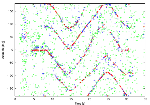
Figure 3: Beamformer output probabilities $P_{q}$ for azimuth as a function of time. Observations with $P_{q}>0.5$ shown in red, $0.2<P_{q}<0.5$ in blue, $P_{q}<0.2$ in green.

At time $t$, the probability density of observing $O_{q}^{(t)}$ for a source located at particle position $\mathbf{x}_{j,i}^{(t)}$ is given by:

$$p\left(\left.O_{q}^{(t)}\right|\mathbf{x}_{j,i}^{(t)}\right)=\mathcal{N}\left(\mathbf{y}_{q};\mathbf{x}_{j,i};\sigma^{2}\right)$$ (18)

where $\mathcal{N}\left(\mathbf{y}_{q};\mathbf{x}_{j,i};\sigma^{2}\right)$ is a normal distribution centered at $\mathbf{x}_{j,i}$ with variance $\sigma^{2}$ evaluated at $\mathbf{y}_{q}$, and models the localization accuracy of the steered beamformer. We use $\sigma=0.05$, which corresponds to an RMS error of 3 degrees for the location found by the steered beamformer. This error takes into account the resolution error (1 degree) as well as other sources of errors, such as noise, reverberation, diffraction, imperfect microphones and errors in microphone placement.

5.3 Probabilities for Multiple Sources

Before we can derive the update rule for the particle weights $w_{j,i}^{(t)}$, we must first introduce the concept of source-observation assignment. For each potential source $q$ detected by the steered beamformer, there are three possibilities:

• It is a false detection ($H_{0}$).

• It corresponds to one of the sources currently tracked ($H_{1}$).

• It corresponds to a new source that is not yet being tracked ($H_{2}$).

In the case of $H_{1}$, we need to determine which tracked source $j$ corresponds to potential source $q$. First, we assume that a potential source may correspond to at most one tracked source and that a tracked source can correspond to at most one potential source.

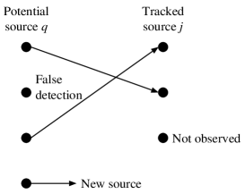
Figure 4: Assignment example where two of the tracked sources are observed, with one new source and one false detection. The assignment can be described as $f(\{0,1,2,3\})=\{1,-2,0,-1\}$.

Let $f:\{0,1,\ldots,Q-1\}\longrightarrow\{-2,-1,0,1,\ldots,M-1\}$ be a function assigning observation $q$ to the source $j$ (values -2 is used for false detection and -1 is used for a new source). Figure 4 illustrates a hypothetical case with four potential sources detected by the steered beamformer and their assignment to the tracked sources. Knowing $P\left(f\left|O^{(t)}\right.\right)$ (the probability that $f$ is the correct assignment given observation $O^{(t)}$) for all possible $f$, we can derive $P_{q,j}$, the probability that the tracked source $j$ corresponds to the potential source $q$ as:

$$P_{q,j}^{(t)} = \sum_{f}\delta_{j,f(q)}P\left(f\left|O^{(t)}\right.\right)$$ (19)

$$P_{q}^{(t)}\left(H_{0}\right) = \sum_{f}\delta_{-2,f(q)}P\left(f\left|O^{(t)}\right.\right)$$ (20)

$$P_{q}^{(t)}\left(H_{2}\right) = \sum_{f}\delta_{-1,f(q)}P\left(f\left|O^{(t)}\right.\right)$$ (21)

where $\delta_{i,j}$ is the Kronecker delta. Equation 19 is in fact the sum of the probabilities of all $f$ that assign potential source $q$ to tracked source $j$ and similarly for Equations 20 and 21.

Omitting $t$ for clarity, the probability $P(f|O)$ is given by:

$$P(f|O)=\frac{p(O|f)P(f)}{p(O)}$$ (22)

Knowing that there is only one correct assignment ($\sum_{f}P(f|O)=1$), we can avoid computing the denominator $p(O)$ by using normalization. Assuming conditional independence of the observations given the mapping function, we can decompose $p\left(\left.O\right|f\right)$ into individual components:

$$p\left(\left.O\right|f\right)=\prod_{q}p\left(\left.O_{q}\right|f(q)\right)$$ (23)

We assume that the distribution of the false detections ($H_{0}$) and the new sources ($H_{2}$) are uniform, while the distribution for tracked sources ($H_{1}$) is the pdf approximated by the particle distribution convolved with the steered beamformer error pdf:

$$p\left(\left.O_{q}\right|f(q)\right)=\left\{\begin{array}[]{ll}1/4\pi,&f(q)=-2\\ 1/4\pi,&f(q)=-1\\ \sum_{i}w_{f(q),i}p\left(\left.O_{q}\right|\mathbf{x}_{j,i}\right),&f(q)\geq 0\end{array}\right.$$ (24)

The a priori probability of $f$ being the correct assignment is also assumed to come from independent individual components, so that:

$$P(f)=\prod_{q}P\left(f(q)\right)$$ (25)

with:

$$P\left(f(q)\right)=\left\{\begin{array}[]{ll}\left(1-P_{q}\right)P_{false},&f(q)=-2\\ P_{q}P_{new}&f(q)=-1\\ P_{q}P\left(Obs_{j}^{(t)}\left|\mathbf{O}^{(t-1)}\right.\right)&f(q)\geq 0\end{array}\right.$$ (26)

where $P_{new}$ is the a priori probability that a new source appears and $P_{false}$ is the a priori probability of false detection. The probability $P\left(Obs_{j}^{(t)}\left|\mathbf{O}^{(t-1)}\right.\right)$ that source $j$ is observable (i.e., that it exists and is active) at time $t$ is given by:

$$P\left(Obs_{j}^{(t)}\left|\mathbf{O}^{(t-1)}\right.\right)=P\left(E_{j}\left|\mathbf{O}^{(t-1)}\right.\right)P\left(\mathrm{A}_{j}^{(t)}\left|\mathbf{O}^{(t-1)}\right.\right)$$ (27)

where $E_{j}$ is the event that source $j$ actually exists and $A_{j}^{(t)}$ is the event that it is active (but not necessarily detected) at time $t$. By active, we mean that the signal it emits is non-zero (for example, a speaker who is not making a pause). The probability that the source exists is given by:

$$P\left(E_{j}\left|\mathbf{O}^{(t-1)}\right.\right)=P_{j}^{(t-1)}+\left(1-P_{j}^{(t-1)}\right)\frac{P_{o}P\left(E_{j}\left|\mathbf{O}^{(t-2)}\right.\right)}{1-\left(1-P_{o}\right)P\left(E_{j}\left|\mathbf{O}^{(t-2)}\right.\right)}$$ (28)

where $P_{o}$ is the a priori probability that a source is not observed (i.e., undetected by the steered beamformer) even if it exists (with $P_{0}=0.2$ in our case) and $P_{j}^{(t)}=\sum_{q}P_{q,j}^{(t)}$ is the probability that source $j$ is observed (assigned to any of the potential sources).

Assuming a first order Markov process, we can write the following about the probability of source activity:

$$P\left(\mathrm{A}_{j}^{(t)}\left|\mathbf{O}^{(t-1)}\right.\right) = P\left(\mathrm{A}_{j}^{(t)}\left|\mathrm{A}_{j}^{(t-1)}\right.\right)P\left(\mathrm{A}_{j}^{(t-1)}\left|\mathbf{O}^{(t-1)}\right.\right)$$ (29)

$$+P\left(\mathrm{A}_{j}^{(t)}\left|\neg\mathrm{A}_{j}^{(t-1)}\right.\right)\left[1-P\left(\mathrm{A}_{j}^{(t-1)}\left|\mathbf{O}^{(t-1)}\right.\right)\right]$$

with $P\left(\mathrm{A}_{j}^{(t)}\left|\mathrm{A}_{j}^{(t-1)}\right.\right)$ the probability that an active source remains active (set to 0.95), and $P\left(\mathrm{A}_{j}^{(t)}\left|\neg\mathrm{A}_{j}^{(t-1)}\right.\right)$ the probability that an inactive source becomes active again (set to 0.05). Assuming that the active and inactive states are equiprobable, the activity probability is computed using Bayes’ rule and usual probability manipulations:

$$P\left(\mathrm{A}_{j}^{(t)}\left|\mathbf{O}^{(t)}\right.\right)=\frac{1}{1+\frac{\left[1-P\left(\mathrm{A}_{j}^{(t)}\left|\mathbf{O}^{(t-1)}\right.\right)\right]\left[1-P\left(\mathrm{A}_{j}^{(t)}\left|O^{(t)}\right.\right)\right]}{P\left(\mathrm{A}_{j}^{(t)}\left|\mathbf{O}^{(t-1)}\right.\right)P\left(\mathrm{A}_{j}^{(t)}\left|O^{(t)}\right.\right)}}$$ (30)

5.4 Weight Update

At times $t$, the new particle weights for source $j$ are defined as:

$$w_{j,i}^{(t)}=p\left(\mathbf{x}_{j,i}^{(t)}\left|\mathbf{O}^{(t)}\right.\right)$$ (31)

Assuming that the observations are conditionally independent given the source position, and knowing that for a given source $j$, $\sum_{i=1}^{N}w_{j,i}^{(t)}=1$, we obtain through Bayesian inference:

$$w_{j,i}^{(t)} = \frac{p\left(\left.\mathbf{O}^{(t)}\right|\mathbf{x}_{j,i}^{(t)}\right)p\left(\mathbf{x}_{j,i}^{(t)}\right)}{p\left(\mathbf{O}^{(t)}\right)}$$ (32)

$$= \frac{p\left(\left.O^{(t)}\right|\mathbf{x}_{j,i}^{(t)}\right)p\left(\left.\mathbf{O}^{(t-1)}\right|\mathbf{x}_{j,i}^{(t)}\right)p\left(\mathbf{x}_{j,i}^{(t)}\right)}{p\left(\mathbf{O}^{(t)}\right)}$$

$$= \frac{p\left(\mathbf{x}_{j,i}\left|O^{(t)}\right.\right)p\left(\mathbf{x}_{j,i}^{(t)}\left|\mathbf{O}^{(t-1)}\right.\right)p\left(O^{(t)}\right)p\left(\mathbf{O}^{(t-1)}\right)}{p\left(\mathbf{O}^{(t)}\right)p\left(\mathbf{x}_{j,i}^{(t)}\right)}$$

$$= \frac{p\left(\mathbf{x}_{j,i}^{(t)}\left|O^{(t)}\right.\right)w_{j,i}^{(t-1)}}{\sum_{i=1}^{N}p\left(\mathbf{x}_{j,i}^{(t)}\left|O^{(t)}\right.\right)w_{j,i}^{(t-1)}}$$

Let $I_{j}^{(t)}$ denote the event that source $j$ is observed at time $t$ and knowing that $P\left(I_{j}^{(t)}\right)=P_{j}^{(t)}=\sum_{q}P_{q,j}^{(t)}$, we have:

$$p\left(\mathbf{x}_{j,i}^{(t)}\left|O^{(t)}\right.\right)=\left(1-P_{j}^{(t)}\right)p\left(\mathbf{x}_{j,i}^{(t)}\left|O^{(t)},\neg I_{j}^{(t)}\right.\right)+P_{j}^{(t)}p\left(\mathbf{x}_{j,i}^{(t)}\left|O^{(t)},I_{j}^{(t)}\right.\right)$$ (33)

In the case where no observation matches the source, all particles have the same probability, so we obtain:

$$p\left(\mathbf{x}_{j,i}^{(t)}\left|O^{(t)}\right.\right)=\left(1-P_{j}^{(t)}\right)\frac{1}{N}+P_{j}\frac{\sum_{q=1}^{Q}P_{q,j}^{(t)}p\left(\left.O_{q}^{(t)}\right|\mathbf{x}_{j,i}^{(t)}\right)}{\sum_{i=1}^{N}\sum_{q=1}^{Q}P_{q,j}^{(t)}p\left(\left.O_{q}^{(t)}\right|\mathbf{x}_{j,i}^{(t)}\right)}$$ (34)

where the denominator on the right side of Equation 34 provides normalization for the $I_{j}^{(t)}$ case, so that $\sum_{i=1}^{N}p\left(\mathbf{x}_{j,i}^{(t)}\left|O^{(t)},I_{j}^{(t)}\right.\right)=1$.

5.5 Adding or Removing Sources

In a real environment, sources may appear or disappear at any moment. If, at any time, $P_{q}(H_{2})$ is higher than a threshold equal to $0.3$, we consider that a new source is present. In that case, a set of particles is created for source $q$. Even when a new source is created, it is only assumed to exist if its probability of existence $P\left(E_{j}\left|\mathbf{O}^{(t)}\right.\right)$ reaches a certain threshold, which we set to 0.98. At this point, the probability of existence is set up 1 and ceases to be updated.

In the same way, we set a time limit on sources. If the source has not been observed ($P_{j}^{(t)}<T_{obs}$) for a certain amount of time, we consider that it no longer exists. In that case, the corresponding particle filter is no longer updated nor considered in future calculations.

5.6 Parameter Estimation

The estimated position of each source is the mean of the pdf and can be obtained as a weighted average of its particles position:

$$\bar{\mathbf{x}}_{j}^{(t)}=\sum_{i=1}^{N}w_{j,i}^{(t)}\mathbf{x}_{j,i}^{(t)}$$ (35)

It is however possible to obtain better accuracy simply by adding a delay to the algorithm. This can be achieved by augmenting the state vector by past position values. At time $t$, the position at time $t-T$ is thus expressed as:

$$\bar{\mathbf{x}}_{j}^{(t-T)}=\sum_{i=1}^{N}w_{j,i}^{(t)}\mathbf{x}_{j,i}^{(t-T)}$$ (36)

Using the same example as in Figure 3 we show in Figure 5 how the particle filter is able to remove the noise and produce smooth trajectories. The added delay produces an even smoother result.

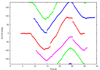
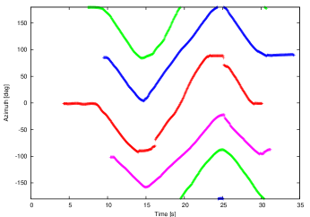
Figure 5: Tracking of four moving sources, showing azimuth as a function of time. Left: no delay, right: delayed estimation (500 ms).

5.7 Resampling

Resampling is performed only when $N_{eff}\approx\left(\sum_{i=1}^{N}w_{j,i}^{2}\right)^{-1}<N_{min}$ [27] with $N_{min}=0.7N$. That criterion ensures that resampling only occurs when new data is available for a certain source. Otherwise, this would cause unnecessary reduction in particle diversity, due to some particles randomly disappearing.

6 Results

The proposed localization system is tested using an array of omni-directional microphones, each composed of an electret cartridge mounted on a simple pre-amplifier. The array is composed of eight microphones, as it is the maximum number of analog input channels on commercially available soundcards. Two array configurations are used for the evaluation of the system. The first configuration (C1) is an open array and consists of inexpensive ($\sim$$1 each) microphones arranged on the summits of a 16 cm cube mounted on top of the Spartacus robot (shown left in Figure 6). The second configuration (C2) is a closed array and uses smaller, middle-range ($\sim$$20 each) microphones, placed through holes at different locations on the body of the robot (shown right in Figure 6). For both arrays, all channels are sampled simultaneously using an RME Hammerfall Multiface DSP connected to a laptop through a CardBus interface. Running the localization system in real-time currently requires 30% of a 1.6 GHz Pentium-M CPU. Due to the low complexity of the particle filtering algorithm, we are able to use 1000 particles per source without noticeable increase in complexity. This also means that the CPU time does not increase significantly with the number of sources present.

 

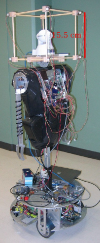
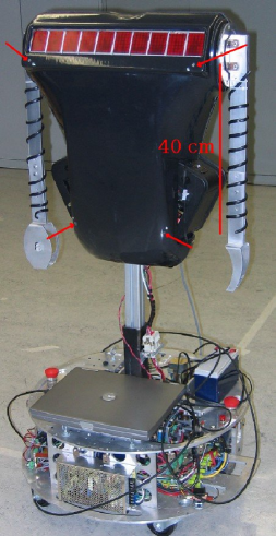
Figure 6: Spartacus robot in configuration C1 (left) and C2 (right).

Experiments are performed in two different environments. The first environment (E1) is a medium-size room (10 m $\times$ 11 m, 2.5 m ceiling) with a reverberation time (-60 dB) of 350 ms. The second environment (E2) is a hall (16 m $\times$ 17 m, 3.1 m ceiling, connected to other rooms) with 1.0 s reverberation time. For all tasks, configurations and environments, all parameters have the same value, except for the reverberation decay $\gamma$, which is set to 0.65 in the E1 environment and 0.85 in the E2 environment.

6.1 Characterization

The system is characterized in environment E1 in terms of detection reliability and accuracy. Detection reliability is defined as the capacity to detect and localize sounds to within 10 degrees, while accuracy is defined as the localization error for sources that are detected. We use three different types of sound: a hand clap, the test sentence “Spartacus, come here”, and a burst of white noise lasting 100 ms. The sounds are played from a speaker placed at different locations around the robot and at three different heights: 0.1 m, 1 m, 1.4 m.

6.1.1 Detection Reliability

Detection reliability is tested at distances (measured from the center of the array) ranging from $1\>\mathrm{m}$ (a normal distance for close interaction) to $7\>\mathrm{m}$ (limitation of the room). Three indicators are computed: correct localization (within 10 degrees), reflections (incorrect elevation due to roof of ceiling), and other errors. For all indicators, we compute the number of occurrences divided by the number of sounds played. This test includes 1440 sounds at a 22.5^∘ interval for 1 m and 3 m and 360 sounds at a 90^∘ interval for 5 m and 7 m. Because of the limited size of the room used for the experiment, the tests for 5 m and 7 m had to use fixed positions for the robot and the source, leading to less variability in the conditions. This can explain differences between these results and those obtained for shorted distances, especially for reflections.

Results are shown in Table 1 for both C1 and C2 configurations. In configuration C1, results show near-perfect reliability even at seven meter distance. For C2, we noted that the reliability depends on the sound type, so detailed results for different sounds are provided in Table 2, showing that only hand clap sounds cannot be reliably detected passed one meter. We expect that a human would have achieved a score of 100% for this reliability test.

Like most localization algorithms, our system is unable to detect pure tones. This behavior is explained by the fact that sinusoids occupy only a very small region of the spectrum and thus have a very small contribution to the cross-correlations with the proposed weighting. It must be noted that tones tend to be more difficult to localize even for the human auditory system.

Table 1: Detection reliability for C1 and C2 configurations

Distance	Correct (%)		Reflection (%)		Other error (%)
	C1	C2	C1	C2	C1	C2
1 m	100	94.2	0.0	7.3	0.0	1.3
3 m	99.4	80.6	0.0	21.0	0.3	0.1
5 m	98.3	89.4	0.0	0.0	0.0	1.1
7 m	100	85.0	0.6	1.1	0.6	1.1

Table 2: Correct localization rate as a function of sound type and distance for C2 configuration

Distance	Hand clap (%)	Speech (%)	Noise burst (%)
1 m	88.3	98.3	95.8
3 m	50.8	97.9	92.9
5 m	71.7	98.3	98.3
7 m	61.7	95.0	98.3

6.1.2 Localization Accuracy

In order to measure the accuracy of the localization system, we use the same setup as for measuring reliability, with the exception that only distances of $1\>\mathrm{m}$ and $3\>\mathrm{m}$ are tested (1440 sounds at a 22.5^∘ interval) due to limited space available in the testing environment. Neither distance nor sound type has significant impact on accuracy. The root mean square accuracy results are shown in Table 3 for configurations C1 and C2. Both azimuth and elevation are shown separately. According to [28, 29], human sound localization accuracy ranges between two and four degrees in similar conditions. The localization accuracy of our system is thus equivalent or better than human localization accuracy.

Table 3: Localization accuracy (root mean square error)

Localization error	C1 (deg)	C2 (deg)
Azimuth	1.10	1.44
Elevation	0.89	1.41

6.2 Source Tracking

We measure the tracking capabilities of the system for multiple sound sources. These are performed using the C2 configuration in both E1 and E2 environments. In all cases, the distance between the robot and the sources is approximately two meters. The azimuth is shown as a function of time for each source. The elevation is not shown as it is almost the same for all sources during these tests. The trajectories for the three experiments are shown in Figure 7.

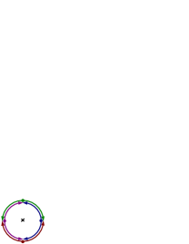
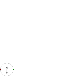
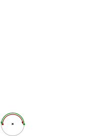
Figure 7: Source trajectories (robot represented as an X). Left: moving sources. Center: moving robot. Right: sources with intersecting trajectories.

6.2.1 Moving Sources

In a first experiments, four people were told to talk continuously (reading a text with normal pauses between words) to the robot while moving, as shown on the left of Figure 7. Each person walked 90 degrees towards the left of the robot before walking 180 degrees towards the right.

Results are presented in Figure 8 for delayed estimation (500 ms). In both environments, the source estimated trajectories are consistent with the trajectories of the four speakers and only one false detection was present (in E1, at $t=15\>\mathrm{s}$) for a short period of time.

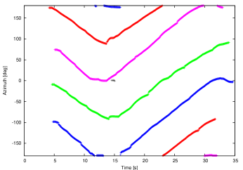
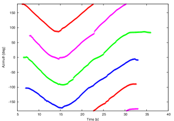
Figure 8: Four speakers moving around a stationary robot. Left: E1, right: E2. False detection shown in black.

6.2.2 Moving Robot

Tracking capabilities of our system are also evaluated in the context where the robot is moving, as shown in the center of Figure 7. In this experiment, two people are talking continuously to the robot as it is passing between them. The robot then makes a half-turn to the left. Results are presented in Figure 9 for delayed estimation (500 ms). Once again, the estimated source trajectories are consistent with the trajectories of the sources relative to the robot for both environments. Only one false detection was present (in E1, at $t=38\>\mathrm{s}$) for a short period of time.

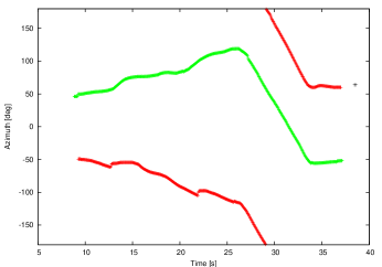
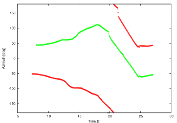
Figure 9: Two stationary speakers with the robot moving. Left: E1, right: E2. False detection shown in black.

6.2.3 Sources with Intersecting Trajectories

In this experiment, two moving speakers are talking continuously to the robot, as shown on the right of Figure 7. They start from each side of the robot, intersecting in front of the robot before reaching the other side. Results in Figure 10 show that the particle filter is able to keep track of each source. This result is possible because the prediction step imposes some inertia to the sources and despite the fact that the steered beamformer typically only “sees” one source when the two sources are very close.

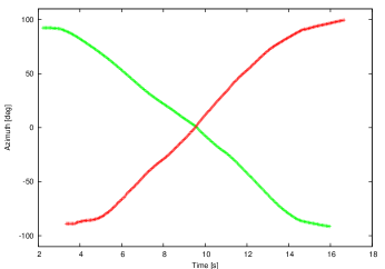
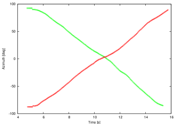
Figure 10: Two speakers intersecting in front of the robot. Left: E1, right: E2.

6.2.4 Number of Microphones

These results evaluate how the number of microphones used affect the system capabilities. To do so, we use the same recording as in 6.2.1 for C2 in E1 with only a subset of the microphone signals to perform localization. Since a minimum of four microphones are necessary for localizing sounds without ambiguity, we evaluate the system for four to seven microphones (selected arbitrarily as microphones number $1$ through $N$). Comparing results of Figure 11 to those obtained in Figure 8 for E1, it can be observed that tracking capabilities degrade gracefully as microphones are removed. While using seven microphones makes little difference compared to the baseline of eight microphones, the system is unable to reliably track more than two of the sources when only four microphones are used. Although there is no theoretical relationship between the number of microphones and the maximum number of sources that can be tracked, this clearly shows the how redundancy added by using more microphones can help in the context of sound source localization.

Figure 11: Tracking of four sources using C2 in the E1 environment, using 4 to 7 microphones.

6.3 Localization and Tracking for Robot Control

This experiment is performed in real-time and consists of making the robot follow the person speaking to it. At any time, only the source present for the longest time is considered. When the source is detected in front (withing 10 degrees) of the robot, it is made to go forward. At the same time, regardless of the angle, the robot turns toward the source in such a way as to keep the source in front. Using this simple control system, it is possible to control the robot simply by talking to it, even in noisy and reverberant environments.

This has been tested by controlling the robot going from environment E1 to environment E2, having to go through corridors and an elevator, speaking to the robot with normal intensity at a distance ranging from one meter to three meters. The system worked in real-time, providing tracking data at a rate of 25 Hz (no additional delay on the estimator) with the robot reaction time limited mainly by the inertia of the robot. One problem we encountered during the experiment is that when going through corridors, the robot would sometimes mistake reflections on the walls for real sources. Fortunately, the fact that the robot considers only the oldest source present reduces problems from both reflections and noise sources.

7 Conclusion

Using an array of eight microphones, we have implemented a system that is able to localize and track simultaneous moving sound sources in the presence of noise and reverberation, at distances up to seven meters. We have also demonstrated that the system is capable of controlling in real-time the motion of a robot, using only the direction of sounds. The tracking capabilities demonstrated result from combining our frequency-domain steered beamformer with a particle filter tracking multiple sources. Moreover, the original solution we found to the source-observation assignment problem is also applicable to other multiple objects tracking problems. Other novelties in this paper include the frequency-domain implementation of our steered beamformer and the way we make it robust to reverberation.

A robot using the proposed system has access to a rich, robust and useful set of information derived from its acoustic environment. This can certainly affect its ability of making autonomous decisions in real life settings, and show higher intelligent behavior. Also, because the system is able to localize multiple sound sources, it can be exploited by a sound separation algorithm and enable speech recognition to be performed. This will allow to identify the localized sound sources so that additional relevant information can be obtained from the acoustic environment.

References

- [1] M. Marschark, Raising and Educating a Deaf Child, Oxford University Press, 1998, http://www.rit.edu/ memrtl/course/interpreting/modules/modulelist.htm.
- [2] W. M. Hartmann, How we localize sounds, Physics Today (1999) 24–29.
- [3] J.-M. Valin, F. Michaud, B. Hadjou, J. Rouat, Localization of simultaneous moving sound sources for mobile robot using a frequency-domain steered beamformer approach, in: Proceedings IEEE International Conference on Robotics and Automation, Vol. 1, 2004, pp. 1033–1038.
- [4] B. Mungamuru, P. Aarabi, Enhanced sound localization, IEEE Transactions on Systems, Man, and Cybernetics Part B 34 (3) (2004) 1526–1540.
- [5] K. Nakadai, D. Matsuura, H. G. Okuno, H. Kitano, Applying scattering theory to robot audition system: Robust sound source localization and extraction, in: Proceedings IEEE/RSJ International Conference on Intelligent Robots and Systems, 2003, pp. 1147–1152.
- [6] K. Nakadai, T. Lourens, H. G. Okuno, H. Kitano, Active audition for humanoid, in: Proceedings of the Seventeenth National Conference on Artificial Intelligence (AAAI), 2000, pp. 832–839.
- [7] F. Asano, M. Goto, K. Itou, H. Asoh, Real-time source localization and separation system and its application to automatic speech recognition, in: Proc. EUROSPEECH, 2001, pp. 1013–1016.
- [8] J.-M. Valin, F. Michaud, J. Rouat, D. Létourneau, Robust sound source localization using a microphone array on a mobile robot, in: Proceedings IEEE/RSJ International Conference on Intelligent Robots and Systems, 2003, pp. 1228–1233.
- [9] S. Kagami, Y. Tamai, H. Mizoguchi, T. Kanade, Microphone array for 2D sound localization and capture, in: Proceedings IEEE International Conference on Robotics and Automation, 2004, pp. 703–708.
- [10] D. Bechler, M. Schlosser, K. Kroschel, System for robust 3D speaker tracking using microphone array measurements, in: Proceedings IEEE/RSJ International Conference on Intelligent Robots and Systems, 2004, pp. 2117–2122.
- [11] M. S. Arulampalam, S. Maskell, N. Gordon, T. Clapp, A tutorial on particle filters for online nonlinear/non-gaussian bayesian tracking, IEEE Transactions on Signal Processing 50 (2) (2002) 174–188.
- [12] D. B. Ward, R. C. Williamson, Particle filtering beamforming for acoustic source localization in a reverberant environment, in: Proceedings IEEE International Conference on Acoustics, Speech, and Signal Processing, Vol. II, 2002, pp. 1777–1780.
- [13] D. B. Ward, E. A. Lehmann, R. C. Williamson, Particle filtering algorithms for tracking an acoustic source in a reverberant environment, IEEE Transactions on Speech and Audio Processing 11 (6).
- [14] J. Vermaak, A. Blake, Nonlinear filtering for speaker tracking in noisy and reverberant environments, in: Proceedings IEEE International Conference on Acoustics, Speech, and Signal Processing, Vol. 5, 2001, pp. 3021–3024.
- [15] H. Asoh, F. Asano, K. Yamamoto, T. Yoshimura, Y. Motomura, N. Ichimura, I. Hara, J. Ogata, An application of a particle filter to bayesian multiple sound source tracking with audio and video information fusion, in: Proceedings of 7th International Conference on Information Fusion, 2004, pp. 805–812.
- [16] J. Vermaak, A. Doucet, P. Pérez, Maintaining multi-modality through mixture tracking, in: Proceedings International Conference on Computer Vision (ICCV), 2003, pp. 1950–1954.
- [17] J. MacCormick, A. Blake, A probabilistic exclusion principle for tracking multiple objects, International Journal of Computer Vision 39 (1) (2000) 57–71.
- [18] C. Hue, J.-P. L. Cadre, P. Perez, A particle filter to track multiple objects, in: Proceedings IEEE Workshop on Multi-Object Tracking, 2001, pp. 61–68.
- [19] J. Vermaak, S. Godsill, P. Pérez, Monte carlo filtering for multi-target tracking and data association, IEEE Transactions on Aerospace and Electronic Systems.
- [20] R. Duraiswami, D. Zotkin, L. Davis, Active speech source localization by a dual coarse-to-fine search, in: Proceedings IEEE International Conference on Acoustics, Speech, and Signal Processing, 2001, pp. 3309–3312.
- [21] M. Omologo, P. Svaizer, Acoustic event localization using a crosspower-spectrum phase based technique, in: Proceedings IEEE International Conference on Acoustics, Speech, and Signal Processing, 1994, pp. II–273–II–276.
- [22] Y. Ephraim, D. Malah, Speech enhancement using minimum mean-square error short-time spectral amplitude estimator, IEEE Transactions on Acoustics, Speech and Signal Processing ASSP-32 (6) (1984) 1109–1121.
- [23] I. Cohen, B. Berdugo, Speech enhancement for non-stationary noise environments, Signal Processing 81 (2) (2001) 2403–2418.
- [24] J. Huang, N. Ohnishi, N. Sugie, Sound localization in reverberant environment based on the model of the precedence effect, IEEE Transactions on Instrumentation and Measurement 46 (4) (1997) 842–846.
- [25] J. Huang, N. Ohnishi, X. Guo, N. Sugie, Echo avoidance in a computational model of the precedence effect, Speech Communication 27 (3-4) (1999) 223–233.
- [26] F. Giraldo, Lagrange-galerkin methods on spherical geodesic grids, Journal of Computational Physics 136 (1997) 197–213.
- [27] A. Doucet, S. Godsill, C. Andrieu, On sequential Monte Carlo sampling methods for bayesian filtering, Statistics and Computing 10 (2000) 197–208.
- [28] W. M. Hartmann, Localization of sounds in rooms, Journal of the Acoustical Society of America 74 (1983) 1380–1391.
- [29] B. Rakerd, W. M. Hartmann, Localization of noise in a reverberant environment, in: Proceedings International Congress on Acoustics, 2004.