AA-stacked Bilayer Graphene Quantum Dots in Magnetic Field

Abdelhadi Belouad^a, Youness Zahidi^a and Ahmed Jellal^a,b

^aTheoretical Physics Group, Faculty of Sciences, Chouaïb Doukkali University,

PO Box 20, 24000 El Jadida, Morocco

^bSaudi Center for Theoretical Physics, Dhahran, Saudi Arabia

Dedicated to Prof. Dr. Hachim A. Yamani on the occasion of his 70th birthday

By applying the infinite-mass boundary condition, we analytically calculate the confined states and the corresponding wave functions of AA-stacked bilayer graphene quantum dots in the presence of an uniform magnetic field $B$. It is found that the energy spectrum shows two set of levels, which are the double copies of the energy spectrum for single layer graphene, shifted up-down by $+\gamma$ and $-\gamma$, respectively. However, the obtained spectrum exhibits different symmetries between the electron and hole states as well as the intervalley symmetries. It is noticed that, the applied magnetic field breaks all symmetries, except one related to the intervalley electron-hole symmetry, i.e. $E^{e}(\tau,m)=-E^{h}(\tau,m)$. Two different regimes of confinement are found: the first one is due to the infinite-mass barrier at weak $B$ and the second is dominated by the magnetic field as long as $B$ is large. We numerically investigated the basics features of the energy spectrum to show the main similarities and differences with respect to monolayer graphene, AB-stacked bilayer graphene and semiconductor quantum dots.

PACS numbers: 81.05.ue, 81.07.Ta, 73.22.Pr
Keywords: AA-stacked bilayer graphene, quantum dot, infinite-mass, magnetic field.

1 Introduction

Graphene [1, 2] is the name given to the atomically thin layer of carbon atoms that can be viewed either as a single layer of graphite or an unrolled nanotube. The experimental breakthrough [1], has generated much excitement in the condensed matter physics community. The large interest is due to both the unusual mechanical and electronic properties as well as for the prospects of applications, which may lead to their use in novel nanoelectronic devices. Graphene can provide a good platform for the study of the electronic properties of a pure two-dimensional system. In fact, graphene has an unique band structure, which is gapless and exhibits a linear dispersion relation at two inequivalent points, labeled as $K$ and $K^{\prime}$ in the Brillouin zone. In addition, graphene presents a variety of exotic electronic properties like electron-hole symmetry [3], Klein tunneling [4] and anomalous quantum Hall effect [5]. The equation describing the electronic excitations in graphene is formally similar to the Dirac equation for massless fermions, which travel at a speed of the order of $v_{F}\approx 10^{6}$ $m/s$ [6, 7].

Graphene can not only exist in the free state, but two or more layers can stack above each other to form what is called few layer graphene. As example the bilayer graphene (BLG) that is the stack of two sheets. There are two dominant ways in which the two layers can be stacked. The first one is the so called AB-stacked BLG [8, 9] and the second is the AA-stacked BLG [10, 11]. In the case of AB-stacked BLG, only one atom in the lower layer lies directly below an other atom in the upper layer and the other two atoms over the center of the hexagon in the other layer. However, for AA-stacked BLG the A sublattice of the top layer is stacked directly above the same sublattice of the bottom layer. The BLG exhibits additional properties that can not be found in single layer graphene. Indeed, the AB-stacked BLG has a gapless quadratic dispersion relation, two conduction bands and two valance bands, each pair is separated by an interlayer coupling energy of order $\gamma_{1}=400\ meV$. However, the energy bands for AA-stacked BLG are just the double copies of single layer graphene bands shifted up and down by the interlayer coupling $\gamma=200\ meV$.

Graphene quantum dots (QDs) [12, 13, 14] have sparked intense research activities related to quantum information storage and realization of a system based on the QD. The Klein tunneling effect [4] in graphene prevents carrier confinement and thus prevents the realization of QDs in graphene [13, 14]. From an application technological point of view, the confinement of electrons is of particular importance to build functional nano-devices. Hence, manufacturing graphene based electronic devices will be a great challenge [15, 14]. Several studies showed that the confinement of carriers can be made whether, through an external magnetic field [16] or finite mass term with an electrostatic potential [17]. Recently, the energy levels of circular graphene QDs in the presence and absence of a external magnetic field, was investigated, for the infinite-mass and zigzag boundary conditions [18]. Moreover, theoretical studies were reported on circular, triangular and hexagonal graphene QDs for different boundary conditions in the presence of a perpendicular magnetic field [19, 20, 21, 22].

In this paper, we consider a circular QD in AA-stacked bilayer graphene in the presence of an external magnetic field. We solve the Dirac equation in the barrier region (region II) and apply the boundary conditions, for the four wave function components on the solid circles shown in Figure 2 for the limit $V\longrightarrow\infty$, to end up with the infinite mass boundary condition. For this, we start with the system shown in Figure 2(a) and match the wave function components in regions I and III as well as make use of the appropriate approximations. Subsequently, we obtain the energy levels for circular QDs in AA-stacked BLG corresponding to both valleys $K$ and $K^{\prime}$ in terms of the dot radius and the magnetic field. We investigate the basic features of our results and compare them with those for circular QDs in monolayer graphene and AB-stacked BLG.

The present paper is organized as follows. In section $2$, we formulate our problem by setting the theoretical model that is relevant to describe our system. Subsequently, we use the eigenvalue equation to explicitly determine the infinite mass boundary conditions. This will be employed, in section 3, to separately study the energy spectrum of our system in the absence and presence of the magnetic field. To underline the behavior of our system we numerically investigate the basic features of the obtained results in section $4$. In the final section, we conclude our results.

2 Problem setting

To set our problem, let us consider a bilayer graphene system consists of two monolayers, arranged in the Bernal AA stacking way. Each layer consists of two triangular sublattices, labeled A and B (upper layer) and A${}^{{}^{\prime}}$ and B${}^{{}^{\prime}}$ (lower layer). The A sublattice of the upper layer is stacked directly above the same sublattice of the lower layer by the interlayer coupling $\gamma=200\ meV$ [23] as presented in Figure 1.

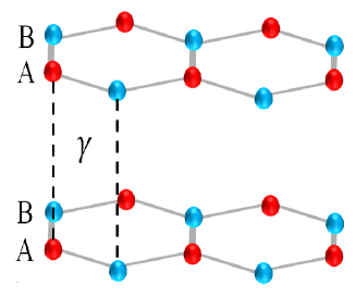
Figure 1: Schematic illustration of lattice structure of AA-stacked bilayer graphene. It is consists of two graphene layers. Each carbon atom of the upper layer is located above the corresponding atom of the lower layer and they are separated by an interlayer coupling energy $\gamma$. The unit cell of the AA-stacked bilayer graphene consists of four atoms A, B, A’ and B’.

Next, we assume that the carriers in AA-stacked bilayer graphene are confined in a circular area of radius $R$, which can be modeled by an infinite-mass barrier. For this, we will derive the infinite-mass boundary conditions for the Dirac electron interacting with circular barrier structures as shown in blue color (Figure 2), in the presence of a perpendicular magnetic field. More precisely, Figure 2 illustrates a schematic depiction of the mass barrier profile for an AA-stacked BLG quantum dots that will be used to deal with different issues.

(a)

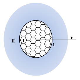
(b)

Figure 2: Illustration of the mass barrier profile. (2(a)): a ring-shaped barrier. (2(b)): circular quantum dot, made of AA-stacked bilayer graphene surrounded by an infinite-mass barrier.

To be much more concrete, we consider only nearest neighbor in-plane hopping, as well as direct interlayer hopping, i.e. A to A${}^{{}^{\prime}}$ or B to B${}^{{}^{\prime}}$ sublattices. Then, in the basis of $\Psi=\left(\Psi_{A},\ \Psi_{B},\ \Psi_{B^{{}^{\prime}}},\ \Psi_{A^{{}^{\prime}}}\right)^{T}$, where $\Psi_{A\ (A^{{}^{\prime}})}$ and $\Psi_{B\ (B^{{}^{\prime}})}$ are the envelope functions associated with the probability amplitudes of the wave functions on the A (A${}^{{}^{\prime}}$) and B (B${}^{{}^{\prime}}$) sublattices of the upper (lower) layer, the Hamiltonian describing our system is given by

$$H=\begin{pmatrix}\tau V(r)&\pi&0&\gamma\\ \pi^{\dagger}&-\tau V(r)&\gamma&0\\ 0&\gamma&\tau V(r)&\pi^{\dagger}\\ \gamma&0&\pi&-\tau V(r)\end{pmatrix}$$ (1)

where the momentum operators in polar coordinates

$$\pi=-i\hbar v_{F}e^{i\theta}\left(\frac{\partial}{\partial r}+\frac{i}{r}\frac{\partial}{\partial\theta}\right),\qquad\pi^{\dagger}=-i\hbar v_{F}e^{-i\theta}\left(\frac{\partial}{\partial r}-\frac{i}{r}\frac{\partial}{\partial\theta}\right)$$ (2)

$v_{F}\approx 10^{6}m/s$ is the Fermi velocity and $\tau=\pm$ differentiates the two valleys $K$ and $K^{\prime}$. The mass profile $V(r)$ is considered to be circularly symmetric

$$V(r)=\left\{\begin{array}[]{cc}0,&\;r<R\\ \infty,&\;r>R\end{array}\right.$$ (3)

and $r$ is the radial coordinate of the polar coordinates and $R$ is the radius of the quantum dot. Since the total angular momentum operator $J_{z}$ commutes with $H$, then we can construct a common basis in terms of the eigenspinors, such as

$$\Psi(r,\theta)=\begin{pmatrix}\Phi_{A}(r)e^{im\theta}\\ i\Phi_{B}(r)e^{i(m-1)\theta}\\ i\Phi_{B^{\prime}}(r)e^{i(m-1)\theta}\\ \Phi_{A^{\prime}}e^{im\theta}\end{pmatrix}$$ (4)

where $m$ is the angular momentum quantum number, which being an integer. It is convenient to switch to the dimensionless variables by setting the quantities

$$\frac{r}{R}\longrightarrow r,\qquad\frac{R}{\hbar v_{F}}E\longrightarrow E,\qquad\frac{R}{\hbar v_{F}}\gamma\longrightarrow\gamma,\qquad\frac{R}{\hbar v_{F}}V\longrightarrow V.$$ (5)

Plugging (4) into the eigenvalue equation $H\Psi(r,\theta)=E\Psi(r,\theta)$, to obtain the following coupled differential equations

$$\left(\frac{\partial}{\partial r}+\frac{m}{r}\right)\Phi_{A}(r)=-(E+\tau V)\Phi_{B}(r)+\gamma\Phi_{B^{\prime}}(r)$$ (6a)

$$\left(\frac{\partial}{\partial r}-\frac{m-1}{r}\right)\Phi_{B}(r)=(E-\tau V)\Phi_{A}(r)-\gamma\Phi_{A^{\prime}}(r)$$ (6b)

$$\left(\frac{\partial}{\partial r}-\frac{m-1}{r}\right)\Phi_{B^{\prime}}(r)=(E+\tau V)\Phi_{A^{\prime}}(r)-\gamma\Phi_{A}(r)$$ (6c)

$$\left(\frac{\partial}{\partial r}+\frac{m}{r}\right)\Phi_{A^{\prime}}(r)=-(E-\tau V)\Phi_{B^{\prime}}(r)+\gamma\Phi_{B}(r).$$ (6d)

Before getting the solutions of the energy spectrum, we first look for the infinite-mass boundary condition for AA-stacked bilayer graphene. This can be done by solving the differential equations (6) in the barrier region (region II). Indeed, we consider the ring-shaped barrier shown in Figure 2(2(a)) and take the limit $V\longrightarrow\infty$ to end up with the approximate set of differential equations

$$\frac{\partial}{\partial r}\Phi_{A}(r)=-\tau V\Phi_{B}(r)+\gamma\Phi_{B^{\prime}}(r)$$ (7a)

$$\frac{\partial}{\partial r}\Phi_{B}(r)=-\tau V\Phi_{A}(r)-\gamma\Phi_{A^{\prime}}(r)$$ (7b)

$$\frac{\partial}{\partial r}\Phi_{B^{\prime}}(r)=\tau V\Phi_{A^{\prime}}(r)-\gamma\Phi_{A}(r)$$ (7c)

$$\frac{\partial}{\partial r}\Phi_{A^{\prime}}(r)=\tau V\Phi_{B^{\prime}}(r)+\gamma\Phi_{B}(r).$$ (7d)

These give the eigenspinor solution in the thin shadowed region II, delimited by two circles of radius $1\pm\delta$ with the condition $\delta\ll 1$, such as

$$\Phi_{A}(r)=ae^{(r-1)\alpha_{+}}+be^{-(r-1)\alpha_{+}}+ce^{(r-1)\alpha_{-}}+de^{-(r-1)\alpha_{-}}$$ (8a)

$$\Phi_{B}(r)=\frac{-\tau}{V}\left(\alpha_{+}ae^{(r-1)\alpha_{+}}-\alpha_{+}be^{-(r-1)\alpha_{+}}+\alpha_{-}ce^{(r-1)\alpha_{-}}-\alpha_{-}de^{-(r-1)\alpha_{-}}\right)$$ (8b)

$$\Phi_{B^{\prime}}(r)=\frac{i}{V}\left(\alpha_{+}ae^{(r-1)\alpha_{+}}-\alpha_{+}be^{-(r-1)\alpha_{+}}-\alpha_{-}ce^{(r-1)\alpha_{-}}+\alpha_{-}de^{-(r-1)\alpha_{-}}\right)$$ (8c)

$$\Phi_{A^{\prime}}(r)=i\tau\left(ae^{(r-1)\alpha_{+}}+be^{-(r-1)\alpha_{+}}-ce^{(r-1)\alpha_{-}}-de^{-(r-1)\alpha_{-}}\right)$$ (8d)

where the parameter $\alpha$ is defined by

$$\alpha^{2}_{\pm}=(V\pm i\gamma)^{2}$$ (9)

and the coefficients ($a,b,c,d$) are constants. Using the continuity of the wave functions at the boundary conditions on the two circles to obtain the solutions at the boundary $1-\delta$

$$\Phi^{\text{I}}_{A}(1-\delta)=ae^{-\delta\alpha_{+}}+be^{\delta\alpha_{+}}+ce^{-\delta\alpha_{-}}+de^{\delta\alpha_{-}}$$ (10a)

$$\Phi^{\text{I}}_{B}(1-\delta)=\frac{-\tau}{V}\left(\alpha_{+}ae^{-\delta\alpha_{+}}-\alpha_{+}be^{\delta\alpha_{+}}+\alpha_{-}ce^{-\delta\alpha_{-}}-\alpha_{-}de^{\delta\alpha_{-}}\right)$$ (10b)

$$\Phi^{\text{I}}_{B^{\prime}}(1-\delta)=\frac{i}{V}\left(\alpha_{+}ae^{-\delta\alpha_{+}}-\alpha_{+}be^{\delta\alpha_{+}}-\alpha_{-}ce^{-\delta\alpha_{-}}+\alpha_{-}de^{\delta\alpha_{-}}\right)$$ (10c)

$$\Phi^{\text{I}}_{A^{\prime}}(1-\delta)=i\tau\left(ae^{-\delta\alpha_{+}}+be^{\delta\alpha_{+}}-ce^{-\delta\alpha_{-}}-de^{\delta\alpha_{-}}\right)$$ (10d)

as well as at $1+\delta$

$$\Phi^{\text{III}}_{A}(1+\delta)=ae^{\delta\alpha_{+}}+be^{-\delta\alpha_{+}}+ce^{\delta\alpha_{-}}+de^{-\delta\alpha_{-}}$$ (11a)

$$\Phi^{\text{III}}_{B}(1+\delta)=\frac{-\tau}{V}\left(\alpha_{+}ae^{\delta\alpha_{+}}-\alpha_{+}be^{-\delta\alpha_{+}}+\alpha_{-}ce^{\delta\alpha_{-}}-\alpha_{-}de^{-\delta\alpha_{-}}\right)$$ (11b)

$$\Phi^{\text{III}}_{B^{\prime}}(1+\delta)=\frac{i}{V}\left(\alpha_{+}ae^{\delta\alpha_{+}}-\alpha_{+}be^{-\delta\alpha_{+}}-\alpha_{-}ce^{\delta\alpha_{-}}+\alpha_{-}de^{-\delta\alpha_{-}}\right)$$ (11c)

$$\Phi^{\text{III}}_{A^{\prime}}(1+\delta)=i\tau\left(ae^{\delta\alpha_{+}}+be^{-\delta\alpha_{+}}-ce^{\delta\alpha_{-}}-de^{-\delta\alpha_{-}}\right).$$ (11d)

At the boundary on the two circles demarcating the region II, the four-component wave-functions should be continuous. Connecting the wave-function components in regions I and III and taking into account $\delta\ll 1$ to write

$$\Phi^{\text{III}}_{B^{\prime}}(1)-\Phi^{\text{I}}_{B^{\prime}}(1) = -i\tau\left(\Phi^{\text{III}}_{B}(1)-\Phi^{\text{I}}_{B}(1)\right)$$

$$+\frac{\tau\alpha_{-}}{V}\tanh(\delta\alpha_{-})\left[\Phi^{\text{III}}_{A^{\prime}}(1)+\Phi^{\text{I}}_{A^{\prime}}(1)-i\tau\left(\Phi^{\text{III}}_{A}(1)+\Phi^{\text{I}}_{A}(1)\right)\right]$$

$$\Phi^{\text{III}}_{A^{\prime}}(1)-\Phi^{\text{I}}_{A^{\prime}}(1) = -i\tau\left(\Phi^{\text{III}}_{A}(1)-\Phi^{\text{I}}_{A}(1)\right)$$

$$-\frac{V}{\alpha_{+}}\tanh(\delta\alpha_{+})\left[i\left(\Phi^{\text{III}}_{B}(1)+\Phi^{\text{I}}_{B}(1)\right)-\tau(\Phi^{\text{III}}_{B^{\prime}}(1)+\Phi^{\text{I}}_{B^{\prime}}(1))\right].$$

To find the general form of the boundary conditions corresponding to the ring-shaped barrier shown in Figure 2(2(a)), we consider the limits $\delta\longrightarrow 0,V\gg\gamma$ and $\tanh(\delta\alpha_{\pm})=q$, where $q$ is a function of the height of the barrier $V$. Thus (2) and (2) become

$$\Phi^{\text{III}}_{B^{\prime}}(1)-\Phi^{\text{I}}_{B^{\prime}}(1)=-i\tau\left(\Phi^{\text{III}}_{B}(1)-\Phi^{\text{I}}_{B}(1)\right)+q\left[\tau(\Phi^{\text{III}}_{A^{\prime}}(1)+\Phi^{\text{I}}_{A^{\prime}}(1))-i\left(\Phi^{\text{III}}_{A}(1)+\Phi^{\text{I}}_{A}(1)\right)\right]$$ (14)

$$\Phi^{\text{III}}_{A^{\prime}}(1)-\Phi^{\text{I}}_{A^{\prime}}(1)=-i\tau\left(\Phi^{\text{III}}_{A}(1)-\Phi^{\text{I}}_{A}(1)\right)+q\left[\tau(\Phi^{\text{III}}_{B^{\prime}}(1)+\Phi^{\text{I}}_{B^{\prime}}(1))-i\left(\Phi^{\text{III}}_{B}(1)+\Phi^{\text{I}}_{B}(1)\right)\right].$$ (15)

We can also derive the boundary condition for the structure shown in Figure 2(2(b)). Indeed, we consider the limits: $V\longrightarrow\infty$, $q=1$ and $\Phi^{\text{III}}_{A^{\prime}}(1)=\Phi^{\text{III}}_{B^{\prime}}(1)=\Phi^{\text{III}}_{A}(1)=\Phi^{\text{III}}_{B}(1)=0$, to end up with the boundary conditions for an AA-stacked bilayer quantum dot surrounded by an infinite-mass barrier

$$\Phi^{\text{I}}_{B}(1)-\tau\Phi^{\text{I}}_{A}(1)=0$$ (16a)

$$\Phi^{\text{I}}_{B^{\prime}}(1)+\tau\Phi^{\text{I}}_{A^{\prime}}(1)=0.$$ (16b)

It is important to note that the infinite-mass boundary condition (16) is depending only to the region I, which means that the region outside the dot (region II) is forbidden for particles [7]. In addition, (16a) and (16b) have the same structure except for a sign, each one of them connects the value of the pseudospin components at the boundary of the two sublattices of each layer separately. In contrast of those obtained for AB-stacked bilayer graphene, were they connect each layer to the other[19]. We observe also that each one of these two conditions ((16a) and (16b)) has the same form to that obtained in the case of monolayer graphene [18]. Note that from both conditions we find the energy spectrum, which will be discussed in the next section.

3 Energy spectrum

We will look for the solutions of the energy spectrum inside the quantum dot by using the obtained infinite-mass boundary conditions. In doing so, we separately consider the cases of the absence and presence of a magnetic field.

3.1 Zero magnetic field

Let us in the beginning investigate the situation where the magnetic filed is switched off and underline the behavior of our system. Indeed, (6) for $V=0$ gives

$$\left(\frac{\partial}{\partial r}+\frac{m}{r}\right)\Phi_{A}(r)=-E\Phi_{B}(r)+\gamma\Phi_{B^{\prime}}(r)$$ (17a)

$$\left(\frac{\partial}{\partial r}-\frac{m-1}{r}\right)\Phi_{B}(r)=E\Phi_{A}(r)-\gamma\Phi_{A^{\prime}}(r)$$ (17b)

$$\left(\frac{\partial}{\partial r}-\frac{m-1}{r}\right)\Phi_{B^{\prime}}(r)=E\Phi_{A^{\prime}}(r)-\gamma\Phi_{A}(r)$$ (17c)

$$\left(\frac{\partial}{\partial r}+\frac{m}{r}\right)\Phi_{A^{\prime}}(r)=-E\Phi_{B^{\prime}}(r)+\gamma\Phi_{B}(r).$$ (17d)

After some straightforward algebra, we end up with the Bessel differential equation for the component $\Phi_{A}(r)$. This is

$$\left[r^{2}\frac{\partial^{2}}{\partial r^{2}}+r\frac{\partial}{\partial r}+k^{2}r^{2}-m^{2}\right]\Phi_{A}(r)=0.$$ (18)

Note that the energy $E$ of ours system is related to the wave vector $k$ according to the relation $k=sE+\nu\gamma$, where $s=\pm 1$ and $\nu=\pm 1$ are the band indices. Then, we define the quantities $h\equiv s$ and $c\equiv s\nu$ to write $k$ as

$$k_{h,c}=h(E+c\gamma)$$ (19)

with $h$ and $c$ will be referred to the chirality index and the cone index, respectively. Additionally, a quasiparticle state is situated in the upper (lower) layer if $c=+1$ ($c=-1$). Hence, a quasiparticle state is electron like (hole like) if $h=+1$ ($h=-1$). This can be explained physically if we consider the group velocity [25]. In fact, for $h=+1$ ($h=-1$), the wave vector is parallel (anti parallel) to the group velocity. Note that the energy spectrum for monolayer graphene is linear [26] and for the AA-stacked bilayer graphene the energy bands are double copies of single layer graphene bands shifted up and down by $\gamma$, respectively. However, unlike monolayer and AA-stacked bilayer graphene, the energy spectrum of the AB-stacked bilayer graphene are parabolic [27] (Figure 3).

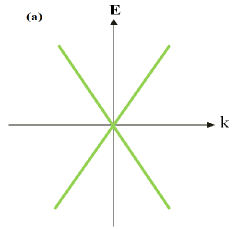
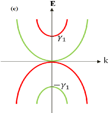
Figure 3: Energy bands of monolayer graphene (a), AA- stacked bilayer graphene (b) and AB-stacked bilayer graphene (c). In Figures (b) and (c), the green and red lines correspond to the lower $(c=-1)$ and upper $(c=1)$ layers, respectively.

The differential equation (18) offers straightforward solutions for $\Phi_{A}(r)$ in terms of the Bessel function, which is

$$\Phi_{A}(r)=C_{1}J_{m}(k_{h,+}r)+C_{2}J_{m}(k_{h,-}r)$$ (20)

where the sign $+$ ($c=+1$) and sign $-$ ($c=-1$) correspond to the upper and lower layer, respectively. While, the remains solutions can be obtained from (17) as

$$\Phi_{B}(r)=-h\left[C_{1}J_{m-1}(k_{h,+}r)+C_{2}J_{m-1}(k_{h,-}r)\right]$$

$$\Phi_{B^{\prime}}(r)=h\left[C_{1}J_{m-1}(k_{h,+}r)-C_{2}J_{m-1}(k_{h,-}r)\right]$$

$$\Phi_{A^{\prime}}(r)=-C_{1}J_{m}(k_{h,+}r)+C_{2}J_{m}(k_{h,-}r).$$ (21)

After obtaining the solution inside the quantum dot, it is natural to ask about the eigenvalues associated to the bound states of the system. To answer this inquiry we use the boundary conditions given in (16) to end up with

$$C_{1}\left[J_{m}(k_{h,+})-h\tau J_{m-1}(k_{h,+})\right]=C_{2}\left[J_{m}(k_{h,-})-h\tau J_{m-1}(k_{h,-})\right]$$ (22)

$$C_{1}\left[J_{m}(k_{h,+})+h\tau J_{m-1}(k_{h,+})\right]=-C_{2}\left[J_{m}(k_{h,-})+h\tau J_{m-1}(k_{h,-})\right].$$ (23)

These can be solved to obtain the following characteristic equation for the allowed eigenenergies $E$ of the quantum dot

$$\frac{J_{m}(k_{h,+})-h\tau J_{m-1}(k_{h,+})}{J_{m}(k_{h,+})+h\tau J_{m-1}(k_{h,+})}+\frac{J_{m}(k_{h,-})-h\tau J_{m-1}(k_{h,-})}{J_{m}(k_{h,-})+h\tau J_{m-1}(k_{h,-})}=0$$ (24)

which will be numerically analyzed as well as compared to those obtained for monolayer and AB-staked bilayer graphene systems.

3.2 Nonzero magnetic field

Now we consider our system in the presence of a perpendicular magnetic field and look for the solutions of the energy spectrum. To proceed, we choose the symmetric gauge $\vec{A}=\frac{B_{0}}{2}(0,r,0)$ to write the corresponding momentum operators $\pi$ and $\pi^{\dagger}$ as

$$\pi=v_{F}e^{i\theta}\left[-i\hbar(\frac{\partial}{\partial r}+\frac{i\partial}{r\partial\theta})+i\frac{eBr}{2}\right]$$ (25)

$$\pi^{\dagger}=v_{F}e^{-i\theta}\left[-i\hbar(\frac{\partial}{\partial r}-\frac{i\partial}{r\partial\theta})-i\frac{eBr}{2}\right].$$ (26)

Implementing these operators in the Hamiltonian (1) and acting on the four-component wave function $\Psi=e^{im\theta}\left[\Phi_{A},ie^{-i\theta}\Phi_{B},ie^{-i\theta}\Phi_{B^{\prime}},\Phi_{A^{\prime}}\right]^{T}$ to get the four coupled first-order differential equations

$$\left(\frac{\partial}{\partial r}-\frac{m-1}{r}-\beta r\right)\Phi_{B}(r)=E\Phi_{A}(r)-\gamma\Phi_{A^{\prime}}(r)$$ (27a)

$$\left(\frac{\partial}{\partial r}+\frac{m}{r}+\beta r\right)\Phi_{A}(r)=-E\Phi_{B}(r)+\gamma\Phi_{B^{\prime}}(r)$$ (27b)

$$\left(\frac{\partial}{\partial r}+\frac{m}{r}+\beta r\right)\Phi_{A^{\prime}}(r)=-E\Phi_{B^{\prime}}(r)+\gamma\Phi_{B}(r)$$ (27c)

$$\left(\frac{\partial}{\partial r}-\frac{m-1}{r}-\beta r\right)\Phi_{B^{\prime}}(r)=E\Phi_{A^{\prime}}(r)-\gamma\Phi_{A}(r).$$ (27d)

Decoupling the above equations with respect to $\Phi_{A}$ to obtain

$$\left[\frac{\partial^{2}}{\partial r^{2}}+\frac{1}{r}\frac{\partial}{\partial r}-\left(2\beta(m-1)+\frac{m^{2}}{r^{2}}+\beta^{2}r^{2}-k_{h,c}^{2}\right)\right]\Phi_{A}(r)=0$$ (28)

where $k_{h,c}$ is given in (19) and $\beta=\frac{eBR}{2\hbar}$. In order to solve the differential equation (28), we make the following ansatz

$$\Phi_{A}(r)=r^{|m|}e^{-\frac{r^{2}\beta}{2}}\chi(r^{2})$$ (29)

and define a new variable $\xi=\beta r^{2}$. Substituting (29) into (28) to get

$$\left[\xi\frac{\partial^{2}}{\partial{\xi}^{2}}+(b-\xi)\frac{\partial}{\partial\xi}-n_{h,c}\right]\chi(\xi)=0$$ (30)

where we have set the quantities

$$b=1+|m|,\qquad n_{h,c}=-\frac{k_{h,c}^{2}}{4\beta}+\frac{m+|m|}{2}.$$ (31)

(30) can be solved to get the following combination

$$\chi(\xi)=C_{1}\tilde{M}(n_{h,+},b,\xi)+C_{2}\tilde{M}(n_{h,-},b,\xi)$$ (32)

where the first term corresponds to the upper layer solution and the second one corresponds to the lower layer solution. $\tilde{M}(n,b,\xi)$ is the regularized confluent hypergeometric function, $C1$ and $C_{2}$ are normalization constants. From (29) and (32), we obtain the first spinor component

$$\Phi_{A}(r)=r^{|m|}e^{-\frac{\beta r^{2}}{2}}\left(C_{1}\tilde{M}(n_{h,+},b,\beta r^{2})+C_{2}\tilde{M}(n_{h,-},b,\beta r^{2})\right)$$ (33)

and the others come as

$$\Phi_{B}(r) = r^{|m|-1}e^{-\frac{\beta r^{2}}{2}}\left[\frac{C_{1}}{2(\gamma+E)}\left(r^{2}\eta_{+}\tilde{M}(n_{h,+},b+1,\beta r^{2})-\zeta\tilde{M}(n_{h,+},b,\beta r^{2})\right)\right.$$ (34)

$$\left.-\frac{C_{2}}{2(\gamma-E)}\left(r^{2}\eta_{-}\tilde{M}(n_{h,-},b+1,\beta r^{2})-\zeta\tilde{M}(n_{h,-},b,\beta r^{2})\right)\right]$$

$$\Phi_{B^{\prime}}(r) = -r^{|m|-1}e^{-\frac{\beta r^{2}}{2}}\left[\frac{C_{1}}{2(\gamma+E)}\left(r^{2}\eta_{+}\tilde{M}(n_{h,+},b+1,\beta r^{2})-\zeta\tilde{M}(n_{h,+},b,\beta r^{2})\right)\right.$$ (35)

$$\left.+\frac{C_{2}}{2(\gamma-E)}\left(r^{2}\eta_{-}\tilde{M}(n_{h,-},b+1,\beta r^{2})-\zeta\tilde{M}(n_{h,-},b,\beta r^{2})\right)\right]$$

$$\Phi_{A^{\prime}}(r) = -r^{|m|}e^{-\frac{\beta r^{2}}{2}}\left(C_{1}\tilde{M}(n_{h,+},b,\beta r^{2})-C_{2}\tilde{M}(n_{h,-},b,\beta r^{2})\right)$$ (36)

where the quantities are

$$\eta_{\pm}=2\beta(|m|-m+2)+(\gamma\pm E)^{2},\qquad\zeta=2(|m|+m+2\beta r^{2}).$$ (37)

To get the allowed energy for the quantum dots we use again the infinite-mass boundary condition given in (16). Doing this to get

$$C_{1}\left[\left(1-\frac{\tau\zeta}{2(\gamma+E)}\right)\tilde{M}(n_{h,+},b,\beta)+\frac{\tau\eta_{+}}{2(\gamma+E)}\tilde{M}(n_{h,+},b+1,\beta)\right]$$

$$=C_{2}\left[\left(1+\frac{\tau\zeta}{2(\gamma-E)}\right)\tilde{M}(n_{h,-},b,\beta)-\frac{\tau\eta_{-}}{2(\gamma-E)}\tilde{M}(n_{h,-},b+1,\beta)\right]$$ (38)

$$C_{1}\left[\left(1+\frac{\tau\zeta}{2(\gamma+E)}\right)\tilde{M}(n_{h,+},b,\beta)-\frac{\tau\eta_{+}}{2(\gamma+E)}\tilde{M}(n_{h,+},b+1,\beta)\right]$$

$$=-C_{2}\left[\left(1-\frac{\tau\zeta}{2(\gamma-E)}\right)\tilde{M}(n_{h,-},b,\beta)+\frac{\tau\eta_{-}}{2(\gamma-E)}\tilde{M}(n_{h,-},b+1,\beta)\right].$$ (39)

By the eliminating the constants $C_{1}$ and $C_{2}$, we finally find the characteristic equation for the allowed eigenenergies $E$ in the case of nonzero magnetic field. This is

$$\frac{(2(\gamma+E)-\tau\zeta)\tilde{M}(n_{h,+},b,\beta)+\tau\eta_{+}\tilde{M}(n_{h,+},b+1,\beta)}{(2(\gamma+E)+\tau\zeta)\tilde{M}(n_{h,+},b,\beta)-\tau\eta_{+}\tilde{M}(n_{h,+},b+1,\beta)}$$

$$+\frac{(2(\gamma-E)+\tau\zeta)\tilde{M}(n_{h,-},b,\beta)-\tau\eta_{-}\tilde{M}(n_{h,-},b+1,\beta)}{(2(\gamma-E)-\tau\zeta)\tilde{M}(n_{h,-},b,\beta)+\tau\eta_{-}\tilde{M}(n_{h,-},b+1,\beta)}=0.$$ (40)

After obtaining the infinite-mass boundary condition and the eigenenergies of the QD in the presence and absence of a perpendicular magnetic field, we numerically study the energy levels by using the above equations and underline the behavior of our system.

4 Results and discussion

Let us first discuss the energy spectrum in the absence of magnetic field by using equation (24). In discussing the properties of the energy spectrum, we use the notation $E^{q}(\tau,m)$, where $q\equiv e\ (h)$ denotes the electron (hole), $\tau$ is the valley index and it is equal to $+1$ ($-1$) for the $K$ ($K^{\prime}$) valley and $m$ correspond to the total angular quantum number. The fact that the Bessel functions obey the following properties

$$J_{n}(x)=(-1)^{n}J_{-n}(x),\qquad J_{n}(x)=(-1)^{n}J_{n}(-x)$$ (41)

we can derive interesting results. First, the intervalley spectrum symmetry is present, where the $m$ states in the $K$ valley have equal energies to the $-m+1$ states in the $K^{\prime}$ valley

$$E^{e,h}(\tau,m)=E^{e,h}(-\tau,-m+1)$$ (42)

Furthermore, there is a symmetry between the electron $m$ states and the hole $-m+1$ states

$$E^{e}(\tau,m)=-E^{h}(\tau,-m+1)$$ (43)

Also, we have another interesting symmetry indicate the intervalley electron-hole symmetry between the states of the same quantum number $m$

$$E^{e}(\tau,m)=-E^{h}(-\tau,m)$$ (44)

The intervalley electron-hole symmetry are also present in the case for AB-stacked bilayer graphene [19] with infinite-mass barrier. We note that our results are compatible with those obtained for monolayer graphene for infinite-mass boundary conditions [18].

In Figure 4, we plot the energy levels for a circular AA-stacked bilayer graphene QD as function of the dot radius $R$ for $m=\pm 1$ and $m=0$. The $K$ valley spectrum is depicted by the solid black lines, while the dashed blue lines denote the energy levels in the $K^{\prime}$ valley. One can see that the energy spectrum shows two set of levels. They are just the double copies of the energy spectrum corresponding to single layer graphene, one shifted up by $+\gamma$ and other one shifted down by $-\gamma$, where $\gamma=200\ meV$ is the interlayer coupling. We notice that the upper one corresponds to the upper layer and the lower one corresponds to the lower layer. For large $R$, the set of levels corresponding to the upper layer converges to the interlayer hopping energy $\gamma=200\ meV$. However, the set levels corresponding to the lower layer, converge to $-200\ meV$.

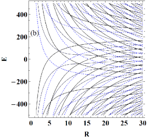
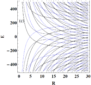
Figure 4: Energy spectrum of a circular AA-stacked bilayer graphene quantum dots as a function of the dot radius. (a) $m=-1$, (b) $m=0$ and (c) $m=1$. The energy states for the $K$ valley ($\tau=1$) are drown with dashed blue lines, those for the $K^{\prime}$ valley ($\tau=-1$) with solid black lines.

Now, we switch to the case with a nonzero magnetic field. In Figure 5, we plot the energy levels as function of the dot radius $R$ for $m=0,\ \pm 1$ and $B=5T$ for both valleys. From (3.2) we notice that the presence of the magnetic field breaks all symmetry properties except one

$$E^{e}(\tau,m)=-E^{h}(-\tau,m)$$ (45)

We clearly observe form Figures 4 and 5, the crossing between the levels of two different valleys for $E=0$. Also, as long as the size of the dot is increasing the energy spectrum becomes weakly dependent on the dot radius. In addition, we notice that this symmetry is obtained for monolayer [18] and AB-stacked bilayer graphene [19] in the presence of nonzero magnetic field with infinite-mass barrier.

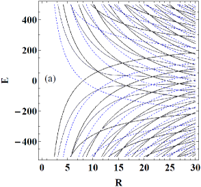
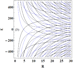
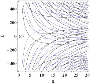
Figure 5: Energy spectrum of a circular AA-stacked bilayer graphene quantum dots as a function of the dot radius. (a) $m=-1$, (b) $m=0$ and (c) $m=1$ with $B=5\ T$. The energy states for the $K$ valley ($\tau=1$) are drown with dashed blue lines. Those for the $K^{\prime}$ valley ($\tau=-1$) with solid black lines.

Now we study the energy spectrum versus the magnetic field. In Figure 6, we show the energy levels of a circular quantum dot as a function of a perpendicular magnetic field for $R=50\ nm$ and $-2\leq m\leq 2$. The energy levels corresponding to the $K$ and $K^{\prime}$ valleys are shown, respectively, by the solid blue lines and dashed red lines. We can clearly see from Figures 5 that for zero magnetic field the energy states are not equidistant in contrast to the case of semiconductor QDs [29]. From Figure 6(a), we observe that for higher magnetic field the energy levels approach the Landau levels (LLs) of AA-stacked bilayer graphene. Moreover, the carrier confinement can be subdivided in two regimes. The first one is characterized by the weak magnetic field, where the confinement is due to the infinite-mass barrier. Whereas, the second regime is manifested at large magnetic field where the influence of the infinite-mass barrier is suppressed and the confinement becomes dominated by the magnetic field. We notice that the transition between these two confinement regimes takes place as the magnetic field increases. The transition points between the two regimes can be defined when the energies of the states in the dot differ negligibly from the LLs energy. It can be seen that the transition points shift toward larger magnetic field with lower $m$.

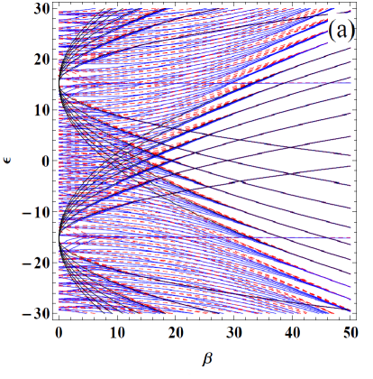
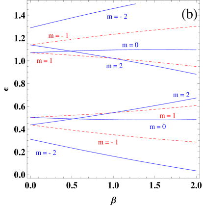
Figure 6: Energy spectrum of a circular AA-stacked bilayer graphene quantum dots as a function of a perpendicular magnetic field for $R=50\ nm$ and $-2\leq m\leq 2$. The energy states for the $K$ valley ($\tau=1$) are drown with solid blue lines, those for the $K^{\prime}$ valley ($\tau=-1$) with dashed red lines. The black solid lines correspond the Landau levels of AA-stacked bilayer graphene.

Figure 6(b) shows an enlargement of the low energy levels, corresponding to both valleys $K$ and $K^{\prime}$, at small magnetic field. From this we can see that, for zero magnetic field, the two degenerate states $E(1,m=2)$ and $E(-1,m=-1)$ belong to different valleys. Also, the others degenerate levels $E(1,m=0)$ and $E(-1,m=1)$ belong to different valleys. This result confirms the intervalley spectrum symmetry $E^{e,h}(\tau,m)=E^{e,h}(-\tau,-m+1)$. It may be noted that the application of a perpendicular magnetic field leads to the discretization of the energy spectrum. This can explain the fact that for nonzero magnetic field the degeneracy is broken.

In summary, we notice that the asymptotic behavior of the energy levels for both valleys $K$ and $K^{\prime}$ can be derived by using infinite-mass boundary conditions for large magnetic field. Doing this to end up with

$$E^{e,h}_{m,n}(\beta)=c\gamma\pm\sqrt{4\beta\left(n+\frac{m+|m|}{2}\right)}$$ (46)

where $c=\pm 1$ refer to the cone index, the sign $\pm$ accounts for the particle type (electron/hole) and the Landau levels index is denoted by $n$. Hence, we retrieve the well-known LLs for monolayer graphene from (46) for the limit $\gamma=0$. The first LL ($n=1$) is composed of $m\leq 0$ in both valleys $K$ and $K^{\prime}$. Similarly, the higher energy LLs ($n>1$) satisfy the condition $m\leq n$. This behavior is similar to that in monolayer [18] and AB-stacked bilayer graphene [19] with infinite-mass barrier and also for semiconductors [29].

5 Conclusion

In this paper, we considered a system of bilayer of graphene in the Bernal AA stacking and assumed that the carriers are confined in a circular areas of radius $R$, which was modeled by an infinite-mass barrier. From the eigenvalue equation, we derived the infinite-mass boundary condition in AA-stacked bilayer graphene quantum dot. This was only region I dependent, which means that the region outside the dot was forbidden for particles. The infinite-mass boundary condition allowed us to investigate the energy levels in the absence and presence of the magnetic field.

More precisely, after obtaining the corresponding wave functions inside and outside the quantum dot, we applied the obtained infinite-mass boundary conditions to find the energy levels of a circular graphene quantum dots for zero and nonzero magnetic field. The energy spectrum exhibited an intervalley spectrum symmetry ((42), (44)) and also an electron-hole symmetry (43). Furthermore, we found that the presence of a nonzero magnetic field broke all symmetry properties except one given in (44). The obtained energy spectrum symmetry are similar to those obtained in monolayer graphene for infinite-mass boundary conditions. However, the intervalley electron-hole symmetry is also present in the case of AB-stacked bilayer graphene.

Our results showed that the energy spectrum presents two sets of states as function of the quantum dot radius $R$. The upper set corresponds to the upper layer and the lower one corresponds the the lower layer. For large $R$, the upper set converges to the interlayer hopping energy $+\gamma$, whereas the lower set converges to $-\gamma$. In addition, we analyzed the magnetic field dependence of the energy spectrum. Indeed, for zero magnetic field, we found that the energy states are not equidistant in contrast to the results reported for semiconductor quantum dots. However, in the presence of a magnetic field we obtained two regimes of carriers confinement: for weak magnetic field the confinement is due to the infinite-mass barrier and for large magnetic field the influence of the infinite-mass barrier is suppressed, hence the confinement becomes dominated by magnetic field. Therefore, the transition between these two confinement regimes takes place as long as the magnetic field increases. By increasing the magnetic field, the energy levels of a circular quantum dot approach the Landau levels for AA-stacked bilayer graphene. Our results showed that the degenerate states, for zero magnetic field, belong to different valleys. For nonzero magnetic field, this degenerate was broken, owing to the discretization of the energy spectrum when a magnetic field is applied.

References

- [1] K. S. Novoselov, A. K. Geim, S. V. Morozov, D. Jiang, Y. Zhang, S. V. Dubonos, I. V. Grigorieva and A. A. Firsov, Science 306, 666 (2004).
- [2] K. S. Novoselov, D. Jiang, T. Booth, V. V. Khotkevich, S. M. Morozov and A. K. Geim, Proc. Natl Acad. Sci. 102, 10451 (2005).
- [3] A. H. Castro Neto, F. Guinea, N. M. R. Peres, K. S. Novoselov and A. K. Geim, Rev. Mod. Phys. 81, 1 (2009).
- [4] M. I. Katsnelson, K. S. Novoselov and A. K. Geim, Nat. Phys. 2, 620 (2006).
- [5] V. P. Gusynin and S. V. Sharapov, Phys. Rev. Lett. 95, 14 (2005).
- [6] G. W. Semenoff, Phys. Rev. Lett. 53, 2449 (1984).
- [7] D. P. DiVincenzo and E. J. Mele, Phys. Rev. B 29, 1685 (1984).
- [8] J. D. Bernal, Phys. Eng. Sci. 106, 749 (1924).
- [9] J. C. Charlier, X. Gonze and J. P. Michenaud, Phys. Rev. B 43, 6 (1991).
- [10] J.-K. Lee, S.-C. Lee, J.-P. Ahn, S.-C. Kim, J. I. B. Wilson and P. John, J. Chem. Phys. 129, 234709 (2008).
- [11] P. L. de Andres, R. Ramirez and J. A. Vergés, Phys. Rev. B 77, 045403 (2008).
- [12] T. Chakraborty Quantum Dots (Amsterdam: Elsevier) (1999).
- [13] P. G. Silvestrov and K. B. Efetov, Phys. Rev. Lett. 98, 016802 (2007).
- [14] A. Matulis and F. M. Peeters, Phys. Rev. B 77, 115423 (2008).
- [15] J. M. Pereira, V. Mlinar, F. M. Peeters and P. Vasilopoulos, Phys. Rev. B 74, 045424 (2006).
- [16] G. Giavaras, P. A. Maksym and M. Roy, J. Phys. Condens. Matt. 21, 102201 (2009).
- [17] P. Recher, J. Nilsson, G. Burkard and B. Trauzettel, Phys. Rev. B 79, 085407 (2009).
- [18] M. Grujić, M. Zarenia, A. Chaves, M. Tadić, G. A. Farias and F. M. Peeters, Phys. Rev. B 84, 205441 (2011).
- [19] D. R. da Costa, M. Zarenia, A. Chaves, G. A. Farias and F. M. Peeters, Carbon 78, 392 (2014).
- [20] M. Zarenia, A. Chaves, G. A. Farias and F. M. Peeters, Phys. Rev. B 84, 245403 (2011).
- [21] A. V. Rozhkov and F. Nori, Phys. Rev. B 81, 155401 (2010).
- [22] S. Schnez, K. Ensslin, M. Sigrist and T. Ihn, Phys. Rev. B 78, 195427 (2008).
- [23] C. J. Tabert and E. J. Nicol, Phys. Rev. B 86, 075439 (2012).
- [24] M. Ramezani, A. Matulis and F. M. Peeters, Phys. Rev. B 84, 245413 (2011).
- [25] D. S. L. Abergel, V. Apalkov, J. Berashevich, K. Ziegler and T. Chakraborty, Adv. Phys. 59, 261 (2010).
- [26] P. R. Wallace, Phys. Rev. B 71, 622 (1947).
- [27] B. Partoens and F. M. Peeters, Phys. Rev. B 74, 075404 (2006).
- [28] S. Schnez, K. Ensslin, M. Sigrist and T. Ihn, Phys. Rev. B 78, 195427 (2008)
- [29] C. S. Lent, Phys. Rev. B 43, 4179 (1991).