Kinetic Theory of Positron-Impact Ionization in Gases

Abstract

A kinetic theory model is developed for positron-impact ionization (PII) with neutral, rarefied gases. Particular attention is given to the sharing of available energy between the post-ionization constituents. A simple model for the energy-partition function that qualitatively captures the physics of high-energy and near-threshold ionization is developed for PII, with free parameters that can be used to fit the model to experimental data. By applying the model to the measurements of Kover and Laricchia Kover and Laricchia (1998) for positrons in H₂, the role of energy-partitioning in PII for positron thermalisation is studied. Although the overall thermalisation time is found to be relatively insensitive to the energy-partitioning, the mean energy profiles at certain times can differ by more than an order of magnitude for the various treatments of energy-parititioning. This can significantly impact the number and energy distribution of secondary electrons.

I Introduction

An understanding of the behavior of positrons in gases underpins many areas of technology and scientific research Murphy and Surko (1992); Greaves et al. (1994); Coleman (2002); Petrovic et al. (2013); Panov (2013). Of particular interest are applications to the medical imaging technique of Positron Emission Tomography (PET) Czernin and Phelps (2002). To optimize PET technologies and quantify the associated radiation damage requires a thorough understanding of the processes by which an energetic positron (and the secondary species) thermalise. It has been shown recently by Sanche and co-workers Sanche (2003, 2005, 2008, 2009) that the secondary electrons created via ionization can cause significant DNA damage. The number of secondary electrons ejected along the positron track is on the order of $10^{4}$ per MeV of primary radiation produced in water Abril et al. (2011); Cobut et al. (1997), so it is clear that particular attention needs to be paid to the ionization process.

Although there has been extensive research on electrons in gases, positrons remain significantly less well understood. Specific collisional processes are avilable to the positron which do not exist for electrons, e.g. annihilation with an electron and positronium formation Charlton and Humberston (2001); Kauppila et al. (1986). Although the impact from either a sufficiently energetic positron or electron can ionize a gas molecule, the ionization process differs in a crucial way; ionization by positron impact is a particle-conserving process with respect to positrons, while ionization by electron impact is non-particle-conserving with respect to electrons Loffhagen and Winkler (1996); Ness and Nolan (2000); Winkler et al. (2002); Grubert and Loffhagen (2014); Dujko et al. (2014). The two types of ionization will be referred to as ‘positron-impact ionization’ (PII) and ‘electron-impact ionization’ (EII) respectively. In the framework of kinetic theory, Ness Ness (1985) developed a collision operator for EII but no positron equivalent has yet been developed. Instead, previous investigations Suvakov et al. (2008); Marler et al. (2009); White and Robson (2009, 2011); Bankovic et al. (2012a, b) have generally treated positron ionization as a simple excitation process which effectively assumes that the scattered positron receives all of the available post-ionization energy, although Petrovic et al. (2014) has highlighted the effects of the secondary electron energy distribution.

In this paper, a PII equivalent of the EII collision operator of Ness is derived for the first time. Macroscopic transport coefficients, such as mean energy and flux drift velocity, are compared for a simple benchmark model using both a kinetic theory approach based on the Boltzmann equation, and Monte Carlo simulation. Particular attention is paid to the effect of energy-sharing between post-ionization constituents, and the influence that different energy-partitioning models have on transport. A basic energy-partitioning model that captures, at least qualitatively, the physics of high energy and near-threshold positron ionization is proposed, which can then be fitted to the rather limited experimental data that is available. The new kinetic theory model is used to investigate the transport of positrons in dilute H₂ gas using a recently-compiled complete set of cross sections Petrovic et al. (2013), and the proposed energy-partitioning model fitted to the experimental data of Kover and Laricchia Kover and Laricchia (1998).

II Theory

II.1 The kinetic equation and its multi-term solution

The fundamental equation describing a swarm of positrons moving through a dilute gaseous medium subject to an electric field, $\mathbf{E}$, is the Boltzmann kinetic equation for the phase-space distribution function $f\equiv f\left(\mathbf{r},\mathbf{v},t\right)$ White and Robson (2011):

$$\left(\frac{\partial}{\partial t}+\mathbf{v}\cdot\nabla+\frac{q\mathbf{E}}{m}\cdot\frac{\partial}{\partial\mathbf{v}}\right)f =-J\left(f\right),$$ (1)

where $t$ is the time, and $\mathbf{r}$, $\mathbf{v}$, $q$ and $m$ are the position, velocity, charge and mass of the positron respectively. The right hand side describes the effect of collisions on the distribution function at a fixed position and velocity. Essentially, the Boltzmann equation is an equation of continuity in phase-space Cercignani (1998). Solving equation (1) for the distribution function yields all relevant information about the system. Macroscopic transport properties including mean energy and drift velocity can then be found via averages over the ensemble as detailed in Section II.3. The purpose of this paper is to investigate the effect of ionization, so for simplicity we will consider only spatially-homogeneous situations.

If there is a single preferred direction in the system, e.g. due to an electric field in plane parallel geometry, then the angular dependence of the velocity component can be adequately described by an expansion in terms of Legendre polynomials Robson et al. (2002), i.e. if $f\left(\mathbf{v},t\right)\rightarrow f\left(v,\mu,t\right)$, where $\mu=\hat{\mathbf{v}}\cdot\mathbf{\hat{E}}$, then

$$f\left(\mathbf{v},t\right) =\sum_{l=0}^{\infty}f_{l}\left(v,t\right)P_{l}(\mu),$$ (2)

where $P_{l}$ is the $l$-th Legendre polynomial Abramowitz and Stegun (1972). Substituting the expansion (2) into equation (1) and equating the coefficients of Legendre polynomials results in the following coupled partial differential equations for the $f_{l}$ in energy-space,

$$\frac{\partial f_{l}}{\partial t} +\sum_{p=\pm 1}\Delta_{l}^{(p)}\frac{qE}{m}\left(U^{{}^{\frac{1}{2}}}\frac{\partial}{\partial U}+p\frac{\left(l+\frac{3p+1}{2}\right)}{2}U^{{}^{-\frac{1}{2}}}\right)f_{l+p}\begin{array}[t]{cc}=-J_{l}\left(f_{l}\right)&\left(l=0,1,2,\dots,\infty\right)\end{array},$$ (4)

where $U=\frac{1}{2}mv^{2}$, $J_{l}$ is the Legendre decomposition of the collision operator, and

$$\Delta_{l}^{(+1)} =\frac{(l+1)}{(2l+3)},$$

$$\Delta_{l}^{(-1)} =\frac{l}{(2l-1)}.$$

Equation (4) represents an infinite set of coupled partial differential equations for the expansion coefficients, $f_{l}$. In practice, one must truncate the series (2) at a sufficiently high index, $l=l_{\mathrm{max}}$. The history of charged particle transport in gases has been dominated by the ‘two-term approximation’ Huxley and Crompton (1974), i.e., where only the first two terms have been included. The assumption of quasi-isotropy necessary for the two-term approximation is violated in many situations, particularly when inelastic collisions are included White et al. (2002) or when higher order moments are probed Boyle et al. (2015). Such an assumption is not necessary in our formalism. Rather, $l_{\mathrm{max}}$ is treated as a free parameter to be increased until some convergence or accuracy criterion is met.

II.2 Collision operators in the multi-term representation

To solve equation (4) we require the collision operators for all of the relevant collisional processes, and their representations in terms of Legendre polynomials, $J_{l}$. If we assume that the neutral background gas is at rest and in thermal equilibrium at a temperature $T_{0}$, then the background medium has a Maxwellian distribution in velocity space and the collision operator is linear in the swarm approximation Robson (2006). Below we detail the specific kinetic theory forms of the collision operator for conservative elastic and inelastic collisions, particle-loss collisions such as annihilation and positronium formation, and ionization, which is the focus of this work. A further expansion of each collision integral with respect to the ratio of swarm particle mass to neutral particle mass, $m/m_{0}$, has been performed. Because this ratio is small for positrons (and electrons), only the leading term of this expansion for each collision process and in each equation of the system (4) was taken into account.

The total collision operator can then be separated for each of the different types of processes, eg.

$$J =J^{\mathrm{el}}+J^{\mathrm{in}}+J^{\mathrm{ann}}+J^{\mathrm{Ps}}+J^{\mathrm{ion}},$$

where the right hand side terms represent the elastic, inelastic, annihilation, positronium formation and ionization collision operators respectively. Microscopic scattering information is included via the appropriate scattering cross sections Goldstein et al. (2001); Kauppila et al. (1985). It is more natural to work with the collision frequency rather than the scattering cross sections directly. A collision frequency, $\nu$, is defined for a particular process by

$$\nu(U) \equiv n_{0}\sqrt{\frac{2}{m}}U^{\frac{1}{2}}\sigma(U),$$ (5)

where $\sigma$ is the corresponding cross section of the process.

II.2.1 Conservative elastic and inelastic collisions

For particle-conserving elastic and inelastic collisions we assume the Wang-Chang et al. Wang-Chang et al. (1964) semi-classical collision operator and its limiting cases. For an elastic collision, if all terms proportional to the mass ratio are neglected there is no energy transfer during a collision. To obtain a non-zero expression, a first-order mass ratio approximation is required Davydov (1935), i.e.

$$J_{l}^{\mathrm{el}}\left(f_{l}\right)=\begin{cases}-\frac{2m}{m_{0}}U^{-\frac{1}{2}}\frac{\partial}{\partial U}\left[U^{\frac{3}{2}}\nu_{1}^{\mathrm{el}}(U)\left(f_{0}+kT_{0}\frac{\partial f_{0}}{\partial U}\right)\right]&l=0,\\ \nu_{l}^{\mathrm{el}}(U)f_{l}&l\geq 1,\end{cases}$$

where $\nu_{l}^{\mathrm{el}}=n_{0}\sqrt{\frac{2}{m}}U^{\frac{1}{2}}\left(\sigma_{0}^{\mathrm{el}}-\sigma_{l}^{\mathrm{el}}\right)$, and $\sigma_{l}$ is defined from the differential scattering cross section Goldstein et al. (2001), $\sigma(U,\mu)$, via,

$$\sigma_{l}\left(U\right)=2\pi\int_{0}^{\pi}d\mu P_{l}\left(\mu\right)\sigma(U,\mu).$$

If the background gas has internal degrees of freedom then, to zeroth order in the mass ratio, energy exchange can still occur through excitation and de-excitation of those internal states. Hence, unlike the isotropic part of the elastic collision integral, the scalar part of the inelastic collision integral does not vanish under a zeroth order mass assumption. The Legendre decomposed form of the inelastic collision operator in the cold gas limit is given by Frost and Phelps (1962); Holstein (1946)

$$J_{l}^{\mathrm{in}}\left(f_{l}\right) =\sum_{j}\nu_{j}^{\mathrm{in}}\left(U\right)f_{l}-\begin{cases}\begin{array}[]{c}\left(\frac{U+U_{j}}{U}\right)^{\frac{1}{2}}\nu_{j}^{\mathrm{in}}\left(U+U_{j}\right)f_{l}\left(U+U_{j}\right)\\ 0\end{array}&\begin{array}[]{c}l=0,\\ l\geq 1,\end{array}\end{cases}$$ (6)

where the subscript $j$ denotes the available inelastic channels, such as excitations and rotations, with an associated inelastic scattering cross section $\sigma_{j}^{\mathrm{in}}(U)$, and a threshold energy $U_{j}$. It is implicit in the above equation that there is no thermal excitation of internal states.

II.2.2 Annihilation and positronium formation

Positron annihilation and positronium formation occur through distinctly different physical mechanisms. However, from a transport theory perspective they each represent a unidirectional particle loss process, and hence the form of their collision operators are identical. Since there is no post-collision scattering the collision operator is simply Ness and Robson (1986),

$$J_{l}^{\mathrm{loss}}\left(f_{l}\right) =\sum_{k}\nu_{k}^{\mathrm{loss}}(U)f_{l},$$

where $k$ are the available loss process channels, and $\nu_{k}^{\mathrm{loss}}$ is the collision frequency for the $k$th loss process corresponding to the cross section $\sigma_{k}^{\mathrm{loss}}(U)$.

II.2.3 Ionization

Ionization by electron impact is fundamentally different from ionization by positron impact. Since the ejected electron is of the same species as the impacting particle, EII is a non-particle-conserving process, i.e., the indistinguishability of electrons leads to a gain in the number of electrons in the swarm. Since the scattered positron can be distinguished from the ejected electron, PII is a particle-conserving process. A different collision operator needs to be used for each case. In previous studies, PII was treated as a simple excitation process, which ignores the possible partitioning of energy between the scattered positron and ejected electron. In what follows, we develop an explicit expression for the PII operator.

Following the approach of Ness (1985), the details of which are given in Appendix A, the PII collision operator takes the form

$$J_{l}^{\mathrm{ion}}\left(f_{l}\right) =\nu^{\mathrm{ion}}\left(U\right)f_{l}\left(U\right)-\begin{cases}\begin{array}[]{c}{\displaystyle\int}\left(\frac{U^{\prime}}{U}\right)^{{}^{\frac{1}{2}}}P(U,U^{\prime})\nu^{\mathrm{ion}}\left(U^{\prime}\right)f_{0}(U^{\prime})dU^{\prime}\\ 0\end{array}&\begin{array}[]{c}l=0,\\ l\geq 1,\end{array}\end{cases}$$ (7)

where $U^{\prime}$ is the impact particle energy, and $\nu^{\mathrm{ion}}$ is the collision frequency for ionization, corresponding to an ionization cross section. The $P(U,U^{\prime})$ term is the energy-partitioning function, defined such that $P(U,U^{\prime})dU$ represents the probability of the positron having an energy in the range $U+dU$ for an incident positron of energy $U^{\prime}$. The energy-partitioning function has the following properties:

$$P(U,U^{\prime}) =\begin{array}[]{cc}0\ \mbox{for}&U^{\prime}<U+U_{I},\end{array}$$

$$\int_{0}^{U^{\prime}-U_{I}}\negthickspace P(U,U^{\prime})dU =\begin{array}[]{cc}1\ \mbox{for}&U^{\prime}\geq U+U_{I},\end{array}$$

where $U_{I}$ is the ionization threshold energy, i.e., the energy needed to overcome the electron binding. The energy-sharing, which is determined by the energy-partitioning function $P$, is a major theme in the present work. It will be shown in Section IV that different energy-partition models significantly affect positron transport.

II.3 Transport properties

The cross sections and collision operator terms represent the microscopic picture of positron interactions with the medium. The macroscopic picture, e.g. transport properties that represent experimental measurables, are obtained as averages of certain quantities with respect to the distribution function, $f$. Among the transport properties of interest in the current manuscript are the number density, $n$, flux drift velocity, $W$, and mean energy, $\epsilon$, of the positron swarm, which can be calculated via Robson (2006)

$$n =2\pi\left(\frac{2}{m}\right)^{\frac{3}{2}}\int dU\ U^{\frac{1}{2}}f_{0}(U),$$

$$W =\frac{1}{n}\frac{2\pi}{3}\left(\frac{2}{m}\right)^{2}\int dU\ Uf_{1}(U),$$

$$\epsilon =\frac{1}{n}2\pi\left(\frac{2}{m}\right)^{\frac{3}{2}}\int dU\ U^{\frac{3}{2}}f_{0}(U).$$

The focus of this paper is the ionization process, so it is also useful to calculate the average ionization collision rate defined by

$$\alpha^{\mathrm{ion}} =\frac{1}{n}2\pi\left(\frac{2}{m}\right)^{2}\int dU\ U^{\frac{1}{2}}\nu^{\mathrm{ion}}(U)f_{0}(U).$$

III The numerical approach for a multi-term solution

In this section we detail a numerical solution of the system of coupled ordinary differential equations, (4), once an $l$-index truncation has been applied.

III.1 Method of lines

The Method of Lines (MOL) Shampine (2005); Sadiku and Obiozor (2000) is a technique for solving PDEs in which all but one dimension is discretized. In developing a numerical solution to the Boltzmann equation, we choose to first discretize the energy- (or equivalently, speed-) space. In general, applying the MOL to linear PDEs results in a system of equations of the form

$$\mathbf{M}\frac{d}{dt}\mathbf{u} =\mathbf{L}\mathbf{u},$$ (8)

where $\left[u\right]_{i}=u_{i}(t)\equiv u(x_{i},t),$ and $\mathbf{L}$ and $\mathbf{M}$ are matrices resulting from the discretization process, commonly known as the “Stiffness Matrix” and “Mass Matrix” respectively Carver and Hinds (1978). The formerly continuous variable $x$ has been discretized into a set of $x_{i}$ for $i=0,1,...,n.$ The MOL formalism allows easy implementation of linear boundary conditions or constraints via the mass matrix. Let the discretized boundary conditions and constraints of (8) be represented by $\mathbf{G}\mathbf{u}=\mathbf{0}$, where $\mathbf{G}$ is a matrix and $\mathbf{0}$ represents a vector of zeros. Then clearly $\frac{d}{dt}\mathbf{G}\mathbf{u}=\mathbf{G}\frac{d}{dt}\mathbf{u}=\mathbf{0}$ and, provided the initial solution satisfies the constraints,

$$\mathbf{\overline{M}}\frac{d}{dt}\mathbf{u} =\overline{\mathbf{L}}\mathbf{u},$$ (9)

where $\mathbf{\overline{M}}$ and $\overline{\mathbf{L}}$ are the modified mass and stiffness matrices,

$$\mathbf{\overline{M}}=\left[\begin{array}[]{c}\mathbf{G}\\ \mathbf{M}\end{array}\right] ,\;\overline{\mathbf{L}}=\left[\begin{array}[]{c}\mathbf{0}\\ \mathbf{L}\end{array}\right].$$

In a pure MOL approach, the system of ODEs, (9), are solved analytically. However, one is eventually forced to discretize the time variable as well for complicated systems of equations, such as those arising from the discretization of the Boltzmann equation. In this work we choose to discretize the time dimension with a first-order implicit Euler method Butcher (2003), for its good stability properties. Applying the implicit Euler method to equation (8) or (9) gives

$$\left(\mathbf{M}-h\mathbf{L}\right)\mathbf{u}^{n+1} =\mathbf{M}\mathbf{u}^{n}$$ (10)

where $\mathbf{u}^{n}$ and $\mathbf{u}^{n+1}$ are the solution vector, $\mathbf{u}$, at times $t_{n}$ and $t_{n+1}$, and $h=t_{n+1}-t_{n}$ is the time step. For linear systems, equation (10) can be solved directly with linear algebra techniques.

III.2 Finite difference representation in energy-space

The finite difference method Burden and Faires (1993) is a local approximation method which seeks to replace the continuous derivatives by a weighted difference-quotient of neighboring points. It is widely used, simple to program, and leads to sparse matrices with band structures approximating derivatives LeVeque (2007). Similar to the work of Winkler and collaborators Winkler et al. (1984); Loffhagen and Winkler (1996); Leyh et al. (1998), the system of ODEs is discretized at centered points using a centered difference scheme, i.e.,

$$\left.\frac{df(U,t)}{dx}\right|_{U_{i+1/2}} =\frac{f(U_{i+1},t)-f(U_{i},t)}{U_{i+1}-U_{i}},$$

$$f(U_{i+1/2},t) =\frac{f(U_{i+1})+f(U_{i})}{2}.$$

Although a general form can be constructed for an arbitrary grid, the simplest case is for evenly spaced points, i.e.

$$U_{i}=i\Delta U\ \ 0\leq i\leq n,$$

where $\Delta U$ is a constant. Discretizing at the center between two solution nodes results in a system of linear equations that is underdetermined. The extra information is naturally provided by boundary conditions which are appended to the system.

III.3 Initial and boundary conditions

In positron experiments Charlton and Humberston (2001), unmoderated positrons have a peak in their emission energy spectrum of around half an MeV, which then lose energy rapidly via collisions. There is little information about the initial source distribution in thermalisation experiments Campeanu and Humberson (1977). For our purposes, we wish to probe the influence of PII collisions, and accordingly choose an initial distribution with a mean energy far above the ionization threshold so that a large range of the ionization cross section can be sampled during relaxation. One of the source distributions used by Campeanu and Humberston Campeanu and Humberson (1977) in their investigations of helium is a distribution that is constant in speed space up to some sufficiently high cut-off value, $v_{\mathrm{max}}=\sqrt{2U_{max}/m}$, i.e. $f_{0}(v)=\Theta\left(v_{\mathrm{max}}-v\right)C$, where $\Theta(x)$ is the Heaviside step function. The mean energy of this distribution function is given by $\epsilon=\frac{3}{5}U_{\mathrm{max}}$. We will use this type of initial distribution for our investigations of thermalisation and shall choose $U_{\mathrm{max}}$ to be sufficiently high to sample the ionization cross sections accordingly.

The system of coupled equations (4) requires boundary conditions on the expansion coefficients $f_{l}$. Winkler and collaborators Winkler et al. (1984); Loffhagen and Winkler (1996); Leyh et al. (1998) have analyzed the multi-term, even-order approximation, and discovered that the general solution of the steady-state hierarchy contains $\tfrac{1}{2}\left(l_{\mathrm{max}}+1\right)$ non-singular and $\tfrac{1}{2}\left(l_{\mathrm{max}}+1\right)$ singular fundamental solutions when $U$ approaches infinity, and the physically relevant solution has to be sought within the non-singular part. They give the boundary conditions necessary for the determination of the non-singular physically relevant solution as

$$f_{l}(U=0) =\begin{array}[]{cc}0&\mbox{for odd $l$},\end{array}$$

$$f_{l}(U=U_{\infty}) =\begin{array}[]{cc}0&\mbox{for even $l$},\end{array}$$

$$f_{l}(U>U_{\infty}) =\begin{array}[]{cc}0&\mbox{for all $l$},\end{array}$$

where $U_{\infty}$ represents a sufficiently large energy. In practice, $U_{\infty}$ has to be determined in a prior calculation, and is chosen such that the value of $f_{0}(U_{\infty})$ is less than $10^{-10}$ of the maximum value of $f_{0}$.

IV Results and discussion

In this section we will apply both the kinetic theory technique detailed in the previous sections, and a Monte Carlo simulation Tattersall et al. (2015), to describe positron transport in a benchmark model, and positron transport in real $H_{2}$ gas. Comparisons are made to EII where possible. Particular attention is given to the role of energy-partitioning between the scattered and ejected particles post-ionization, and a simple energy-partitioning model is proposed to capture the underlying physics.

IV.1 Positron ionization benchmarking

We first discuss several benchmark models for EII which can act as a test bed for our numerical techniques and solution model. The Lucas-Saelee Lucas and Saelee (1975) model is a popular benchmark, but focuses on the differences between excitation and ionization rather than energy-partitioning specifically. Taniguchi et al. Taniguchi et al. (1977) modified the partition function of the Lucas-Saelee model, which assumes a distribution with all energy-sharing fractions equiprobable, to instead share energy equally between the two electrons, but found that it did not alter the transport coefficients significantly. Instead, Ness and Robson Ness and Robson (1986) proposed a step model for testing energy-sharing for EII, which was shown to have some variation for the partitionings they investigated. The details of the model are:

$$\sigma_{0}^{\mathrm{el}}-\sigma_{l}^{\mathrm{el}} =10\ \mbox{\AA}^{2},$$ (11)

$$\sigma^{\mathrm{in}} =\begin{cases}\begin{array}[]{c}1\ \mbox{$\text{\AA}^{2}$}\\ 0\end{array}&\begin{array}[]{c}U\geq 10\ \mbox{eV},\\ U<10\ \mbox{eV},\end{array}\end{cases}$$

$$\sigma^{\mathrm{ion}} =\begin{cases}\begin{array}[]{c}1\ \mbox{\AA}^{2}\\ 0\end{array}&\begin{array}[]{c}U\geq 15\ \mbox{eV},\\ U<15\ \mbox{eV},\end{array}\end{cases}$$

$$m_{0} =25\ \mbox{amu},$$

$$T_{0} =0\ \mbox{K}.$$

Transport coefficients for EII calculated using kinetic theory are compared against the results of Ness and Robson, and the Monte Carlo simulations in Table 4 of Appendix B. The results support the integrity of our methods and solutions. Transport coefficients for PII under this model are given in Table 1 for varying energy sharing fractions, $Q$, where $Q=\frac{U}{U^{\prime}-U_{I}}$. As described in Appendix A the collision operator (7) breaks down when $Q=0$, hence there is no value given in Table 1 corresponding to the kinetic model for positrons with $Q=0$. No previous positron impact calculations exist for model (11), so the transport properties from our kinetic theory model are compared solely against an independent Monte Carlo simulation in Table 1. The uncertainty in the Monte Carlo simulations has been estimated to be less than $1\%$ for the ionization collision rates, and less than $0.5\%$ (generally less than $0.3\%$) for the drift velocity and mean energy. The two approaches give $\alpha^{\mathrm{ion}}/n_{0}$, $\epsilon$ and $W$ values which differ by less than $0.6\%$, $0.3\%$ and $0.3\%$ respectively, over the range of reduced electric fields and available energy fractions, all of which are within the corresponding Monte Carlo uncertainty.

As the reduced field, $E/n_{0}$, is increased, the velocity distribution function samples more of the ionization process leading to a greater ionization rate and a stronger dependence of the transport coefficients on the post-collision energy partitioning as shown in Table 1.

Table 1: Comparison of average ionization rates, $\alpha^{\mathrm{ion}}/n_{0}$, mean energies, $\epsilon$, and flux drift velocities, $W$, for PII for model (11) for different reduced fields $E/n_{0}$ and energy sharing fractions $Q$. Columns ‘Current’ correspond to the current kinetic theory calculations, and columns ‘MC’ are the results of the Monte Carlo simulation. Note, $Q=\mathrm{AFE}$ corresponds to “all fractions equiprobable”.

$E/n_{0}$		$\alpha^{\mathrm{ion}}/n_{0}$		$\epsilon$		$W$
(Td)	$Q$	($10^{-15}$m3s-1)		(eV)		($10^{5}$ms-1)
		Current	MC	Current	MC	Current	MC
$300$	$0$		1.711		6.869		2.767
	$1/4$	1.720	1.718	6.919	6.931	2.722	2.730
	$1/3$	1.725	1.719	6.940	6.942	2.711	2.706
	$1/2$	1.740	1.739	6.983	6.979	2.693	2.689
	$2/3$	1.757	1.761	7.021	7.023	2.677	2.676
	$3/4$	1.767	1.774	7.041	7.040	2.671	2.664
	$1$	1.807	1.804	7.098	7.087	2.654	2.648
	AFE	1.745	1.739	6.979	6.981	2.699	2.701
$500$	$0$		4.856		9.210		3.951
	$1/4$	4.915	4.917	9.379	9.375	3.819	3.822
	$1/3$	4.955	4.949	9.446	9.450	3.789	3.780
	$1/2$	5.060	5.055	9.579	9.588	3.738	3.739
	$2/3$	5.211	5.208	9.716	9.714	3.697	3.697
	$3/4$	5.288	5.293	9.788	9.789	3.678	3.678
	$1$	5.565	5.599	10.03	10.05	3.627	3.628
	AFE	5.119	5.107	9.589	9.577	3.754	3.755
$800$	$0$		9.903		13.30		5.260
	$1/4$	10.21	10.23	13.75	13.76	4.986	4.992
	$1/3$	10.39	10.40	13.93	13.93	4.922	4.925
	$1/2$	10.84	10.83	14.32	14.33	4.816	4.818
	$2/3$	11.40	11.41	14.79	14.81	4.719	4.725
	$3/4$	11.68	11.70	15.07	15.09	4.672	4.678
	$1$	12.92	12.95	16.27	16.31	4.518	4.527
	AFE	10.92	10.94	14.38	14.36	4.850	4.857

The convergence of transport coefficients for $1000$ Td with increasing $l_{\mathrm{max}}$ is shown in Table 2. Since an even-order approximation is required for the appropriate boundary conditions, the $l_{\mathrm{max}}$ are odd in our calculations. Clearly the two-term approximation ($l_{\mathrm{max}}=1$) leads to an over-estimation of the ionization rate, mean energy and flux drift velocity by approximately $2\%$. Indeed six terms are required to achieve convergence to four significant figures.

Table 2: Convergence of transport properties with $l_{\mathrm{max}}$ for PII model (11) at $1000$ Td and $Q=1/2$.

	$\alpha^{\mathrm{ion}}/n_{0}$	$\epsilon$	$W$
$l_{\mathrm{max}}$	($10^{-15}$m3s-1)	(eV)	($10^{5}$ms-1)
$1$	12.77	18.23	5.460
$3$	12.47	17.96	5.350
$5$	12.48	17.95	5.349
$7$	12.48	17.95	5.349

The variation of mean energy with $Q$ for PII at a reduced electric field of $800$ Td is shown in Figure 1. For PII, the mean energy of the positron swarm increases monotonically with the energy-sharing fraction, $Q$. This behavior is to be expected, as the ejected electron directly removes energy from the positron swarm. The ionization collision frequency increases with energy in model (11), so that the greater the energy of the swarm, the higher the rate of ionization collisions. Hence $\alpha^{\mathrm{ion}}/n_{0}$ also increases monotonically with $Q$. The flux drift velocity, $W$ in contrast, decreases with increasing $Q$. The effect of collisions is to randomize the directions of the swarm particles, such that an increase in the ionization rate decreases the average velocity of the swarm. The transport properties for the ‘all fractions equiprobable’ (AFE) distribution are very similar to that of the equal-energy sharing case.

The variation of mean energy with $Q$ for EII at $800$ Td is shown in Figure 2. The mean energy profile is symmetrical about $Q=0.5$ due to the indistinguishability of post-collision electrons, and for $800$ Td has a concave shape with a minimum value corresponding to equal energy-sharing. It should be noted that, in contrast to PII where the mean energy always increases with $Q$, the exact nature of the EII mean energy profile depends on how the distribution function samples the elastic, inelastic and ionization cross sections. The variation in the transport properties for EII with respect to $Q$ for the fields considered is small, suggesting that EII is relatively insensitive to the exact nature of the energy-partitioning for the model (11). Ness and Makabe Ness and Makabe (2000) have shown that for EII in argon the choice of energy-sharing fraction can in fact cause differences of $\sim 25\%$, so that care must still be taken when choosing the energy-partitioning function.

The qualitative shape of the $Q$-dependence of the mean energy for PII is insensitive to the reduced electric field, and the range of values for a particular reduced field is considerably larger than that for EII. In previous positron studies Loffhagen and Winkler (1996); Winkler et al. (2002); Trunec et al. (2006); White and Robson (2009), PII has been treated as a standard excitation process. The current results suggest that PII is particularly sensitive to the form of the energy-partitioning and, if real-world PII differs significantly from the model of pure scattering with excitation, large errors can result. To comment on this, we need to develop a realistic model of PII energy-partitioning.

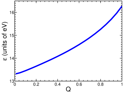
Figure 1: Variation of mean energy, $\epsilon$, with energy sharing fraction, $Q$, for PII model (11) at a reduced field of 800 Td.

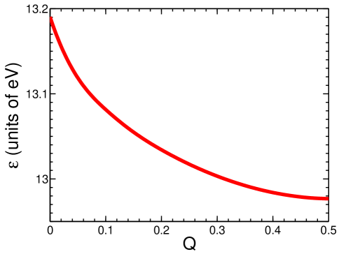
Figure 2: Variation of mean energy, $\epsilon$, with energy sharing fraction, $Q$, for EII model (11)at a reduced field of 800 Td.

IV.2 Positron ionization energy-partitioning model

We now wish to develop a model for post-ionization energy-partitioning that captures the following basic physical behaviors:

1. For high impact energies, the positron ionization scattering cross section approaches the electron ionization scattering cross section. The first Born approximation Brauner and Briggs (1986) is valid for high impact energies and shows a heavy bias towards the case where the scattered positron leaves the collision with almost all of the energy which is available post-collision.

2. For impact energies near the ionization threshold, there is significant correlation between the scattered positron and ejected electron. In the Wannier theory Wannier (1953) originally developed for near-threshold EII, the repulsion between the two electrons cause them to emerge with similar energies but in opposite directions. In terms of the interaction potential between the two electrons, one may talk about a Wannier ‘ridge’ upon which the system is in an unstable equilibrium. Klar Klar (1981) was the first to adapt Wannier’s classical idea to PII. As in Wannier’s theory the energy is predicted to be shared equally, however now the positron and electron emerge in similar directions due to the Coulomb attraction. Ashley et al. Ashley et al. (1996) measured the positron ionization cross-section in helium which they were able to accurately represent by a power law, albeit different to that derived by Klar. Ihra et al. Ihra et al. (1997) extended the Wannier theory to be consistent with both Klar and experiment. The success of these power law models justifies the assumption of equal energy-sharing at near-threshold impact energies, although recent experiments Arcidiacono et al. (2005) suggest a slight asymmetry. It should be noted that the positron and electron escape in similar directions with similar energies and are highly correlated, so no clear distinction between ionization and continuum state positronium can be made Charlton and Humberston (2001).

3. Ionization at intermediate energies appears to be a combination of the above two effects, i.e. a strong peak in the energy-sharing distribution corresponding to the scattered positron leaving with all the available energy, and a second peak occurring when the positron and electron emerge with similar energy and direction and in a highly correlated state. This feature has been shown in the studies of atomic hydrogen by Brauner et al. Brauner et al. (1989) and measured experimentally in H₂ by Laricchia and co-workers Kover and Laricchia (1998); Arcidiacono et al. (2005).

To capture simply the above three characteristics we propose a model consisting of an exponentially decaying function, $g_{\mathrm{high}}(Q)$, to represent the high impact energy ionization, and a rational polynomial (sometimes called the Cauchy or Lorentz distribution), $g_{\mathrm{low}}(Q)$ centered around equal energy-sharing to represent the near-threshold ionization i.e.,

$$g_{\mathrm{high}}(Q) =A_{\mathrm{high}}\exp(\beta_{\mathrm{high}}Q),$$ (12)

$$g_{\mathrm{low}}(Q) =A_{\mathrm{low}}\left[\beta_{\mathrm{low}}^{2}+\left(Q-0.5\right)^{2}\right]^{-1},$$ (13)

where $Q$ is the fraction of the available energy, $A_{\mathrm{high}}$ and $A_{\mathrm{low}}$ are normalization constants, and $\beta_{\mathrm{high}}$ and $\beta_{\mathrm{low}}$ are free parameters to be fitted. An energy-fraction-partitioning function which depends only on the impact energy and $Q$ can then be constructed as

$$g(U^{\prime},Q) =w(U^{\prime})g_{\mathrm{high}}(Q)+\left(1-w(U^{\prime})\right)g_{\mathrm{low}}(Q),$$ (14)

where $w(U^{\prime})$ is chosen as a hyperbolic tan function to transition smoothly between $g_{\mathrm{high}}$ and $g_{\mathrm{low}}$, i.e.,

$$w(U^{\prime}) =\frac{1}{2}\left[1+\tanh\left(\gamma\frac{U^{\prime}-U_{I}}{q}-\delta\right)\right],$$ (15)

where $q$ is the elementary charge, and $\gamma$ and $\delta$ are free parameters that control where and how sharp the transition is. The relationship between energy-fraction-partitioning function, $g(U^{\prime},Q)$, and the energy-partitioning function, $P(U,U^{\prime})$, used in equations (7) and (24) is given simply by

$$g(U^{\prime},Q)Q=P(U,U^{\prime})U.$$

In the following subsections we shall investigate a test model with reasonable values for the free parameters which can serve as a future benchmark model, and then fit the energy-partitioning model to real experimental H₂ data.

IV.2.1 Test model

In this subsection we investigate the effect that the energy-partitioning model (12)-(15) has on positron transport for a range of reduced electric field strengths. The parameters for the energy-partitioning function are

$$\beta_{\mathrm{high}} =10,$$

$$\beta_{\mathrm{low}} =0.05,$$ (16)

$$\gamma =0.05,$$

$$\delta =3.5,$$

with the same cross sections, neutral temperature and mass as the model (11). The energy-partition function for model (16) is displayed in Figure 3.

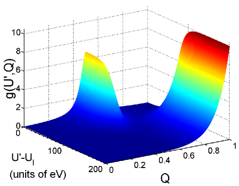
Figure 3: Variation of the energy-fraction-partition function with impact energy, relative to the ionization threshold, and energy sharing fraction, $Q$, for parameters (16)

Transport properties calculated via kinetic theory and Monte Carlo are shown in Table 3. The kinetic theory and Monte Carlo results agree to within $0.4\%$. Also included in the table for $800$ Td and $5000$ Td are the swarm properties assuming the energy-partitioning was replaced by only $g_{\mathrm{low}}$ or $g_{\mathrm{high}}$ respectively. At $800$ Td, the swarm properties for the full energy-partitioning model are close to that which results from the inclusion of only $g_{\mathrm{low}}$, which indicates that the distribution is generally sampling the even energy-sharing part of the full energy-partitioning distribution. At the higher field of $4000$ Td the swarm properties are now close to those that come from allowing only $g_{\mathrm{high}}$ to have an effect. As the field has increased, the distribution has shifted from sampling mostly the even sharing region, to the region that is heavily biased towards the positron getting large amounts of available energy.

Table 3: Comparison of average ionization rate, $\alpha^{\mathrm{ion}}/n_{0}$, mean energies, $\epsilon$, and flux drift velocities, $W$, for PII for model (16). The superscripts $a$ and $b$ refer to $w(U)=0$ and $w(U)=1$ respectively. Columns “Current” correspond to the current kinetic theory calculations, and columns “MC” are the results of Monte Carlo simulation.

$E/n_{0}$	$\alpha^{\mathrm{ion}}/n_{0}$		$\epsilon$		$W$
(Td)	($10^{-15}$m3s-1)		(eV)		($10^{5}$ms-1)
	Current	MC	Current	MC	Current	MC
$800$	10.92	10.90	14.40	14.37	4.810	4.814
$800^{a}$	10.86	10.85	14.35	14.32	4.816	4.820
$800^{b}$	12.48	12.37	15.82	15.70	4.555	4.585
$1600$	26.29	26.26	34.12	34.04	6.331	6.348
$2400$	40.97	40.88	65.56	65.42	6.910	6.932
$3200$	53.97	53.85	104.1	103.9	7.201	7.229
$4000$	64.95	64.90	144.8	145.0	7.491	7.517
$4000^{a}$	49.18	49.11	86.49	86.52	9.509	9.527
$4000^{b}$	66.96	66.64	149.5	149.2	7.150	7.178

IV.2.2 Model for positron-impact ionization in H₂

Laricchia and co-workers Kover and Laricchia (1998); Arcidiacono et al. (2005) have measured experimentally the energy-sharing of post-ionization species for PII for a specific impact energy and angle. Their results for ionization by a $100$ eV positron, where both the positron and electron emerge at the same angle of $0$ degrees, are included in Figure 4. It is evident that there is a bias towards the positron getting all or large amounts of the available energy, with a secondary peak close to equal energy-sharing due to electron-positron correlation effects. Our model predicts that this peak should occur at exactly $Q=0.5$, but experiments show that there is a slight energy-sharing asymmetry in positron ionization, such that the peak actually occurs at $Q>0.5$ Arcidiacono et al. (2005). A more sophisticated energy-partitioning model will need to take this effect into account. We have performed a non-linear least squares calculation to fit the free parameters of model (12)-(15) to the experimental data, which were determined to be,

$$\beta_{\mathrm{high}} =5.88,$$

$$\beta_{\mathrm{low}} =0.0468,$$ (17)

$$\gamma =0.0584,$$

$$\delta =3.45.$$

The fitted profile is shown in Figure 4 and qualitatively reproduces the main features of the experiment. It should be noted that at the $0$ degree scattering angle the secondary peak is particularly dominant, and if one were to average the triple differential cross section over all angles, a similar form with a reduced secondary peak would result. Due to the lack of experimental data at a variety of angles, we will assume that the angle-integrated cross section has the exact same shape as the $0^{\circ}$ angle cross section for the purpose of this paper, which will have the effect of exaggerating the equal energy-sharing part of the full energy-sharing distribution. The parameters in equation (17) have been chosen to ensure a smooth transition between $g_{low}$ and $g_{high}$ while ensuring that the relative weights give the fit to experiment for an impact energy of $100$ eV. The full, three dimensional energy-sharing distribution is qualitatively similar to Figure 3.

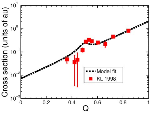
Figure 4: Differential PII cross section for an impact energy of 100 eV, as a function of the energy sharing fraction, $Q$. KL 1998 is the experimental data of Kover and Laricchia Kover and Laricchia (1998) for the triply differential cross section for an impact energy of 100 eV and ejection angle of $0^{\circ}$. The model fit has been calculated with the parameters (17) and by assuming that the triply differential cross section is the same at all ejection angles.

IV.3 Positrons in molecular Hydrogen

In the previous subsection, a model for the post-ionization energy-sharing for PII from H₂ was proposed. In this subsection, the effect of the energy sharing on transport properties is investigated for PII in rarefied H₂. The set of H₂ cross sections employed are those compiled in Bankovic et al. (2012b); Petrovic et al. (2013) and using the elastic cross section of calculated with a convergent-close-coupling formalism Zammit et al. (2013) up to $1000$ eV, extrapolating where necessary. It is clear that the ionization process, which turns on at $15.4$ eV is particularly important, and dominates at energies above $50$ eV .

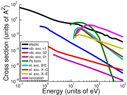
Figure 5: Cross section set for positron scattering in H₂. References are given in text.

In order to assess the importance of energy-partitioning on ionization we investigated the time-dependence of the mean energy for a source of positrons in H₂ gas at $293$ K, as they relax to thermal equilibrium in the absence of an electric field. The source distribution is chosen to be uniform in velocity space up to the $1000$ eV cutoff, which is equivalent to an initial mean energy of $600$ eV. The thermalisation profiles for the energy-partitioning model (17), and using the PII collision operator with $Q=0.5$ (equal energy-sharing), and $Q=1$ (standard excitation form) are shown in Figure 6. There are two distinct regions of rapid relaxation, one due to ionization at high energies and one due to the vibrational modes at lower energies. The first occurs on time scales of between $0.1$ and $2$ ns Amagat, while the second at about $5$ ns Amagat, which shows that the relaxation due to inelastic collisions is very rapid. While in the ionization-dominated region, the three profiles show significant differences in mean energy of up to an order of magnitude. The profile corresponding to $Q=1.0$ has the highest mean energy since the positron loses the least amount of energy during an ionization collision in that limit. It takes significantly longer to relax until the positron energies fall below the ionization region, and thus they will experience more ionization collisions. The $Q=0.5$ profile shows the lowest mean energy since the ejected electron removes large amounts of energy from the swarm, and exits the ionization region quickest. The “real” H₂ model profile sits between the even energy-sharing and standard excitation profiles as expected, since it is essentially a mixture of the two. At lower energies, once ionization collisions become insignificant, all three energy partitioning profiles coalesce, resulting in essentially the same total thermalisation times.

Although the total thermalisation time is essentially insensitive to the form of the ionization energy-partitioning, the large differences in mean energies in the ionization-dominated region can have other important effects. In a space-dependent situation, the higher mean energies can allow the positron to travel larger distances during thermalisation. This is important to PET simulations since the resolution of PET images is dependent on the distances traveled between positron emission and annihilation Czernin and Phelps (2002). Similarly, the higher the mean energy, the longer the positron swarm can significantly sample the ionization cross section, and hence the more secondary electrons that are created via PII. It is the secondary electrons created in the human body during PET scans that can cause DNA damage Sanche (2003, 2005, 2008, 2009). Furthermore, the exact energy profile of the secondary electrons will be dependent on the form of the PII energy-partitioning.

Figure 6: Mean energy temporal relaxation of a positron swarm in H₂ at 293 K. The initial source distribution is uniform in speed space up to $1000$ eV. The H₂ model ionisation parameters are given in equation (17) and are compared with constant energy sharing fractions of $Q=0.5$ and $Q=1.0$.

V Conclusion

Ionization by positron impact is a fundamentally different process than ionization by electron impact. Applications such as PET demand increasingly accurate models for positron transport, so it is important to be able to describe the ionization process in detail. To this end, a kinetic theory model with a general PII collision operator has been developed for the first time. The key feature of the ionization collision operator is the energy-partition function, which controls how the available energy is shared between the post-collision constituents.

The kinetic theory results were compared against a Monte Carlo simulation for a simple test model (11), which may serve as a new benchmark for ionization. The transport properties calculated differed between the two approaches by less than $0.6\%$ over a range of reduced electric fields and available energy fractions, which is within their respective uncertainties. The sensitivity of the transport properties to the energy-sharing fraction $Q$ for PII was shown to be significant, and much greater than that of EII. Thus large errors can result in real-world applications if PII is not treated carefully.

A simple energy-partition function was developed to capture qualitatively the underlying physics of PII. At high impact energies, the scattered positron leaves the collision with almost all of the available energy, while at near-threshold impact energies the Wannier theory Wannier (1953) suggests that the both the scattered positron and ejected electron share approximately half of the available energy. In reality, there is a slight energy-sharing asymmetry in near-threshold positron ionization Arcidiacono et al. (2005) and a more sophisticated energy-partitioning model will need to take this asymmetry into account. The model parameters were fit to the experimental results of Kover and Laricchia Kover and Laricchia (1998) for positrons in H₂ with good qualitative agreement.

Using the newly constructed H₂ energy-partitioning function, we investigated the temporal relaxation of a positron swarm from a high energy source ($600$ eV) to thermalisation at room temperature, and compared the equal-energy sharing model with the common approach of treating the PII as a standard excitation process. In the ionization-dominated region there can be more than an order of magnitude in difference in the mean energy profiles, and hence the choice of energy-partition function has a significant effect on the number of ionization collisions and the energy distribution of the secondary electrons created, which is particularly important for radiation damage modeling Sanche (2008). Our modeling also suggests that the spatial relaxation will be sensitive to the energy-partitioning, which is a topic to be further investigated.

Appendix A Derivation of positron-impact ionization operator

The case of EII has been treated by Ness Ness (1985), and we follow this work closely to derive the PII collision operator. For simplicity, we consider one ionization process with a neutral in the ground state, but the generalization is straightforward. To derive the collision operator we will consider the scattering of positrons into and out of an element of phase space, $d\mathbf{r}d\mathbf{v}$.

Let us consider a beam of positrons incident upon the background neutrals which are at rest. The flux of incident positrons, $\mathbf{I}$, in $d\mathbf{r}d\mathbf{v}$ is

$$\mathbf{I} =\mathbf{v}f\left(\mathbf{r},\mathbf{v},t\right)d\mathbf{v}.$$

If $\sigma^{\mathrm{ion}}(v)$ is the the total ionization cross section for an incoming positron of speed $v$, then the number of ionization collisions in $d\mathbf{r}d\mathbf{v}$ per unit time per neutral is,

$$I\sigma^{\mathrm{ion}}(v) =vf(\mathbf{r},\mathbf{v},t)\sigma^{\mathrm{ion}}\left(v\right)d\mathbf{v},$$

and hence, the total rate of positrons scattered out of the element $d\mathbf{r}d\mathbf{v}$ for $n_{0}$ neutral particles due to ionization is

$$J_{\mathrm{out}}^{\mathrm{ion}}(f)d\mathbf{r}d\mathbf{v} =n_{0}v\sigma^{\mathrm{ion}}(v)f(\mathbf{r},\mathbf{v},t)d\mathbf{r}d\mathbf{v}.$$ (18)

In EII, either the primary or ejected electrons (which are indistinguishable) from an ionization event somewhere else in phase space may be scattered into the element $d\mathbf{r}d\mathbf{v}.$ Since one can distinguish between electrons and positrons, the PII equivalent is simpler. Let us consider a new element of phase space with the same configuration space location but new velocity space location, i.e., $d\mathbf{r}d\mathbf{v}^{\prime}$. Similar to (18), the total number of PII in $d\mathbf{r}d\mathbf{v}^{\prime}$ per unit time is

$$n_{0}v^{\prime}\sigma^{\mathrm{ion}}(v^{\prime})f(\mathbf{r},\mathbf{v}^{\prime},t)d\mathbf{r}d\mathbf{v^{\prime}}.$$ (19)

The momentum post-ionization is shared between the scattered positron and the ejected electron. We define a quantity $B(\mathbf{v},\mathbf{v}^{\prime}),$ such that $B(\mathbf{v},\mathbf{v}^{\prime})d\mathbf{v}$ is the probability of the positron having a velocity between $\mathbf{v}$ and $\mathbf{v}+d\mathbf{v}$ after ionization, given that the incident positron has velocity $\mathbf{v}^{\prime}$. Assuming the neutral particle remains a bystander at rest during the process (to zeroth order in the mass ratio, $m/m_{0}$), then by conservation of momentum,

$$\mathbf{v}^{\prime} =\mathbf{v}+\mathbf{\bar{v}},$$

where $\mathbf{\bar{v}}$ is the velocity of the ejected electron. It follows from equation (19) and the definition of $B(\mathbf{v},\mathbf{v}^{\prime})$ that the number of positrons that enter $d\mathbf{r}d\mathbf{v}$ per unit time due to an ionization event in $d\mathbf{r}d\mathbf{v^{\prime}}$ is

$$n_{0}v^{\prime}\sigma^{\mathrm{ion}}(v^{\prime})f(\mathbf{r},\mathbf{v}^{\prime},t)B(\mathbf{v},\mathbf{v}^{\prime})d\mathbf{v}d\mathbf{r}d\mathbf{v^{\prime}}.$$

Integrating over all possible incident velocities thus yields the total rate of positrons scattered into $d\mathbf{r}d\mathbf{v}$ due to PII, i.e.,

$$J_{\mathrm{into}}^{\mathrm{ion}}(f)d\mathbf{r}d\mathbf{v} =n_{0}d\mathbf{r}d\mathbf{v}\int v^{\prime}\sigma^{\mathrm{ion}}(v^{\prime})f(\mathbf{r},\mathbf{v}^{\prime},t)B(\mathbf{v},\mathbf{v}^{\prime})d\mathbf{v^{\prime}}.$$

The total PII collision operator is then the difference in the rates of positrons scattered into and out of the element $d\mathbf{r}d\mathbf{v}$, i.e., $J^{\mathrm{ion}}=J_{\mathrm{out}}^{\mathrm{ion}}-J_{\mathrm{into}}^{\mathrm{ion}},$

$$J^{\mathrm{ion}}(f) =n_{0}v\sigma^{\mathrm{ion}}(v)f(\mathbf{r},\mathbf{v},t)-n_{0}\int v^{\prime}\sigma^{\mathrm{ion}}(v^{\prime})B(\mathbf{v},\mathbf{v}^{\prime})f(\mathbf{r},\mathbf{v}^{\prime},t)d\mathbf{v^{\prime}}.$$ (20)

If we assume central forces, then the scattering cross section and partition function are dependent only on the magnitudes of the pre- and post-collision velocities, and the angle between them, i.e., $v$, $v^{\prime}$ and $\hat{\mathbf{v}}\cdot\hat{\mathbf{v}}^{\prime}$. We may then further define a differential scattering cross section for ionization, $\sigma^{\mathrm{ion}}\left(v,v^{\prime};\hat{\mathbf{v}}\cdot\hat{\mathbf{v}}^{\prime}\right)$, such that $\sigma^{\mathrm{ion}}\left(v,v^{\prime};\hat{\mathbf{v}}\cdot\hat{\mathbf{v}}^{\prime}\right)d\mathbf{v}$ is the number of positrons scattered into the range $d\mathbf{v}$ about $\mathbf{v}$ due to incident electrons of velocity $\mathbf{v}^{\prime}$ divided by incident flux,

$$\sigma^{\mathrm{ion}}\left(v,v^{\prime};\hat{\mathbf{v}}\cdot\hat{\mathbf{v}}^{\prime}\right)d\mathbf{v} =\sigma^{\mathrm{ion}}\left(v^{\prime}\right)B\left(v,v^{\prime};\hat{\mathbf{v}}\cdot\hat{\mathbf{v}}^{\prime}\right)d\mathbf{v}.$$ (21)

The partition function satisfies a normalization condition so that

$$\sigma^{\mathrm{ion}}(v^{\prime}) =\int\sigma^{\mathrm{ion}}\left(v,v^{\prime};\hat{\mathbf{v}}\cdot\hat{\mathbf{v}}^{\prime}\right)d\mathbf{v}.$$

Substituting equation (21) into equation (20) gives the PII collision operator

$$J^{\mathrm{ion}}(f) =n_{0}v\sigma^{\mathrm{ion}}(v)f(\mathbf{v})-n_{0}\int v^{\prime}\sigma^{\mathrm{ion}}\left(v,v^{\prime};\hat{\mathbf{v}}\cdot\hat{\mathbf{v}}^{\prime}\right)f(\mathbf{v}^{\prime})d\mathbf{v^{\prime}}.$$

This operator is particle-number-conserving, i.e.

$$\int J^{\mathrm{ion}}(f)d\mathbf{v} =\int n_{0}v\sigma^{\mathrm{ion}}(v)f(\mathbf{v})d\mathbf{v}-n_{0}\iint v^{\prime}\sigma^{\mathrm{ion}}\left(v,v^{\prime};\hat{\mathbf{v}}\cdot\hat{\mathbf{v}}^{\prime}\right)f(\mathbf{v}^{\prime})d\mathbf{v^{\prime}}d\mathbf{v}$$

$$=n_{0}\int v\sigma^{\mathrm{ion}}(v)f(\mathbf{v})d\mathbf{v}-n_{0}\int v^{\prime}f(\mathbf{v}^{\prime})d\mathbf{v^{\prime}}\int\sigma^{\mathrm{ion}}\left(v,v^{\prime};\hat{\mathbf{v}}\cdot\hat{\mathbf{v}}^{\prime}\right)d\mathbf{v}$$

$$=n_{0}\int v\sigma^{\mathrm{ion}}(v)f(\mathbf{v})d\mathbf{v}-n_{0}\int v^{\prime}\sigma^{\mathrm{ion}}(v^{\prime})f(\mathbf{v}^{\prime})d\mathbf{v^{\prime}}$$

$$=0,$$

as required.

A.0.1 Legendre decomposition

For central scattering forces the partition function can be decomposed in terms of Legendre polynomials, i.e.,

$$B_{l}(v,v^{\prime}) =2\pi\int_{-1}^{1}B(\mathbf{v},\mathbf{v}^{\prime})P_{l}\left(\mu\right)d\mu,$$

where $\mu=\hat{\mathbf{v}}\cdot\hat{\mathbf{v}}^{\prime}$. For isotropic scattering, $B_{l}(v,v^{\prime})=0$ for $l\geq 1$. Multiplying equation (20) by $P_{l}\left(\cos\chi\right)$, and integrating over all angles leads to

$$J_{l}^{\mathrm{ion}}(f_{l}) =n_{0}v\sigma^{\mathrm{ion}}(v)f_{l}(v)-\begin{cases}n_{0}\int_{0}^{\infty}v^{\prime}\sigma^{\mathrm{ion}}\left(v^{\prime}\right)B_{0}(v,v^{\prime})f_{0}(v^{\prime})v^{\prime 2}dv^{\prime}&l=0,\\ 0&l\geq 1.\end{cases}$$ (22)

We now seek to represent equation (22) in terms of energy rather than speed, i.e., $U=\frac{1}{2}mv^{2}$. The probability of a positron having a speed in the range $v+dv$ after ionization, for an incident positron of speed $v^{\prime}$ is

$$v^{2}dv\int B\left(v,v^{\prime};\mathbf{\hat{v}}\cdot\mathbf{\hat{v}}^{\prime}\right)d\mbox{$\mathbf{\hat{v}}$} =B\left(v,v^{\prime}\right)v^{2}dv,$$

$$\equiv P\left(U,U^{\prime}\right)dU,$$ (23)

where $U$ and $U^{\prime}$ are the post- and pre-collision positron energies respectively, and now the right-hand-side term of equation (23) represents the probability of a positron having an energy in the range $U+dU$ after ionization for an incident positron of $U^{\prime}$. The energy partitioning function, $P(U,U^{\prime})$, has the following properties:

$$P(U,U^{\prime}) =0\ \ U^{\prime}<U+U_{I}$$

$$\int_{0}^{U^{\prime}-U_{I}}P(U,U^{\prime})dU =1\ \ U^{\prime}\geq U+U_{I}.$$

Finally, we can represent equation (22) in terms of energy and the energy-partition function, $P(U,U^{\prime})$,

$$J_{l}^{\mathrm{ion}}(f_{l}) =n_{0}\sqrt{\frac{2U}{m}}\sigma^{\mathrm{ion}}(U)f_{l}(U)-\begin{cases}\begin{array}[]{c}n_{0}\sqrt{\frac{2}{mU}}\int_{0}^{\infty}U^{\prime}\sigma^{\mathrm{ion}}\left(U^{\prime}\right)P(U,U^{\prime})f_{0}(U^{\prime})dU^{\prime}\\ 0\end{array}&\begin{array}[]{c}l=0,\\ l\geq 1,\end{array}\end{cases}$$ (24)

A.0.2 Modified Frost-Phelps operator

If the scattered positron leaves the collision with an exact fraction, $Q$, of the available energy, $U^{\prime}-U_{I}$, where $U_{I}$ is the threshold energy, then the energy-partition function has the form,

$$P(U,U^{\prime}) =\delta\left(U-Q(U^{\prime}-U_{I})\right),$$

$$=\frac{1}{Q}\delta\left(U^{\prime}-\left(\frac{U}{Q}+U_{I}\right)\right),$$

and the integral in equation (24) reduces to,

$$J_{l}^{\mathrm{ion}}(f_{l}) =\nu^{\mathrm{ion}}(U)f_{l}(U)-\begin{cases}\begin{array}[]{c}\frac{1}{Q}\frac{\left(\frac{U}{Q}+U_{I}\right){}^{\frac{1}{2}}}{U^{\frac{1}{2}}}\nu^{\mathrm{ion}}\left(\frac{U}{Q}+U_{I}\right)f_{0}\left(\frac{U}{Q}+U_{I}\right)\\ 0\end{array}&\begin{array}[]{c}l=0,\\ l\geq 1,\end{array}\end{cases}$$ (25)

where $\nu^{\mathrm{ion}}(U)=n_{0}\sqrt{\frac{2U}{m}}\sigma^{\mathrm{ion}}(U)$ is the ionization collision frequency. Equation (25) can be considered a ‘modified Frost-Phelps’ operator. A similar result for EII was given in Sigeneger and Winkler (1997). In the case where the positron gets all of the available energy, i.e., $Q=1$, equation (25) reduces to the standard Frost-Phelps operator, (6), as required. Clearly, equation (25) breaks down when $Q=0$.

Appendix B Electron impact ionization benchmarks

Transport coefficients for EII are given in Table 4, in which they are compared to the results of Ness and Robson Ness and Robson (1986). Due to the indistinguishability of post-collision particles, the results for $Q$ and $1-Q$ with respect to EII are identical, and so we consider only $Q>0.5$. The modified Frost-Phelps form of the collision operator (25) breaks down when $Q=0$, hence there is no value given in Table 4 corresponding to $Q=0$ and $Q=1$ (if one of the electrons gets the fraction $Q=1$ of the available energy, then the other receives $Q=0$ and the same problem is encountered). The EII calculations using our kinetic theory model agree closely with both our Monte Carlo simulations and the kinetic theory approach in Ness and Robson (1986). There are generally differences of less than $0.6\%$ and $0.3\%$ in the ionization rate and mean energy respectively, between the present kinetic theory results and both the Monte Carlo simulation and Ness (1985) over the whole range of reduced fields and energy sharing fractions, except for the AFE case. An error is present in the AFE calculations of Ness (1985). Values for the AFE case have been re-calculated using a similar Burnett function Kumar et al. (1980) expansion to that of Ness and Robson (which are included in Table 4 enclosed within square brackets) which agree closely with our calculations. In reference Ness (1985), the bulk drift velocities are given, which must not be confused with the flux drift velocity Sakai et al. (1977); Tagashira et al. (1977); Robson and Ness (1986). The two types of transport coefficients can be significantly different when there a non-conservative effects. Following Robson and Ness (1986) we have solved the first level of spatially-inhomogeneous equations, which come from a density gradient expansion Kumar et al. (1980), in addition to equation (4) to determine the bulk drift velocity. Both the flux and bulk drift velocities generally agree to within $0.3\%$ between the three calculation methods over the range of fields and energy-sharing fractions considered.

Table 4: Comparison of average ionization rate, $\alpha^{\mathrm{ion}}/n_{0}$, mean energies, $\epsilon$, flux drift velocities, $W_{\mathrm{flux}}$, and bulk drift velocities $W_{\mathrm{bulk}}$ for EII for model (11) for different reduced fields $E/n_{0}$ and energy sharing fractions $Q$. The first column lists the current kinetic theory calculations, the second column lists the results of our Monte Carlo simulations, and the third includes the kinetic theory calculations of Ness and Robson Ness and Robson (1986). The values enclosed in square brackets have been performed using a similar Burnett function expansion to that of Ness and Robson. $Q=\mathrm{AFE}$ corresponds to ‘all fractions equiprobably’. Note: there was an error in the AFE case in the original Ness and Robson work Ness and Robson (1986).

$E/n_{0}$		$\alpha^{\mathrm{ion}}/n_{0}$			$\epsilon$			$W_{\mathrm{flux}}$		$W_{\mathrm{bulk}}$
(Td)	$Q$	($10^{-15}$m3s-1)			(eV)			($10^{5}$ms-1)		($10^{5}$ms-1)
		Current	MC	Ness and Robson (1986)	Current	MC	Ness and Robson (1986)	Current	Ness and Robson (1986)	Current	MC	Ness and Robson (1986)
300	0		1.620	1.61		6.739	6.73		2.780		3.236	3.23
	$1/4$	1.598	1.611	1.60	6.737	6.741	6.73	2.752	2.754	3.200	3.204	3.20
	$1/3$	1.595	1.596	1.60	6.739	6.741	6.73	2.748	2.749	3.194	3.196	3.20
	$1/2$	1.591	1.589	1.59	6.742	6.744	6.74	2.744	2.745	3.189	3.192	3.19
	AFE	1.600	1.606	1.51	6.733	6.746	6.75	2.756	2.755	3.198	3.206	3.19
				[1.60]			[6.73]					[3.21]
$500$	$0$		4.643	4.68		9.009	8.99		3.920		4.752	4.74
	$1/4$	4.504	4.515	4.51	9.007	9.007	9.01	3.835	3.839	4.632	4.644	4.63
	$1/3$	4.482	4.492	4.49	9.013	9.023	9.01	3.823	3.822	4.617	4.617	4.62
	$1/2$	4.464	4.452	4.47	9.017	9.028	9.02	3.814	3.816	4.604	4.606	4.61
	AFE	4.511	4.525	4.37	9.000	9.007	9.04	3.846	3.843	4.635	4.647	4.62
				[4.52]			[9.00]					[4.64]
$800$*	$0$		9.736	9.62		13.17	13.21		5.112		6.284	6.25
	$1/4$	9.413	9.422	9.41	13.01	13.02	13.01	4.953	4.957	6.108	6.118	6.11
	$1/3$	9.357	9.372	9.37	12.99	12.99	12.99	4.933	4.936	6.090	6.092	6.09
	$1/2$	9.320	9.339	9.33	12.97	12.98	12.97	4.919	4.922	6.079	6.095	6.08
	AFE	9.461	9.445	9.20	13.03	13.02	13.09	4.968	4.976	6.137	6.137	6.12
				[9.46]			[13.02]					[6.13]