Abstract

Heavy tailed distributions present a tough setting for inference. They are also common in industrial applications, particularly with Internet transaction datasets, and machine learners often analyze such data without considering the biases and risks associated with the misuse of standard tools. This paper outlines a procedure for inference about the mean of a (possibly conditional) heavy tailed distribution that combines nonparametric analysis for the bulk of the support with Bayesian parametric modeling – motivated from extreme value theory – for the heavy tail. The procedure is fast and massively scalable. The resulting point estimators attain lowest-possible error rates and, unique among alternatives, we are able to provide accurate uncertainty quantification for these estimators. The work should find application in settings wherever correct inference is important and reward tails are heavy; we illustrate the framework in causal inference for A/B experiments involving hundreds of millions of users of eBay.com.

1 Introduction

A data generating process (DGP) is heavy tailed when the distribution on exceedances above extreme thresholds cannot be bounded by an exponential distribution. Heavy tails are common in measures of user activity on the internet (Fithian and Wager, 2015; Taddy et al., 2016). For example, Figure 2 illustrates spending, in US$ per week of bought merchandise, across 174 sets of users on eBay.com. Each sample, of 1 to 30 million users, corresponds to a treatment group in an A/B experiment. In our modal treatment group, less than 0.05% of users spend more than $2000; however, these users account for 20% of the total spending.

Figure 1: The proportion of observations (left) and of total spending (right) due to users spending greater than $2000 in each treatment group.

Figure 2: Sample distribution for user spending values below $100 in the experiments of Section 6.

Heavy tails imply that observations in high percentiles are high variance and will have a large influence on sample means. In some cases, including 2/3 of the groups we study here, the tail variance is infinite: the fitted parametric tail models imply nonexistent second moments. Even when the variance is merely near-infinite, these heavy tails have important consequences for our inference.

• The learning rate for mean inference is slower than $\sqrt{N}$, for sample size $N$, and the usual standard error estimators tend to underestimate uncertainty (e.g., Romano and Wolf, 1999).

• Gaussian error assumptions are invalid both in finite samples and asymptotically (Feller, 1971).

• Nonparametric bootstrap estimators of sampling uncertainty about the mean will fail: they are inconsistent for the true sampling distribution (Athreya, 1987).

These issues have real practical implications, and the over-sized influence of large observations on the sample mean is well recognized by practitioners who measure on-line transactions (e.g., when evaluating the treatment effect from an A/B trial). A common ad- hoc solution is to use Winsorization (Dixon, 1960) wherein values above a threshold are replaced by that threshold. However, estimation is then very sensitive to the Winsorization threshold and, due to the inconsistency of the nonparametric bootstrap, there are no tools available for its optimal selection or for uncertainty quantification. At the same time, fully parametric modeling is impractical because the transaction distributions defy summarization. Figure 2 shows that, at the low end of the spending range, the distribution is characterized by probability spikes at discrete price points (e.g., $1, $99.99) and could not be represented by any standard low-dimensional parametric family.

We resolve these issues by combining nonparametric inference for the bulk of a distribution with parametric inference for the tail above a fixed threshold. We give a theoretically motivated rule for choosing the threshold and demonstrate that inference is robust to choices around this rule. The result is a simple framework for scalable inference with heavy tailed data.

We highlight number of contributions.

Scalability:  Our algorithms provide scalable inference in a setting where this does not exist. Related Bayesian approaches have been proposed before (see below), but these do not scale to even moderately sized datasets and are completely infeasible on the Internet datasets that motivate our work. In contrast, we require no more computation on the bulk of the data than estimation of sample means and variance, and our tail inference is available via either analytical or efficient computational approximation.

Inference:  Our posterior mean estimators achieve the lowest error rates available. Moreover, our posterior standard deviations on distribution means are an accurate measure of the frequentist standard error. Indeed, they outperform any other available standard error estimators. There exist other good and scalable point estimators for the means of heavy tailed distributions, but none come with reliable uncertainty quantification (which is essential in the motivating A/B trial applications).

Consistency:  It is well known (Athreya, 1987) that the usual nonparametric bootstrap is inconsistent as an estimator for the sampling distribution of the mean of a heavy tailed distribution. We introduce a novel semiparametric bootstrap and show that it is consistent for a tail threshold that grows with the sample size. Our Bayesian inference algorithm is closely related to this semiparametric bootstrap.

Bootstrap-based posterior sampling:  For inference about the tail parameters, we present a novel independence Metropolis Hastings (iMH) algorithm that samples from the posterior through adjustment of the results from a parametric bootstrap. The algorithm is trivial to code, fast and parallelizable, and its acceptance rate is a measure of the distance between Bayesian and frequentist inference.

Extreme value analysis:  We contribute two general points on Bayesian analysis of heavy tails. First, our consistency analysis provides a rule for choosing the tail threshold and in both theory and practice we find that results are robust around this rule. The threshold can thus be conditioned upon in the posterior, leading to much simpler inference than is possible if it is treated as a random variable. Second, we find significant gains from use of informative priors on the tail index and propose a scheme for specification based upon a larger background dataset. Informative priors on the tail scale make little difference in comparison.

Section 2 defines our general framework, Section 3 details the parametric tail analysis, and Section 4 studies consistency. We illustrate our methods in analysis of A/B experiments involving more than 100 million users of eBay.com: Section 6 validates performance through subsampling of treatment groups, and Section 7 studies inference on treatment effects in A/B trials.

1.1 Related Literature

A related Bayesian approach is proposed in Nascimento et al. (2012): they combine a Dirichlet process mixture below a threshold with a generalized Pareto above. All parameters, including the value of the threshold itself, are sampled from their joint posterior in an MCMC algorithm. Unfortunately, this procedure is completely non-scalable; it takes around 1 second per posterior draw when analyzing one of the small subsamples from Section 6. The continuous mixture model is also a poor fit for Internet transaction datasets, which include density spikes at discrete values (e.g., $0.99, $99). In any case, the MCMC failed to converge without tight priors on the tail threshold or scale, and yields poorly performing estimators with errors larger than those from the naive sample mean.

Johansson (2003) describes estimation for the mean of a heavy tailed distribution that combines the sample mean below a threshold with the mean of a maximum likelihood generalized Pareto above that threshold. The point estimates from this approach are equivalent to those from our procedure under the non-informative prior with Laplace posterior approximation. Johansson’s asymptotic variance formulas depend upon unknown model parameters and thus cannot be applied in practical inference.

Romano and Wolf (1999) use without-replacement sub-sampling to estimate the sampling distribution for the mean of a heavy tailed sample. We discuss and compare to their estimators in our applications.

Finally, Fithian and Wager (2015) estimate tail distributions through exponential tilting of models fit on larger samples. This shares with our informative-prior models a strategy of using background datasets to inform individual tails. Their tilting estimator works nicely: it provides point estimation that is as good as our best methods. However, there is no uncertainty quantification available in Fithian and Wager (2015).

2 A Semiparametric model for heavy tailed data generating processes

Our inference strategy is built around the use of Dirichlet-multinomial sampling as a flexible representation for an arbitrary data generating process (DGP). In its standard application, this model treats the observed sample as a draw from a multinomial distribution over a large but finite set of support points. A Dirichlet prior is placed on the probabilities in this multinomial, and the posterior distribution over possible DGPs is induced by the posterior on these probabilities. The approach has a long history. It was introduced by Ferguson (Ferguson, 1973), it serves as the foundation for the Bayesian bootstrap (Rubin, 1981), and it has been studied by numerous authors (Chamberlain and Imbens, 2003; Lancaster, 2003; Poirier, 2011; Taddy et al., 2015, 2016).

Our work presents an extension of the standard Dirichlet-multinomial scheme. Consider a univariate random variable, say $z$. We assume the usual fully-nonparametric model below a certain fixed threshold, say $u$. That is, the prior DGP for $z<u$ is a Multinomial draw, with Dirichlet distributed probability, from a large-but-finite number of support points. At the same time, with some probability our realized $z$ is instead drawn as $u+v$ where $v>0$ is a random exceedance from some distribution.

We model our tail exceedances as realizations from a generalized Pareto distribution (GPD), with $\mathrm{p}(V<v)=1-(1+\xi v/\sigma)^{-1/\xi}$ and density function on $v>0$

$$\mathrm{GPD}(e;~{}\xi,~{}\sigma)=\frac{1}{\sigma}\left(1+\xi\frac{v}{\sigma}\right)^{-(\frac{1}{\xi}+1)}$$ (1)

for tail index $\xi>0$ and scale $\sigma>0$. The generalized Pareto is a commonly applied tail model (Smith, 1989; Davison and Smith, 1990; Pickands, 1994; Johansson, 2003; Fithian and Wager, 2015) with justification as the limiting distribution for exceedance beyond large $u$ for a wide family of processes (Pickands, 1975; Smith, 1987; Coles and Tawn, 1996). As $\xi\rightarrow 0$ the GPD converges to an exponential distribution, and for $\xi>0$ the tails are heavier-than-exponential. For $\xi\geq 1/2$ the variance of $v$ is infinite, and for $\xi\geq 1$ the mean is infinite. Our analysis focuses on $\xi\in(0,1)$, so that the tail is heavy enough to cause problems but not so heavy that the mean does not exist.

Combining the GPD and Dirichlet-multinomial sampling yields our semi-parametric model,

$$g(z)=\frac{1}{|\boldsymbol{\theta}|}\sum_{l=1}^{L}\theta_{l}\mathds{1}_{[z=\zeta_{l}]}+\frac{\theta_{L+1}}{|\boldsymbol{\theta}|}\mathrm{GPD}(z-u;~{}\xi,~{}\sigma)\mathds{1}_{[z\geq u]}$$ (2)

where $\boldsymbol{\mathcal{Z}}=\{\zeta_{1}\dots\zeta_{L}\}$, all elements less than $u$, is the support for the bulk of the DGP $g(z)$, $\boldsymbol{\theta}=[\theta_{1}\cdots\theta_{L+1}]^{\prime}$ is a vector of random weights with $\theta_{l}\geq 0\;\forall\;l$, and $|\boldsymbol{\theta}|=\sum_{i}|\theta_{i}|$.

Observations are assumed drawn independently from (2) by first sampling $l_{i}$ with probability $\theta_{l_{i}}$ and then assigning $z_{i}=\zeta_{l_{i}}$ for $l_{i}\leq L$ and otherwise drawing $z_{i}-u\sim\mathrm{GPD}$. A posterior over $g$ is induced by the posterior over the model parameters: $\boldsymbol{\theta}$, $\xi$, and $\sigma$. Functionals of $g$, such as $\mathds{E}_{g}f(z)$ for arbitrary function $f$ and where $\mathds{E}_{g}$ implies expectation over $z\sim g$, are thus random variables.

2.1 Inference on the sampling weights

A conjugate prior places independent exponential distributions on each weight: $\theta_{l}\sim\mathrm{Exp}(a)$ for $l=1\dots L+1$, where $\mathds{E}[\theta_{l}]=a$ and $a>0$ is the prior ‘rate’. After observing a sample $\mathbf{Z}=[z_{1}\cdots z_{N}]^{\prime}$, each weight remains independent in the posterior with distribution $\theta_{l}|\mathbf{Z}\sim\mathrm{Exp}(a+\sum_{i=1}^{N}\mathds{1}_{[l_{i}=l]})$. We focus on the limiting prior that arises as $a\rightarrow 0$ (Rubin, 1981; Chamberlain and Imbens, 2003; Taddy et al., 2015, 2016). This ‘non-informative’ limit yields a massive computational convenience: as $a\rightarrow 0$ the weights for unobserved support points converge to a point mass at zero: $p(\theta_{l}=0|\mathbf{Z})=1$ if $l\neq l_{i}$ $\forall i$. Our posterior is then a multinomial sampling model with random positive weights on only the observed data points and on the tail ($l_{i}=L+1$).

To simplify notation, say $z_{i}<u$ for $i\leq m$ and $z_{i}\geq u$ for $i=m+1,\dots,m+n$ with $N=m+n$. We then overload and re-write $\boldsymbol{\theta}=[\theta_{1},\dots,\theta_{m},\theta_{m+1}]^{\prime}$ as the posterior vector of weights on observations $z_{1},\dots,z_{m}$ (all less than $u$; repeated values are fine) and on the tail. A posterior DGP realization is

$$g(z)\mid\mathbf{z},\xi,\sigma= \frac{1}{|\boldsymbol{\theta}|}\sum_{i=1}^{m}\theta_{i}\mathds{1}_{[z=z_{i}]}+$$

$$+\frac{\theta_{m+1}}{|\boldsymbol{\theta}|}\mathrm{GPD}(z-u;~{}\xi,~{}\sigma)\mathds{1}_{[z\geq u]},$$ (3)

with $\theta_{i}\stackrel{{\scriptstyle iid}}{{\sim}}\mathrm{Exp}(1)~{}\forall i\leq m~{}~{}\text{and}~{}~{}\theta_{m+1}\sim\mathrm{Exp}(n)$. Details on the GPD tail posterior are in Section 3.

2.2 Inference on the DGP Mean

The mean of $g(z)$ is the random variable $\mu=\mathds{E}z=\left(\sum_{i=1}^{m}\theta_{i}z_{i}+\theta_{m+1}(u+\sigma(1-\xi)^{-1}\right)/{|\boldsymbol{\theta}|}.$ Uncertainty about $\mathds{E}z$ is induced by the posterior on $\boldsymbol{\theta}$ and on the mean exceedance $\lambda=\sigma/(1-\xi)$. Because $u$ is fixed, we have $\boldsymbol{\theta}\perp\!\!\!\perp\lambda$. It is easy to see that $\mathds{E}\mu=\tfrac{1}{m+n}\sum_{i=1}^{m}z_{i}+\frac{n}{m+n}(u+\mathds{E}\lambda)$.

The law of total variation yields posterior variance $\mathrm{var}\mu=\mathds{E}[\mathrm{var}(\mu|\lambda)]+\mathrm{var}(\mathds{E}[\mu|\lambda]).$ Given properties of the Dirichlet posterior on $\boldsymbol{\theta}/|\boldsymbol{\theta}|$, the first term is

$$\mathds{E}[\mathrm{var}(\mu|\lambda)]= \frac{\sum_{i=1}^{m}(z_{i}-\mathds{E}\mu)^{2}+n(u+\mathds{E}\lambda-\mathds{E}\mu)^{2}}{(m+n)(m+n+1)}$$

$$+\frac{n^{2}(m+n-2)\mathrm{var}(\lambda)}{(m+n)^{2}(m+n+1)}$$ (4)

where $\mu_{\lambda}=\left[\sum_{i=1}^{m}z_{i}+n(u+\lambda)\right]/(m+n)$ and $\mathds{E}\mu$ is the posterior expectation from above. The second term is $\mathrm{var}(\mathds{E}[\mu|\lambda])=\frac{n^{2}}{(m+n)^{2}}\mathrm{var}(\lambda)$and the full expression

$$\mathrm{var}\mu= \frac{\sum_{i=1}^{m}(z_{i}-\mathds{E}\mu)^{2}+n(u+\mathds{E}\lambda-\mathds{E}\mu)^{2}}{(m+n)(m+n+1)}$$

$$+\frac{2n^{2}(m+n-0.5)}{(m+n)^{2}(m+n+1)}\mathrm{var}(\lambda).$$ (5)

Noting that $\lambda=\sigma/(1-\xi)$, the necessary tail moments $\mathds{E}\lambda$ and $\mathrm{var}(\lambda)$ are available through either Laplace approximation or MCMC as described below.

3 Inference for tail parameters

In this section we describe Bayesian modeling and inference for the GPD parameters, $\xi$ and $\sigma$, conditional upon the sample of exceedances $\{v_{i}=z_{m+i}-u\}_{1}^{n}$. We are focusing on heavy tails with finite mean exceedances that correspond to $\xi\in(0,1)$. On this range, $\sigma$ can take any positive value. A simple independent prior setup is then $\pi(\sigma,\xi)=\mathrm{Beta}(\xi;a,b)\mathrm{Ga}(\sigma;c,d)\propto\xi^{a-1}(1-\xi)^{b-1}\sigma^{c-1}e^{-d\sigma}$, where $\mathrm{Beta}(\cdot~{};~{}a,b)$ denotes a beta density with mean $a/(a+b)$ and $\mathrm{Ga}(\cdot~{};~{}c,d)$ a gamma density with mean $c/d$, with $a,b,c,d>0$. We work primarily with a version of this prior takes the limit $c,d\rightarrow 0$ to obtain

$$\pi(\sigma,\xi)=\frac{1}{\sigma}\xi^{a-1}(1-\xi)^{b-1}\mathds{1}_{\xi\in(0,1)},$$ (6)

the combination of a beta on $\xi$ and an improper uniform prior on $\log\sigma$. Following results in Northrop and Attalides (2015) and Castellanos and Cabras (2007), the posterior for $[\sigma,\xi]$ will be proper under this prior given a minimum of three observations.

Our beta-gamma prior combines with the GPD likelihood to yield a log posterior proportional to $l(\sigma,\xi)=-\frac{1+\xi}{\xi}\sum_{i}\log\left(1+\xi\frac{v_{i}}{\sigma}\right)+(a\!-\!1)\log\xi+(b\!-\!1)\log(1\!-\!\xi)+(c\!-\!n\!-\!1)\log\sigma-d\sigma.$ Maximization of this objective leads to MAP estimates of the parameters, say $[\hat{\xi},\hat{\sigma}]$. The related problem of MLE estimation for GPDs is well studied by Grimshaw (1993) and his algorithm is easily adapted for fast MAP estimation within our domain $[\xi,\sigma]\in(0,1)\times\mathds{R}^{+}$.

3.1 Laplace posterior approximation

For fast approximate inference, this section proposes analytic posterior approximation via Laplace’s method centered on the posterior mode. The main object of interest is the posterior for the GPD mean, $\sigma/(1-\xi)$. We make the transformation

$$\lambda=\frac{\sigma}{1-\xi}\Leftrightarrow\sigma=\lambda(1-\xi),$$ (7)

with inverse Jacobian $|J|=1-\xi$, to obtain the posterior

$$\mathrm{p}( \lambda,\xi\mid\mathbf{v})\propto$$ (8)

$$\frac{\xi^{a-1}e^{-d\lambda(1-\xi)}}{\lambda^{n-c+1}(1-\xi)^{n-b-c+1}}\prod_{i}\left(1+\frac{\xi}{1-\xi}\frac{v_{i}}{\lambda}\right)^{-\left(\frac{1}{\xi}+1\right)}.$$

Note that the MAP estimate for $\lambda$ is just $\hat{\lambda}=\hat{\sigma}/(1-\hat{\xi})$. The Laplace approximation (Tierney and Kadane, 1986) to the marginal posterior distribution on $\lambda$ is available as $\mathrm{\hat{p}}\left(\lambda\mid\mathbf{x}\right)=\mathrm{N}\left(\hat{\lambda},-\left.\nabla_{\lambda\lambda}^{-1}\right|_{\left[\hat{\lambda},\hat{\xi}\right]}\right),$where $\nabla_{\lambda\lambda}$ is the curvature of the log posterior with respect to $\lambda$ via $\displaystyle\frac{\partial\log\mathrm{p}(\lambda,\xi|\mathbf{v})}{\partial\lambda}=$

$$\nabla_{\lambda}=\frac{1}{\lambda}\left[(1/\xi+1)\sum_{i}q_{i}-n+c-1\right]-d(1-\xi)$$

where $q_{i}=\xi v_{i}/\left[(1-\xi)\lambda+\xi v_{i}\right]$). The approximate variance for $\lambda$ is, with $\hat{q}_{i}=\hat{\xi}v_{i}/\left[(1-\hat{\xi})\hat{\lambda}+\hat{\xi}v_{i}\right]$,

$$\widehat{\mathrm{var}}(\lambda\mid\mathbf{x})=-\!\hat{\lambda}^{2}\!\left[n-\!c+\!1\!+\!\left(\frac{1}{\hat{\xi}}\!+\!1\right)\sum_{i}\left(\hat{q}_{i}^{2}\!-\!2\hat{q}_{i}\right)\right]^{\!-1}\!\!\!.$$

3.2 Posterior sampling and approximation

For full posterior inference, we propose a novel independence Metropolis Hastings (iMH) algorithm (e.g., Gamerman and Lopes, 2006) that uses a parametric bootstrap of the MAP estimates as an MCMC proposal distribution. This approach is similar to the bootstrap reweighting of Efron (2012), but unlike that work it does not require an analytic expression for the sampling distribution of the statistics of interest.

Bootstrap iMH posterior sampler

• Fit the MAP parameter estimates $[\hat{\xi},\hat{\sigma}]$ to maximize the log posterior objective $l(\xi,\sigma)$.

• Draw $\{\hat{\xi}^{b},\hat{\sigma}^{b}\}_{b=1}^{B}$ from the parametric bootstrap:

  • Generate a sample $\{z_{i}^{b}\}_{i=1}^{n}$ by simulating from the MAP estimated model $\mathrm{GPD}(\hat{\xi},\hat{\sigma})$.

  • Obtain new MAP estimates $[\hat{\xi}^{b},\hat{\sigma}^{b}]$ conditional upon $\{z_{i}^{b}\}_{i=1}^{n}$.

• Estimate the bootstrap distribution, say $r(\xi,\sigma)$, via kernel smoothing on $\{\hat{\xi}^{b},\hat{\sigma}^{b}\}_{b=1}^{B}$.

• For $b=2\dots B$, replace $[\hat{\xi}^{b},\hat{\sigma}^{b}]$ with $[\hat{\xi}^{b-1},\hat{\sigma}^{b-1}]$ with probability

  $$1-\mathrm{min}\left\{\frac{r(\hat{\xi}^{b-1},\hat{\sigma}^{b-1})\exp[l(\hat{\xi}^{b},\hat{\sigma}^{b})]}{r(\hat{\xi}_{b},\hat{\sigma}_{b})\exp[l(\hat{\xi}^{b-1},\hat{\sigma}^{b-1})]},~{}1\right\}.$$

This is simple and fast. It also connects Bayesian and frequentist inference: high acceptance rates imply a posterior close to the sampling distribution. We emphasize that this is a novel recipe for generating MCMC algorithms from bootstrap samples, and due to the often close relationship between sampling distributions and posteriors we expect that this recipe will be useful in a wide variety of additional settings.

3.3 Background tails and informative priors

It is common to expect similar tail properties across multiple distributions. For example, we believe that small changes to the eBay website have negligible effect on whether a user makes a big purchase. This information can be used in a prior that shrinks each tail towards a larger background dataset.

We focus on adding information on the tail index, $\xi$, under the prior in (6). The tails of related distributions tend to converge to a GPD with the same index (Pickands, 1975) and there is abundant precedence for analysis of multiple distributions using a shared tail index (Davison and Smith, 1990; Fithian and Wager, 2015). If you believe that every group has the same tail index, use as your prior for $\xi$ the posterior from analysis of a larger dataset. Applying the methods of Section 3 to 100,000 users with spending over $2000, we obtain a posterior, and hence prior, on $\xi$ that is well approximated by a $\mathrm{Beta}(80,80)$ distribution. Alternatively, if you believe that each treatment group has a different-but-similar tail index, specify the $\mathrm{Beta}(a,b)$ distribution that best fits a sample of estimated tail indexes from prior analyses. In our eBay example, considering a set of 149 $\hat{\xi}$ from samples not analyzed in Sections 6 –7, this yields a $\mathrm{Beta}(9,9)$ prior.

In Section 6 we find that both priors – the hierarchical-model $\mathrm{Beta}(9,9)$ and the single-background-tail $\mathrm{Beta}(80,80)$ – lead to significant improvements in estimation. In contrast, we generally do not recommend using an informative prior on $\sigma$. The theory of Section 4 implies that this scale parameter is sensitive to $u$, so that information at one threshold does not inform estimation at another. Experimentation under the setup of Section 6 for priors on $\sigma$ (not shown) generally led to higher errors and lower ratios of the posterior standard deviation relative to the true error rate.

4 Consistency of the semiparametric heavy tailed bootstrap

Consider inference about $Q_{N}=\sqrt{N}(\hat{\mu}_{N}-\mu)$ for a sample of $N$ observations drawn from true distribution function $F(z)$, with $\int_{0}^{\infty}zdF(z)=\mu<\infty$ and where $\hat{\mu}_{N}$ denotes the MLE of $\mu$ for a size-$N$ sample from $F$. A bootstrap replaces $F\approx\widehat{F}_{N}$ and uses this to obtain $b=1,\ldots,B$ draws of $Q_{N}^{b}=\sqrt{N}(\hat{\mu}_{N}^{b}-\hat{\mu}_{N})$ where $\hat{\mu}_{N}^{b}$ is the MLE for a size-$N$ sample from $\widehat{F}_{N}$. The targeted sampling distribution, $G_{N}(q)=\mathrm{p}(Q_{N}<q)$, is estimated as $\widehat{G}_{N}(q)=B^{-1}\sum_{b=1}^{B}\mathds{1}_{[Q^{b}_{N}<q]}$.

Standard results (Bickel and Freedman, 1981; Beran, 2003) require that $\widehat{G}_{N}$ converges in distribution to $G_{\infty}$ uniformly across all $\widehat{F}_{N}$ in a neighborhood, say $\mathcal{F}$, containing $F$ and also $\widehat{F}_{N}$ for $N$ big enough (in addition, the mapping $F\mapsto G_{\infty}$ must be continuous). Convergence in probability for $\widehat{F}_{N}(z)$ to $F(z)$ $\forall z$ then implies consistency of $\widehat{G}_{N}$ in that, as $N\to\infty$, $\mathrm{p}(|\widehat{G}_{N}(q)-G_{N}(q)|<\epsilon)\to 0$ for all $q$ and $\epsilon>0$.

Athreya (1987) shows that the nonparametric bootstrap – using the empirical distribution function (EDF) as $\hat{F}_{N}$ – is inconsistent for the distribution of the sample mean for data that has infinite variance. As explained by Hall (1990), in this setting $\widehat{G}_{N}$ based upon samples from $\hat{F}_{N}$ does not converge uniformly to $G_{\infty}$ because sums of the largest re-sampled observations, $\sum_{i=N-r}^{N}z^{b}_{(i)}$ for $r\geq 1$, can be dominated by repeats of the largest sample observation, $z_{(N)}$.

Instead, define a semiparametric bootstrap that is the frequentist analogue of our Bayesian procedure.

Semiparametric Frequentist Bootstrap

Given MLE parameters, $[\hat{\xi}_{n},\hat{\sigma}_{n}]$, for $b=1,\ldots,B$:

• draw $m_{b}\sim\mathrm{Bin}(m/N,N)$ and set $n_{b}=N-m_{b}$;

• sample with replacement $m_{b}$ observations from $\{z_{i}:z_{i}<u\}$, say $\{z^{b}_{1},\ldots,z^{b}_{m_{b}}\}$;

• draw $v^{b}_{1}\ldots v^{b}_{n_{b}}$ from $\mathrm{GPD}(\hat{\xi}_{n},\hat{\sigma}_{n})$ and fit the corresponding MLE, $\hat{\lambda}^{b}_{n_{b}}=\hat{\sigma}^{b}_{n_{b}}/(1-\hat{\xi}^{b}_{n_{b}})$;

• set $\hat{\mu}^{b}_{N}=\left(\sum_{i=1}^{m_{b}}z_{i_{b}}+n_{b}(u+\hat{\lambda}^{b}_{n_{b}})\right)/N$.

The sampling distribution, e.g., for $\sqrt{N}(\hat{\mu}_{N}-\mu)$ is then approximated by $\left\{\sqrt{N}(\hat{\mu}_{N}^{b}-\hat{\mu}_{N})\right\}_{b=1}^{B}$.

This semiparametric bootstrap is the combination of three bootstrap estimators, for distributions on $\frac{1}{m}\sum_{i=1}^{N}z_{i}\mathds{1}_{[z_{i}<u]}$, on $m/N$, and on $\hat{\lambda}_{n}$. Consistency of the nonparametric bootstrap for the first two statistics is established through standard arguments (Mammen, 1992). Therefore, to show consistency for the semiparametric bootstrap we need only to confirm that the bootstrap using $\widehat{F}_{N}(z-u|z\geq u)=\mathrm{GPD}(\hat{\xi}_{n},\hat{\sigma}_{n})$ converges to the correct distribution for $\hat{\lambda}_{n}$.

Johansson (2003) considers DGPs with distribution functions $F(z)=1-cz^{-1/\zeta}(1+z^{-\delta}L(z))$, where $c,\delta>0$ and $L(tz)/L(z)\to 1$ with $z\to\infty$ for $t>0$. This defines a wide class of heavy tailed distributions, and for $u_{N}$ large enough the distribution $F(z-u_{N}|z\geq u_{N})$ approaches a $\mathrm{GPD}(\xi,\sigma_{N})$ where $\sigma_{N}=u_{N}\xi$. Following the same steps as Johansson, which apply results from Smith (1987) on the asymptotic distribution for MLEs $[\hat{\xi}_{n},\hat{\sigma}_{n}]$, you can show that for $F(z)$ with $\xi\in(0,1)$ and $z^{-\delta}L(z)$ non-increasing, if $u_{N}=O(N^{\xi/(1+2\delta\xi)})$ then

$$\sqrt{n}\left(\hat{\lambda}_{n}-\mathds{E}_{F}[z-u_{N}|z\geq u_{N}]\right)\rightarrow_{d}\mathrm{N}(0,q_{n})$$ (9)

where $q_{n}=\hat{\sigma}_{N}(1+\xi)(1-\xi+2\xi^{2})/(1-\xi)^{4}$. Thus our bootstrap sample generator, $\mathrm{GPD}(\hat{\xi}_{n},\hat{\sigma}_{n})$, converges to $F(z-u_{N}|z\geq u_{N})$ along a sequence of distributions with means $\hat{\lambda}_{n}$ that are asymptotically normal around the target, $\mathds{E}_{F}[z-u_{N}|z\geq u_{N}]$. From Beran (1997), this establishes consistency of the tail bootstrap, and hence of our full semiparametric bootstrap.

The bootstrap succeeds here because MLEs converge quickly to the ‘true’ GPD model; inference is then based upon new samples from this distribution and, unlike resamples from the EDF, these are not overly influenced by high order statistics in the original sample. From (9), so long as $u_{N}$ is growing at the right rate our true tail is converging to a GPD with $\sigma_{N}=\xi u_{N}$. We can use this fact and the estimated ratio $\hat{\sigma}/(\hat{\xi}u)$, over a set of candidate $u$, to guide threshold selection.

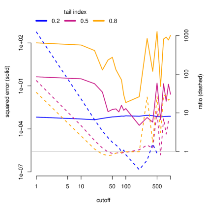
Figure 3: Mean estimation error (solid) and estimated ratio $\hat{\sigma}/(\hat{\xi}u)$ for tail thresholds $u$ and indices $\xi$.

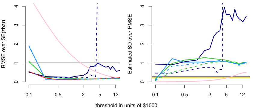
– Bayes a,b=1 – Bayes a,b=9 – Bayes a,b=80 – Winsorization – tilting – sample mean – N/2 subsampling

Figure 4: Average performance, over 100 samples of N=50,000 from each of two eBay treatment groups, as function of threshold $u$. Our semiparametric Bayesian procedure is shown for different $\mathrm{Beta}(a,b)$ priors on $\xi$, with iMH solid and Laplace dashed, against results for naive sample means, Winsorized means, the tilting of Fithian and Wager (2015), and $N/2$ subsampling standard error estimation. The left panel shows RMSE on the full sample mean relative to performance of the naive sample mean; the right panel shows estimated standard deviations relative to the corresponding ‘true’ RMSE from the left.

5 Simulations

To illustrate our techniques and the guidance for choosing $u$, we study simulated data from a combination of exponential and GPD distributions. In each simulation, we draw $10^{5}$ from an $\mathrm{Exp}(10)$ distribution and to half of these we add a draw from a $\mathrm{GPD}(\xi,10)$.

We consider three tail indices, $\xi\in\{0.2,0.5,0.8\}$, that span from a near-exponential tail – where the naive sample mean is a fine estimator – to a heavy tail with infinite variance. We apply our iMH semiparametric analysis under a range of threshold values. Results are shown in Figure 3. In each case, the estimated ratio $\hat{\sigma}/(\hat{\xi}u)$ drops below one – the value which our theory in Section 4 indicates we should target – before rising above one and becoming unstable. In the light tailed case, the error is mostly unaffected by $u$. For the two heavy tails – $\xi\geq 0.5$ – the error is lowest around the point when $\hat{\sigma}/(\hat{\xi}u)$ is equal to one and increasing in $u$. Thus, our rule for choosing $u$ is to find the value where this ratio is near one and increasing.

6 Performance study

Even in the presence of infinite variance and other difficulties, one can reliably measure relative performance by comparing estimators trained on small subsamples to the corresponding full sample statistic (Politis and Romano, 1994; Bickel et al., 1997). We apply this approach on two independent eBay treatment groups, each containing more than $10^{7}$ observations above $0. For 100 repetitions on each group, we draw a subsample of $N=$50,000 and obtain, for each algorithm under study, a mean estimate based upon this subsample. This estimate is compared to the full-sample average, $\bar{z}$, and we report the discrepancy.

Figure 5: Treatment effect estimates in four A/B trials from eBay. The Bayesian posterior is the region in blue, Winsorized estimation is in black, and the naive sample estimator is in red. Points and lines are point estimates and intervals are $\pm 1\mathrm{sd}$ or $\pm 1\mathrm{se}$, as appropriate.

Resulting averages are shown in Figure 4 across a range of thresholds and we make several remarks.

$\bullet$ The two semiparametric Bayesian analyses with informative priors on the tail index – $\xi\sim\mathrm{Beta}(9,9)$ and $\mathrm{Beta}(80,80)$ – provide superior estimation over a wide range of thresholds $u$. Their posterior means (from either Laplace or iMH) have the lowest or near-lowest RMSE – around 20-40% of the sample mean RMSE – in both datasets for $u$ above $500.

$\bullet$ The non-informative prior – $\xi\sim\mathrm{Beta}(1,1)$ – also leads to much lower RMSE than the sample mean for thresholds below $4000. However, at higher thresholds it gives larger errors than the informative prior schemes. The iMH RMSE is still an improvement on the sample mean, but the Laplace approximation under this non-informative prior fails dramatically: RMSE explodes by an order of magnitude at high thresholds. Since Laplace approximation under the non-informative prior is practically equivalent to the MLE estimator of Johansson (2003), we see that such techniques give terrible results for poorly chosen $u$.

$\bullet$ The semiparametric Bayesian analyses are the only procedures that give accurate quantification of frequentist sampling variability. For $u>$ $500, the two informative priors lead to posterior standard deviations that are near the observed RMSE over our 200 subsamples. For the $\mathrm{Beta}(80,80)$ prior, both Laplace and iMH standard deviations are within 10% of the true RMSE. The $\mathrm{Beta}(9,9)$ prior does worse but is still better than any alternative. The $\mathrm{Beta}(1,1)$ prior with iMH sampling also provides accurate uncertainty quantification, but over the more narrow range of $u\in(\$100,\$1000)$. In each case, our rule-of-thumb ratio $\hat{\sigma}/(\hat{\xi}u)$ is around one in these regions.

$\bullet$ For the informative priors, Laplace and iMH procedures give nearly identical RMSE for their mean estimates (the dashed and solid lines are on top of each other) but iMH standard deviations do a slightly better job replicating the observed RMSE. As may be expected, the discrepancy between Laplace and iMH results decreases with prior information. Also, acceptance rates on the iMH sampler were above 90% except at extreme thresholds, indicating that our Bayesian procedure is converging towards inference from a semiparametric frequentist bootstrap.

$\bullet$ The tilting procedure of Fithian and Wager (2015), using the same background sample behind our $\mathrm{Beta}(80,80)$ prior, yields low RMSEs at a wide range of $u$. This takes longer to run than 1000 iMH draws, but still finishes in seconds. Unfortunately, there is no uncertainty quantification available.

$\bullet$ Winsorization does poorly. Its RMSE is larger than that of the sample mean until $u>\$2000$. The associated standard errors – Winsorized standard deviation over $\sqrt{N}$ – are always too small.

$\bullet$ Unplotted, we find that use of only the GPD model (i.e., setting $u=0.01$) leads to RMSEs 5-20 times larger than that of the sample mean. This could be predicted from the histogram in Figure 2, which shows the sample of spend values below $100 looking nothing like a sample from a GPD (or any continuous density).

$\bullet$ Naive standard errors for the sample mean – $\mathrm{sd}(z)/\sqrt{N}$ – are around 1/3 the observed RMSE. The subsampling standard-error estimators from Romano and Wolf (1999), using subsamples of size $N/2$ and estimated learning rate $N^{\min(0.5,1-\hat{\xi})}$ for MLE $\hat{\xi}$, lead to standard errors that are still around 70% too small.

Our Bayesian semiparametric procedure, especially with some prior information for the tail index, provides lowest-possible RMSE and accurate uncertainty quantification. Both iMH and Laplace schemes are fully scalable, but Laplace is essentially free and under the informative prior it is practically indistinguishable from the slightly more expensive iMH.

7 A/B experiments

Finally, we turn to the motivating application for these ideas. In A/B experiments at eBay, two independent heavy tailed samples are obtained: one from a group receiving a treatment and another from a control group. The object of interest is $\gamma=\mu_{1}-\mu_{0}$ where $\mu_{1}$ is the mean of the treatment group and $\mu_{0}$ the mean of the control group. The samples are independent, so that variance on $\gamma$ is the sum of group mean variances.

Results are shown in Figure 5 for four example experiments. The Bayesian estimation here uses our informative $\mathrm{Beta}(80,80)$ prior and the uncertainty bounds are based upon the Laplace approximation. In each case, point and uncertainty estimates for the average treatment effects are remarkably stable across thresholds. In contrast, Winsorized estimators can change rapidly with $u$ and their standard errors are always low relative to the Bayesian standard deviations. We also show the naive mean and standard error estimates. In all but one case, this yields an uncertainty interval that is qualitatively different from the Bayesian posterior; in two cases, our semiparametric procedure moves the treatment effect from looking possibly significant to insignificant, and visa versa.

8 Conclusion

Big Data is exciting because it allows us to estimate tiny and complicated signals. However, even with massive amounts of data you need to be careful about inference in the presence of heavy tails. Instead of turning to a full modeling framework, which would be impractical on datasets of this size and complexity, we use simple nonparametrics for the easy bit (the middle of the distribution) while applying careful parametric modeling on the hard bits (the tail). Although the novel iMH sampler is fast and simple (and provides a nice connection to frequentist inference), with prior information about the tail index you can avoid sampling altogether. The procedure is massively scalable.

We have focused on single distributions (and comparisons between pairs), but the work here is applicable in many more complex modeling scenarios. For example, any bandit learning scheme (e.g., Scott, 2010) requires accurate uncertainty quantification for the posterior distribution of rewards; when these rewards come with a heavy tail, our approach should be used. As another example, bagging procedures such as random forests will tend to over-fit in the presence of extreme values (Wyner et al., 2015). Our methods can be used to define a semiparametric loss function at leaf nodes.

References

- Athreya [1987] KB Athreya. Bootstrap of the mean in the infinite variance case. The Ann. of Stat., 15:724–731, 1987.
- Beran [1997] R Beran. Diagnosing bootstrap success. Ann. of the Institute of Stat. Math., 49:1–24, 1997.
- Beran [2003] R Beran. The impact of the bootstrap on statistical algorithms and theory. Stat. Science, 18:175–184, 2003.
- Bickel and Freedman [1981] P Bickel and D Freedman. Some asymptotic theory for the bootstrap. Ann. of Stat., 9:1196–1217, 1981.
- Bickel et al. [1997] PJ Bickel, F Götze, and WR van Zwet. Resampling fewer than n observations: gains, losses, and remedies for losses. Statistica Sinica, 7, 1997.
- Castellanos and Cabras [2007] M Eugenia Castellanos and S Cabras. A default Bayesian procedure for the generalized Pareto distribution. Journal of Statistical Planning and Inference, 137(2):473–483, 2007.
- Chamberlain and Imbens [2003] G Chamberlain and GW Imbens. Nonparametric applications of Bayesian inference. Journal of Business and Economic Statistics, 21:12–18, 2003.
- Coles and Tawn [1996] Stuart G Coles and Jonathan A Tawn. A Bayesian analysis of extreme rainfall data. Journal of the Royal Statistical Society. Series C (Applied statistics), pages 463–478, 1996.
- Davison and Smith [1990] Anthony C Davison and Richard L Smith. Models for exceedances over high thresholds. Journal of the Royal Statistical Society. Series B (Methodological), 52:393–442, 1990.
- Dixon [1960] W. J. Dixon. Simplified estimation from censored normal samples. Ann. of Math. Stat., 31:385–391, 1960.
- Efron [2012] B Efron. Bayesian inference and the parametric bootstrap. Ann. of Applied Stat., 6(4):1971, 2012.
- Feller [1971] W Feller. An Introduction to Probability Theory and Its Applications 2. Wiley, 2nd edition, 1971.
- Ferguson [1973] TS Ferguson. A Bayesian analysis of some nonparametric problems. Ann. of Stat., 1:209–230, 1973.
- Fithian and Wager [2015] William Fithian and Stefan Wager. Semiparametric exponential families for heavy-tailed data. Biometrika, 102:486–493, 2015.
- Gamerman and Lopes [2006] Dani Gamerman and Hedibert F. Lopes. Markov Chain Monte Carlo. Chapman & Hall/CRC, 2006.
- Grimshaw [1993] Scott D Grimshaw. Computing maximum likelihood estimates for the generalized pareto distribution. Technometrics, 35(2):185–191, 1993.
- Hall [1990] Peter Hall. Asymptotic properties of the bootstrap for heavy-tailed distributions. The Annals of Probability, pages 1342–1360, 1990.
- Johansson [2003] Joachim Johansson. Estimating the mean of heavy-tailed distributions. Extremes, 6:91–109, 2003.
- Lancaster [2003] Tony Lancaster. A note on bootstraps and robustness. Technical report, Brown University, 2003.
- Mammen [1992] Enno Mammen. When does the bootstrap work? Springer, 1992.
- Nascimento et al. [2012] Fernando Ferraz Nascimento, Dani Gamerman, and Hedibert Freitas Lopes. A semiparametric bayesian approach to extreme value estimation. Statistics and Computing, 22(2):661–675, 2012.
- Northrop and Attalides [2015] Paul J Northrop and Nicolas Attalides. Posterior propriety in Bayesian extreme value analyses using reference priors. arXiv:1505.04983, 2015.
- Pickands [1975] James III Pickands. Statistical inference using extreme order statistics. Ann. of Stat., 3:119–131, 1975.
- Pickands [1994] James III Pickands. Bayes quantile estimation and threshold selection for the generalized pareto family. In Extreme Value Theory and Applications, pages 123–138. Springer, 1994.
- Poirier [2011] Dale J. Poirier. Bayesian interpretations of heteroskedastic consistent covariance estimators using the informed Bayesian bootstrap. Econometric Reviews, 30:457–468, 2011.
- Politis and Romano [1994] DN Politis and JP Romano. Large sample confidence regions based on subsamples under minimal assumptions. The Ann. of Stat., 22:2031–2050, 1994.
- Romano and Wolf [1999] JP Romano and M Wolf. Subsampling inference for the mean in the heavy-tailed case. Metrika, 50:55–69, 1999.
- Rubin [1981] Donald Rubin. The Bayesian Bootstrap. The Annals of Statistics, 9:130–134, 1981.
- Scott [2010] Steven L. Scott. A modern Bayesian look at the multi-armed bandit. Applied Stochastic Models in Business and Industry, 26:639–658, 2010.
- Smith [1989] Richard L Smith. Extreme value analysis of environmental time series: an application to trend detection in ground-level ozone. Statistical Science, 4:367–377, 1989.
- Smith [1987] RL Smith. Estimating tails of probability distributions. Ann. of Stat., 15:1174–1207, 1987.
- Taddy et al. [2015] Matt Taddy, Chun-Sheng Chen, Jun Yu, and Mitch Wyle. Bayesian and empirical Bayesian forests. In Proceedings of the 32nd International Conference on Machine Learning (ICML 2015), 2015.
- Taddy et al. [2016] Matt Taddy, Matt Gardner, Liyun Chen, and David Draper. Nonparametric Bayesian analysis of heterogeneous treatment effects in digital experimentation. Journal of Business and Economic Statistics, 2016. to appear.
- Tierney and Kadane [1986] Luke Tierney and Joseph B. Kadane. Accurate approximations for posterior moments and marginal densities. Journal of the American Statistical Association, 81:82–86, 1986.
- Wyner et al. [2015] Abraham J Wyner, Matthew Olson, Justin Bleich, and David Mease. Explaining the success of adaboost and random forests as interpolating classifiers. 2015. arXiv:1504.07676.