On Adjusting the Learning Rate in Frequency Domain Echo Cancellation With Double-Talk

Abstract

One of the main difficulties in echo cancellation is the fact that the learning rate needs to vary according to conditions such as double-talk and echo path change. In this paper we propose a new method of varying the learning rate of a frequency-domain echo canceller. This method is based on the derivation of the optimal learning rate of the NLMS algorithm in the presence of noise. The method is evaluated in conjunction with the multidelay block frequency domain (MDF) adaptive filter. We demonstrate that it performs better than current double-talk detection techniques and is simple to implement.

I Introduction

Robust echo cancellation requires a method for adjusting the learning rate to account for the presence of noise and/or interference in the signal. Most echo cancellation algorithms attempt to detect double-talk conditions and then react by freezing the adaptation of the adaptive filter.

The most commonly used double-talk detection algorithm, proposed by Gänsler [1], is based on the coherence between the far end and the near end signals. This algorithm has two main drawbacks. Firstly, the detection threshold is dependent on the echo path loss, the energy ratio between the talkers and the noise. Secondly, the estimation of the coherence requires good knowledge (or estimation) about the echo delay. The double-talk detector proposed by Benesty [2] removes the need for explicit delay estimation and generally reduces the required complexity. However, the simplification used for computing the decision variable $\xi^{(2)}$ is based on the assumption that the filter has converged. This assumption does not hold when the echo path changes.

In this paper, we propose a new approach to make adaptive echo cancellation robust to double-talk. Instead of attempting to explicitly detect double-talk conditions, as in [1, 2], we use a continuous learning rate variable. The learning rate is adjusted as a function of the interference (noise and double-talk) as well as the misadjustment of the filter. This is done by deriving the optimal learning rate of the normalized least mean square (NLMS) filter in the presence of noise and applying the result to the multidelay block frequency domain (MDF) adaptive filter [3]. Although techniques for updating the learning rate using gradient-adaptive algorithms have also been proposed in the past [4, 5], in this paper, we focus on designing the learning rate to react quickly in double-talk conditions.

In Section II, we derive the optimal learning rate for the NLMS algorithm in presence of noise. In Section III, we propose a technique for adjusting the learning rate of the MDF algorithm based on the derivation obtained for the NLMS filter. Experimental results and a discussion are presented in Section IV and Section V concludes this paper.

II Optimal NLMS learning Rate in Presence of Noise

From an information theoretic point of view, we know that as long as an adaptive filter is not perfectly adjusted, the error signal always contains some information about the exact (time-varying) filter weights $w_{k}(n)$. However, the amount of new information about $w_{k}(n)$ decreases with the amount of noise in the microphone signal $d(n)$. In the case of the NLMS filter, it means that the stochastic gradient becomes less reliable when the noise increases or when the filter misadjustment decreases (as the filter converges). In this section, we derive the optimal learning rate for the general case of the complex NLMS algorithm.

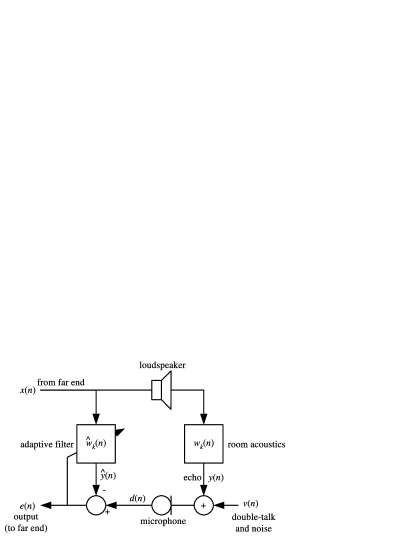
Figure 1: Block diagram of echo cancellation system

The complex NLMS filter (Fig. 1) of length $N$ is defined as:

$$e(n)=d(n)-\hat{y}(n)=d(n)-\sum_{k=0}^{N-1}\hat{w}_{k}(n)x(n-k)$$ (1)

with adaptation step [6]:

$$\!\!\!\!\!\!\hat{w}_{k}\!(\!n\!+\!1\!) \!\!\!\!= \!\!\!\!\hat{w}_{k}(n)\!+\!\mu\frac{e(n)x^{*}(n-k)}{\sum_{i=0}^{N-1}\left|x(n-i)\right|^{2}}$$ (2)

$$\!\!\!\!= \!\!\!\!\hat{w}_{k}(n)\!+\!\mu\frac{\left(d(n)\!-\!\sum_{i}\!\!\hat{w}_{i}(n)x(n\!-\!i)\!\right)\!x^{*}(n\!-\!k)}{\sum_{i=0}^{N-1}\left|x(n-i)\right|^{2}}$$ (3)

where $x(n)$ is the far-end signal, $\hat{w}_{k}(n)$ are the estimated filter weights at time $n$ and $\mu$ is the learning rate.

Considering the error on the filter weights $\delta_{k}(n)=\hat{w}_{k}(n)-w_{k}(n)$, and knowing $d(n)=v(n)+\sum_{k}w_{k}(n)x(n-k)$, then (3) can be re-written as:

$$\delta_{k}(n+1)\!=\!\delta_{k}(n)+\mu\frac{\left(v(n)-\sum_{i}\!\delta_{i}(n)x(n\!-\!i)\right)x^{*}(n\!-\!k)}{\sum_{i=0}^{N-1}\left|x(n-i)\right|^{2}}$$ (4)

At each time step, the filter misadjustment $\Lambda(n)=\sum_{k}\delta_{k}^{*}(n)\delta_{k}(n)$ can be obtained as:

$$\Lambda(\!n\!+\!1\!)\!=\!\sum_{k=0}^{N-1}\left|\delta_{k}(n)\!+\!\mu\frac{\!\left(\!v(n)-\sum_{i}\!\delta_{i}(n)x(\!n\!-\!i)\right)x^{*}(\!n\!-\!k)}{\sum_{i=0}^{N-1}\left|x(n-i)\right|^{2}}\!\right|^{2}$$ (5)

By making the (strong) assumption that $x(n)$ and $v(n)$ are white noise signals uncorrelated to each other, we find that:

$$\footnotesize{E\!\left\{\Lambda(n+1)|\Lambda(n),\!x(n)\right\}\!=\!\Lambda(n)\!\!\left[\!1\!-\!\frac{2\mu}{N}\!+\!\frac{\mu^{2}}{N}\!+\!\frac{\mu^{2}\sigma_{v}^{2}}{\Lambda(n)\!\!\sum_{i=0}^{N-1}\!\!\left|x(n-i)\right|^{2}}\!\right]}$$ (6)

where the expectation operator $E\left\{\cdot\right\}$ is only taken over $v(n)$ at this point and $\sigma_{v}^{2}=E\left\{\left|v(n)\right|^{2}\right\}$. Because (6) is a convex function, the expected misadjustment can be minimized with respect to $\mu$ by solving $\partial E\left\{\Lambda(n+1)\right\}/\partial\mu=0$ with $\Lambda(n)\neq 0$:

$$\frac{-2}{N}+\frac{2\mu}{N}+\frac{2\mu\sigma_{v}^{2}}{\Lambda(n)\sum_{i=0}^{N-1}\left|x(n-i)\right|^{2}}=0$$ (7)

This leads to the conditional optimal learning rate (conditioned on the current misadjustment and the far-end signal):

$$\mu_{opt}(n)=\frac{1}{1+\frac{\sigma_{v}^{2}}{\Lambda(n)(1/N)\sum_{i=0}^{N-1}\left|x(n-i)\right|^{2}}}$$ (8)

When there is no near-end noise ($\sigma_{v}^{2}$), we can see that (8) simplifies to $\mu_{opt}(n)=1$, which is consistent with [7]. Now, considering that the expectation of $\Lambda(n)\sum_{i=0}^{N-1}\left|x(n-i)\right|^{2}/N$ over $x(n)$ is equal to the variance $\sigma_{r}^{2}(n)$ of the residual echo $r(n)=y(n)-\hat{y}(n)$, and knowing that the output signal variance is $\sigma_{e}^{2}(n)=\sigma_{v}^{2}(n)+\sigma_{r}^{2}(n)$, we approximate (the approximation becomes exact as $N$ goes to infinity) the optimal learning rate as:

$$\mu_{opt}(n)\approx\frac{\sigma_{r}^{2}(n)}{\sigma_{e}^{2}(n)}$$ (9)

This means that the optimal learning rate is approximately proportional to the residual-to-error ratio. Note that $\sigma_{e}^{2}(n)$ can easily be estimated, however the estimation of the residual echo $\sigma_{r}^{2}(n)$ is difficult and addressed in the next section. For now if we assume we have the estimates $\hat{\sigma}_{r}^{2}(n)$ and $\hat{\sigma}_{e}^{2}(n)$ we can choose the learning rate as:

$$\hat{\mu}_{opt}(n)=\min\left(\frac{\hat{\sigma}_{r}^{2}(n)}{\hat{\sigma}_{e}^{2}(n)},1\right)$$ (10)

where the upper bound is the optimal rate for the noiseless case and reflects the fact that $\sigma_{e}^{2}(n)$ is always greater than $\sigma_{r}^{2}(n)$.

Another result that can be obtained from (6) is that the adaptation of the filter will stall ($E\left\{\Lambda(n+1)\right\}=\Lambda(n)$) when:

$$\Lambda(n)\approx\frac{\sigma_{v}^{2}}{\sigma_{x}^{2}\left(\frac{2}{\mu}-1\right)}$$ (11)

where $\sigma_{x}^{2}$ is the variance of the filter input (far end) signal. Substituting the value of $\hat{\mu}_{opt}$ in (10) into (11), we obtain that upon a stall in the filter adaptation, the residual echo is:

$$\sigma_{r}^{2}(n)\approx\min\left(\frac{1}{2}\hat{\sigma}_{r}^{2}(n),\sigma_{v}^{2}(n)\right)$$ (12)

where the first argument of the $\min\left(\cdot\right)$ is obtained by solving

$$\sigma_{r}^{2}(n)=\frac{\sigma_{v}^{2}(n)}{\frac{2\left(\sigma_{r}^{2}(n)+\sigma_{v}^{2}(n)\right)}{\hat{\sigma}_{r}^{2}(n)}-1}$$ (13)

The result in (12) means that the residual echo is bounded by the background noise and by half of the estimated residual echo, whichever is lower. For this reason, it is important not to overestimate the residual echo by more than 3 dB, at least during double-talk.

III Application to the MDF Algorithm With Background Noise and Double-Talk

The derivation in Section II makes the assumption that $x(n)$ and $v(n)$ are white noise signals. While the assumption obviously does not hold in the case of acoustic echo cancellation of speech signals using the NLMS algorithm, we propose to apply it to adaptive filter algorithms that operate in the frequency domain. In this section, we concentrate on the multidelay block frequency domain (MDF) adaptive filter [3]. The adaptation used for the MDF algorithm (and other block frequency algorithms) is similar to applying NLMS algorithm independently for each frequency. It has been observed that the input signals are less correlated in time (across consecutive FFT frames) than the original time-domain signal. Also, the learning rate $\mu(k,\ell)$ can be made frequency-dependent. In this section, variables $\hat{Y}(k,\ell)$ and $E(k,\ell)$ are the frequency-domain counterparts of $\hat{y}(n)$ and $e(n)$, where $k$ is the frequency index and $\ell$ is the frame index.

Assuming the signals for each frequency of the MDF algorithm are uncorrelated in time, we approximate the optimal frequency-dependent learning rate by:

$$\mu_{opt}(k,\ell)\approx\frac{\sigma_{r}^{2}(k,\ell)}{\sigma_{e}^{2}(k,\ell)}$$ (14)

where $k$ is the discrete frequency and $\ell$ is the frame index. In order to estimate the residual echo $\sigma_{r}^{2}(k,\ell)$, we make the assumption that the adaptive filter has a frequency-independent leakage coefficient $\eta(\ell)$ that represents the misadjustment of the filter. This leads to the estimate:

$$\hat{\sigma}_{r}^{2}(k,\ell)=\hat{\eta}(\ell)\hat{\sigma}_{\hat{Y}}^{2}(k,\ell)$$ (15)

where $\hat{\eta}(\ell)$ is the estimate leakage coefficient. The advantage of this formulation is that it factors the residual estimation $\sigma_{r}^{2}(k,\ell)$ into a slowly-evolving, but difficult to estimate term ($\hat{\eta}(\ell)$) and a rapidly-evolving, but easy to estimate term ($\hat{\sigma}_{\hat{Y}}^{2}(k,\ell)$). The leakage coefficient $\eta(\ell)$ is in fact the inverse of the echo return loss enhancement (ERLE) of the filter.

It is desirable for the learning rate to have a fast response in the case of double-talk in order to prevent the filter from diverging when double-talk starts. For this reason, we use the instantaneous estimations $\hat{\sigma}_{y}(k,\ell)=\left|Y(k,\ell)\right|^{2}$ and $\hat{\sigma}_{e}(k,\ell)=\left|E(k,\ell)\right|^{2}$. Based on (10), this leads to the learning rate:

$$\hat{\mu}_{opt}(k,\ell)=\min\left(\hat{\eta}(\ell)\frac{\left|\hat{Y}(k,\ell)\right|^{2}}{\left|E(k,\ell)\right|^{2}},\>\mu_{max}\right)$$ (16)

where $\mu_{max}$ is a design parameter (always less than or equal to 1) which puts a ceiling on the learning rate for practical purposes and ensures that the learning rate cannot cause the adaptive filter to become unstable.

We see from (16) that the effects of the filter misadjustment and the double-talk are decoupled. The learning rate can thus react quickly to double-talk even if the estimation of the residual echo (leakage coefficient) requires a longer time period.

An important aspect that needs to be addressed is the initial condition. When the filter is initialized, all the weights are set to zero, so the $Y(k,\ell)$ signal is also zero. This causes the learning rate computed using (16) to be zero. In order to start the adaptation process, the learning rate $\mu(k,\ell)$ is set to a fixed constant (we use $\mu(k,\ell)=0.25$) for a short time equal to twice the filter length (only non-zero portions of signal $x(n)$ are taken into account). This procedure is only necessary when the filter is initialized and is not required in case of echo path change.

III-A Leakage estimation

We see from (16) that the optimal learning rate depends heavily the estimated leakage coefficient $\hat{\eta}(\ell)$. We propose to estimate the leakage coefficient $\eta(\ell)$ by exploiting the non-stationarity of the signals and using linear regression between the power spectra of the estimated echo and the output signal. This choice is based on the fact that the spectrum of the residual echo is highly correlated with that of the estimated echo, while there is no correlation between the spectrum of the echo and that of the noise.

First, a zero-mean version of the power spectra is obtained using a first order DC rejection filter:

$$P_{Y}(k,\ell) = (1-\gamma)P_{Y}(k,\ell-1)$$ (17)

$$+\gamma\left(\left|\hat{Y}(k,\ell)\right|^{2}-\left|\hat{Y}(k,\ell-1)\right|^{2}\right)$$

$$P_{E}(k,\ell) = (1-\gamma)P_{E}(k,\ell-1)$$ (18)

$$+\gamma\left(\left|E(k,\ell)\right|^{2}-\left|E(k,\ell-1)\right|^{2}\right)$$

From there, $\hat{\eta}(\ell)$ is equal to the linear regression coefficient between the estimated echo power $P_{Y}(k,\ell)$ and output power $P_{E}(k,\ell)$:

$$\hat{\eta}(\ell)=\frac{\sum_{k}R_{EY}(k,\ell)}{\sum_{k}R_{YY}(k,\ell)}$$ (19)

where the correlations $R_{EY}(k,\ell)$ and $R_{YY}(k,\ell)$ are averaged recursively as:

$$\!\!\!\!R_{EY}(k,\ell) \!\!\!\!\!= \!\!\!\!\!(1\!-\!\beta(\ell))R_{EY}(k,\ell)+\beta(\ell)P_{Y}(k)P_{E}(k)$$ (20)

$$\!\!\!\!R_{YY}(k,\ell) \!\!\!\!\!= \!\!\!\!\!(1\!-\!\beta(\ell))R_{YY}(k,\ell)+\beta(\ell)\left(P_{Y}(k)\right)^{2}$$ (21)

$$\!\!\!\!\beta(\ell) \!\!\!\!\!= \!\!\!\!\!\beta_{0}\min\left(\frac{\hat{\sigma}_{\hat{Y}}^{2}(\ell)}{\hat{\sigma}_{e}^{2}(\ell)},1\right)$$ (22)

$\beta_{o}$ is the base learning rate for the leakage estimate and $\hat{\sigma}_{\hat{Y}}^{2}(\ell)$ and $\hat{\sigma}_{\hat{e}}^{2}(\ell)$ are respectively the total power of the estimated echo and the output signal. The variable averaging parameter $\beta(\ell)$ prevents the estimate from being adapted when no echo is present.

III-B Double-talk, background noise and echo path change

It can be seen that the adaptive learning rate described above is able to deal with both double-talk and echo path change without explicit modelling. From (16) we can see that when double-talk occurs, the denominator $\left|E(k,\ell)\right|^{2}$ rapidly increases, causing an instantaneous decrease in the learning rate that lasts only as long as the double-talk period lasts. In the case of background noise, the learning rate depends on both the presence of an echo signal as well as the leakage estimate. As the filter misadjustment becomes smaller, the learning rate will also become smaller.

One major difficulty involved in double-talk detection is the need to distinguish between double-talk and echo path change, both of which causing a sudden increase in the filter error signal. This distinction is done by the leakage estimate. In conditions of double-talk, there is little correlation between the power spectrum of the error and that of the estimated echo, so $\hat{\eta}(\ell)$ remains small and so does the learning rate. On the other hand, when the echo path changes, there is a large correlation between the power spectra, which leads to a rapid increase of $\hat{\eta}(\ell)$ that can quickly bring the learning rate close to unity if the change is large and there is no double-talk.

IV Results And Discussion

The proposed system is evaluated in an acoustic echo cancellation context with background noise, double-talk and a change in the echo path. The two different impulse responses used are 1024-sample long and measured from real recordings in a small office with both the microphone and the loudspeaker resting on a desk.

The proposed algorithm is compared to the Gänsler double-talk detector [1], to the normalized cross-correlation method [2] and to a baseline with no double-talk detection (no DTD). In the implementation of the Gänsler algorithm, the delay estimation is performed off-line and the coherence threshold is set to 0.3, since that value was found to be optimal for the present case. We would expect the performance of the Gänsler algorithm to degrade if automatic estimation of these parameters were to be used. The optimal threshold found for the normalization algorithm was also 0.3. It was found that choosing $\mu_{max}=0.5$ as the upper bound on the learning rate gave good results for our algorithm. In practice, finding $\mu_{max}$ is not hard, since the algorithm is not very sensitive to that parameter. For the other algorithms tested, best results were achieved using $\mu=0.2$ as the learning rate.

For a typical 32-second scenario, the signals for the near-end and far-end are shown in Fig. 2a), with The echo path changing after 16 seconds. The measured echo return loss enhancement (ERLE) is shown in Fig. 2b) for all algorithms. Because of natural variations in the behavior of the algorithms, it is not immediately possible to determine the most accurate algorithm from this plot. However, we show it here to demonstrate the behavior of our algorithm. For example, it can be observed that when the echo path changes after 16 seconds, the proposed algorithm re-adapts faster than the other algorithms with double-talk detection and almost as fast as the echo canceller without double-talk detection.

Figure 2: (a) Convolved far end signal $y(n)$ (top), near end signal $v(n)$ (middle), captured signal $d(n)$ (bottom). (b) Short-term ERLE as a function of time. Gaps in the curves are due to the fact that the ERLE is undefined when the far-end signal is zero.

The estimate of the ERLE (computed as $1/\hat{\eta}(\ell)$) is provided in Fig. 3. It can be observed that the estimate roughly follows the measured ERLE, although the estimation is obviously noisy. Most importantly, it almost never overestimates the residual echo (underestimate ERLE) by more than 3 dB, as is required by (12). Also, when the echo path changes, the estimate rapidly falls toward 0 dB, which is the desired behavior. Fig. 4 shows how the learning rate varies as a function of time for all three algorithms. The effect of the leakage estimation can be clearly observed when the learning rate rapidly goes up after the echo path change at $t=16\>s$, remaining well above the learning rate of the other algorithms for about 5 seconds. It is also observed that the learning rate goes down as the filter becomes better adapted. This is an advantage over the Gänsler and normalized cross-correlation algorithms that do not take into account the filter misadjustment.

Figure 3: Echo Return Loss Enhancement (ERLE) estimate, computed as the inverse of estimated leakage coefficient ($1/\hat{\eta}(\ell)$), compared to the measured ERLE.

Figure 4: Learning rate averaged over a 600 ms moving window for all three algorithms. For the proposed algorithm, the learning rate is also averaged over all frequencies. The learning rate for the Gänsler and normalized cross-correlation algorithms appear to to have a continuous scale only due to the time averaging. The learning rate sometimes goes to zero when there is no far-end signal.

Fig. 5 shows the average steady-state (the first 2 seconds of adaptation are not considered) ERLE for the data of Fig. 2 with different ratios of near-end signal and echo. Clearly, the proposed algorithm performs better than both the Gänsler and normalized cross-correlation algorithms in all cases, with an average improvement of more than 4 dB in both cases. The perceptual quality of the output speech signal is also evaluated by comparing it to the near field signal $v(n)$ using the Perceptual Evaluation of Speech Quality (PESQ) ITU-T recommendations P.862 [8] and P.862.1 [9]. The perceptual quality of the speech shown in Fig. 6 is evaluated based on the entire file, including the adaptation time. It is again clear that the proposed algorithm performs better than the reference double-talk detectors. It is worth noting that the reason why the results in Fig. 5 improve with double-talk (unlike in Fig. 5) is that the signal of interest is the double-talk $v(n)$, so the higher the double-talk the less (relative) echo in the input signal.

Figure 5: Steady-state ERLE (first two seconds of adaptation not considered) as a function of the v-to-y signal ratio ($20\log_{10}(\sigma_{v}^{2}/\sigma_{y}^{2})$). The filter fails to converge in the “no DTD” case when the ratio is equal or above 10 dB.

Figure 6: PESQ objective listening quality measure (LQO-MOS) as a function of the v-to-y signal ratio ($20\log_{10}(\sigma_{v}^{2}/\sigma_{y}^{2})$). The filter fails to improve in the “no DTD” case when the ratio is equal or above 10 dB.

V Conclusion

We have demonstrated a novel method for adjusting the learning rate of frequency-domain adaptive filters based on the current misadjustment and the amount of noise and double-talk present. The proposed method performs better than a coherence-based double-talk detector, does not use a hard detection threshold and does not require explicit estimation of the echo path delay. While the demonstration is done using the MDF algorithm, we believe the technique is general enough and applicable to other frequency-domain adaptive filtering algorithms.

In future work, the residual echo estimation in (15) could be evaluated as a residual echo estimator for further suppression of the echo, as proposed in [10]. Also, more accurate methods for estimating the leakage coefficient should be researched.

Jean-Marc Valin (S’03-M’05) was born in Montreal, Canada in 1976. He received his B.Eng. degree, M.Sc. degree and Ph.D. in the electrical engineering from the University of Sherbrooke in 1999, 2001 and 2005 respectively. His Ph.D. research focused on bringing auditory capabilities to a mobile robotics platform, including sound source localization and separation. Since 2005, he is a post-doctoral fellow at the CSIRO ICT Centre in Sydney, Australia. His research topics include acoustic echo cancellation and microphone array processing. He is the author of the Speex speech codec.

References

- [1] T. Gänsler, M. Hansson, C.-J. Ivarsson, and G. Salomonsson, “A double-talk detector based on coherence,” IEEE Transactions on Communications, vol. 44, no. 11, pp. 1421–1427, 1996.
- [2] J. Benesty, D. Morgan, and J. Cho, “A new class of doubletalk detectors based on cross-correlation,” IEEE Transactions on Speech and Audio Processing, vol. 8, no. 2, pp. 168–172, 2000.
- [3] J.-S. Soo and K. Pang, “Multidelay block frequency domain adaptive filter,” IEEE Transactions on Acoustics, Speech and Signal Processing, vol. 38, no. 2, pp. 373–376, 1990.
- [4] W.-P. Ang and B. Farhang-Boroujeny, “A new class of gradient adaptive step-size lms algorithms,” IEEE Transactions on Signal Processing, vol. 49, no. 4, pp. 805–810, 2001.
- [5] D. Mandic, “A generalized normalized gradient descent algorithm,” IEEE Signal Processing Letters, vol. 11, no. 2, pp. 115–118, 2004.
- [6] S. Haykin, Adaptive Filter Theory. Prentice Hall, 4 ed., 2002.
- [7] T. Hsia, “Convergence analysis of LMS and NLMS adaptive algorithms,” in Proceedings IEEE International Conference on Acoustics, Speech, and Signal Processing, vol. 8, pp. 667–670, 1983.
- [8] ITU-T, Perceptual evaluation of speech quality (PESQ): An objective method for end-to-end speech quality assessment of narrow-band telephone networks and speech codecs. International Telecommunications Union, 2001.
- [9] ITU-T, Mapping function for transforming P.862 raw result scores to MOS-LQO. International Telecommunications Union, 2003.
- [10] S. Gustafsson, R. Martin, P. Jax, and P. Vary, “A psychoacoustic approach to combined acoustic echo cancellation and noise reduction,” IEEE Transactions on Speech and Audio Processing, vol. 10, no. 5, pp. 245–256, 2002.