Abstract

For the search for additional Higgs bosons in the Minimal Supersymmetric Standard Model (MSSM) as well as for future precision analyses in the Higgs sector a precise knowledge of their production properties is mandatory. We review the evaluation of the cross sections for the neutral Higgs boson production at $e^{+}e^{-}$ linear colliders in the MSSM with complex parameters (cMSSM). The evaluation is based on a full one-loop calculation of the production mechanism $e^{+}e^{-}\to h_{i}Z,\,h_{i}\gamma,\,h_{i}h_{j}$ $(i,j=1,2,3)$, including soft and hard QED radiation. The dependence of the Higgs boson production cross sections on the relevant cMSSM parameters is analyzed numerically. We find sizable contributions to many cross sections. They are, depending on the production channel, roughly of 10-20% of the tree-level results, but can go up to 50% or higher.

1 Introduction

The most frequently studied models for electroweak symmetry breaking are the Higgs mechanism within the Standard Model (SM) and within the Minimal Supersymmetric Standard Model (MSSM) [1, 2, 3]. Contrary to the case of the SM, in the MSSM two Higgs doublets are required. This results in five physical Higgs bosons instead of the single Higgs boson in the SM. In lowest order these are the light and heavy ${\cal CP}$-even Higgs bosons, $h$ and $H$, the ${\cal CP}$-odd Higgs boson, $A$, and two charged Higgs bosons, $H^{\pm}$. Within the MSSM with complex parameters (cMSSM), taking higher-order corrections into account, the three neutral Higgs bosons mix and result in the states $h_{i}$ ($i=1,2,3$) [4, 5, 6, 7]. The Higgs sector of the cMSSM is described at the tree-level by two parameters: the mass of the charged Higgs boson, $M_{H^{\pm}}$, and the ratio of the two vacuum expectation values, $\tan\beta\equiv t_{\beta}=v_{2}/v_{1}$. Often the lightest Higgs boson, $h_{1}$ is identified [8] with the particle discovered at the LHC [9, 10] with a mass around $\sim 125\,\,\mathrm{GeV}$ [11].

If supersymmetry (SUSY) is realized in nature the additional Higgs bosons could be produced at a future linear $e^{+}e^{-}$ collider such as the ILC [12, 13, 14, 15] or CLIC [16, 15]. In the case of a discovery of additional Higgs bosons a subsequent precision measurement of their properties will be crucial to determine their nature and the underlying (SUSY) parameters. In order to yield a sufficient accuracy, one-loop corrections to the various Higgs boson production and decay modes have to be considered. Full one-loop calculations in the cMSSM for various Higgs boson decays to SM fermions, scalar fermions and charginos/neutralinos have been presented over the last years [17, 18, 19]. For the decay to SM fermions see also Refs. [20, 21, 22]. Decays to (lighter) Higgs bosons have been evaluated at the full one-loop level in the cMSSM in Ref. [17]; see also Refs. [23, 24]. Decays to SM gauge bosons (see also Ref. [25]) can be evaluated to a very high precision using the full SM one-loop result [26] combined with the appropriate effective couplings [27]. The full one-loop corrections in the cMSSM listed here together with resummed SUSY corrections have been implemented into the code FeynHiggs [28, 29, 30, 27, 31].

Particularly relevant are higher-order corrections also for the Higgs boson production at $e^{+}e^{-}$ colliders, where a very high accuracy in the Higgs property determination is anticipated [15]. Here we review the calculation of the neutral Higgs boson production at $e^{+}e^{-}$ colliders in association with a SM gauge boson or another cMSSM Higgs boson as presented in [32],

$$\sigma(e^{+}e^{-}\to h_{i}h_{j})\,,$$ (1)

$$\sigma(e^{+}e^{-}\to h_{i}Z)\,,$$ (2)

$$\sigma(e^{+}e^{-}\to h_{i}\gamma)\,.$$ (3)

The processes $e^{+}e^{-}\to h_{i}h_{i}$ and $e^{+}e^{-}\to h_{i}\gamma$ are purely loop-induced.

The results reviewed here consist of a full one-loop calculation Taken into account are soft and hard QED radiation, collinear divergences and the $\hat{Z}$ factor contributions. In this way we go substantially beyond the existing calculations in the literature, see Ref. [32] for details.

Here we will concentrate on examples for the numerical results. Details on the renormalization of the cMSSM, the evaluation of the loop diagrams, the cancellation of UV, IR and collinear divergences, as well as a comparison with previous, less advanced calculations can be found in Ref. [32].

2 Numerical Examples

Here we review examples for the numerical analysis of neutral Higgs boson production at the ILC or CLIC. In the various figures below we show the cross sections at the tree-level (“tree”) and at the full one-loop level (“full”). In case of extremely small tree-level cross sections we also show results including the corresponding purely loop induced contributions (“loop”). These leading two-loop contributions are $\propto|{\cal M}_{\text{1-loop}}|^{2}$, where ${\cal M}_{\text{1-loop}}$ denotes the one-loop matrix element of the appropriate process.

2.1 Parameter settings

Details on the SM parameters can be found in Ref. [32]. The Higgs sector quantities (masses, mixings, $\hat{Z}$ factors, etc.) have been evaluated using FeynHiggs (version 2.11.0) [28, 29, 30, 27, 31]. The SUSY parameters are chosen according to the scenario $\mathcal{S}$, shown in Tab. 1, unless otherwise noted. This scenario constitutes a viable scenario for the various cMSSM Higgs production modes, i.e. not picking specific parameters for each cross section. the only variation will be the choice of $\sqrt{s}=500\,\,\mathrm{GeV}$ for production cross sections involving the light Higgs boson.

Table 1: MSSM default parameters for the numerical investigation; all parameters (except of $t_{\beta}$) are in GeV (calculated masses are rounded to 1 MeV). the values for the trilinear sfermion Higgs couplings, $A_{t,b,\tau}$ are chosen such that charge- and/or color-breaking minima are avoided [33], and $A_{b,\tau}$ are chosen to be real. It should be noted that for the first and second generation of sfermions we chose instead $A_{f}=0$, $M_{\tilde{Q},\tilde{U},\tilde{D}}=1500\,\,\mathrm{GeV}$ and $M_{\tilde{L},\tilde{E}}=500\,\,\mathrm{GeV}$.

Scen.	$\sqrt{s}$	$t_{\beta}$	$\mu$	$M_{H^{\pm}}$	$M_{\tilde{Q},\tilde{U},\tilde{D}}$	$M_{\tilde{L},\tilde{E}}$	$|A_{t,b,\tau}|$	$M_{1}$	$M_{2}$	$M_{3}$
$\mathcal{S}$	1000	7	200	300	1000	500	$1500+\mu/t_{\beta}$	100	200	1500

$m_{h_{1}}$	$m_{h_{2}}$	$m_{h_{3}}$
123.404	288.762	290.588

The numerical results shown in the next subsections are of course dependent on the choice of the SUSY parameters. Nevertheless, they give an idea of the relevance of the full one-loop corrections.

2.2 The process $e^{+}e^{-}\to h_{i}h_{j}$

We start our analysis with the production modes $e^{+}e^{-}\to h_{i}h_{j}$ ($i,j=1,2$). Results are shown in the Figs. 1, 2. We begin with the process $e^{+}e^{-}\to h_{1}h_{2}$ as shown in Fig. 1. As a general comment it should be noted that in $\mathcal{S}$ one finds that $h_{1}\sim h$, $h_{2}\sim A$ and $h_{3}\sim H$. the $hAZ$ coupling is $\propto c_{\beta-\alpha}$ which goes to zero in the decoupling limit [34], and consequently relatively small cross sections are found. In the analysis of the production cross section as a function of $\sqrt{s}$ (upper left plot) we find the expected behavior: a strong rise close to the production threshold, followed by a decrease with increasing $\sqrt{s}$. We find a relative correction of $\sim-15\%$ around the production threshold. Away from the production threshold, loop corrections of $\sim+27\%$ at $\sqrt{s}=1000\,\,\mathrm{GeV}$ are found in $\mathcal{S}$ (see Tab. 1). the relative size of loop corrections increase with increasing $\sqrt{s}$ and reach $\sim+61\%$ at $\sqrt{s}=3000\,\,\mathrm{GeV}$ where the tree-level becomes very small.

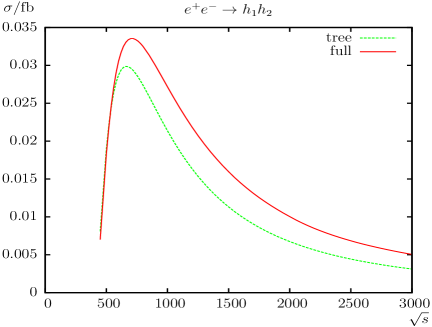
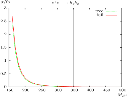
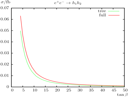
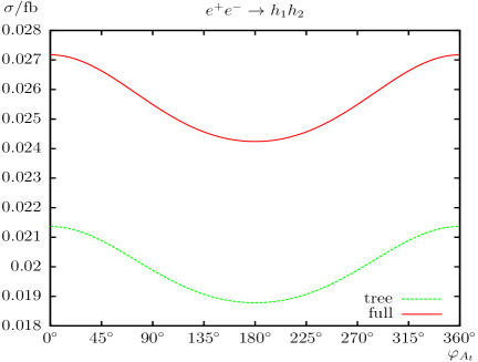
Figure 1: $\sigma(e^{+}e^{-}\to h_{1}h_{2})$. Tree-level and full one-loop corrected cross sections are shown with parameters chosen according to $\mathcal{S}$; see Tab. 1. the upper plots show the cross sections with $\sqrt{s}$ (left) and $M_{H^{\pm}}$ (right) varied; the lower plots show $t_{\beta}$ (left) and $\varphi_{A_{t}}$ (right) varied.

With increasing $M_{H^{\pm}}$ in $\mathcal{S}$ (upper right plot) we find a strong decrease of the production cross section, as can be expected from kinematics, but in particular from the decoupling limit discussed above. The loop corrections reach $\sim+27\%$ at $M_{H^{\pm}}=300\,\,\mathrm{GeV}$ and $\sim+62\%$ at $M_{H^{\pm}}=500\,\,\mathrm{GeV}$. These large loop corrections are again due to the (relative) smallness of the tree-level results. It should be noted that at $M_{H^{\pm}}\approx 350\,\,\mathrm{GeV}$ the limit of $0.01$ fb is reached, corresponding to 10 events at an integrated luminosity of ${\cal L}=1\,\mbox{ab}^{-1}$. The cross sections decrease with increasing $t_{\beta}$ (lower left plot), and the loop corrections reach the maximum of $\sim+38\%$ at $t_{\beta}=36$ while the minimum of $\sim+26\%$ is at $t_{\beta}=5$. The phase dependence $\varphi_{A_{t}}$ of the cross section in $\mathcal{S}$ (lower right plot) is at the 10% level at tree-level. The loop corrections are nearly constant, $\sim+28\%$ for all $\varphi_{A_{t}}$ values and do not change the overall dependence of the cross section on the complex phase.

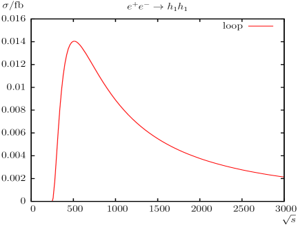
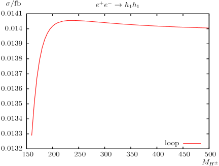
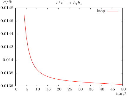
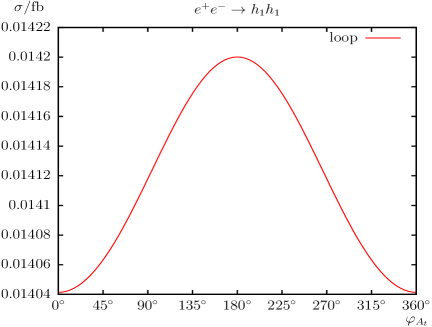
Figure 2: $\sigma(e^{+}e^{-}\to h_{1}h_{1})$. Loop induced (i.e. leading two-loop corrected) cross sections are shown with parameters chosen according to $\mathcal{S}$ (see Tab. 1), but with $\sqrt{s}=500\,\,\mathrm{GeV}$. the upper plots show the cross sections with $\sqrt{s}$ (left) and $M_{H^{\pm}}$ (right) varied; the lower plots show $t_{\beta}$ (left) and $\varphi_{A_{t}}$ (right) varied.

We now turn to the processes with equal indices. the tree couplings $h_{i}h_{i}Z$ ($i=1,2,3$) are exactly zero; see Ref. [35]. Therefore, in this case we show the pure loop induced cross sections $\propto|{\cal M}_{\text{1-loop}}|^{2}$ (labeled as “loop”) where only the box diagrams contribute. These box diagrams are UV and IR finite.

In Fig. 2 we show the results for $e^{+}e^{-}\to h_{1}h_{1}$. This process might have some special interest, since it is the lowest energy process in which triple Higgs boson couplings play a role, which could be relevant at a high-luminosity collider operating above the two Higgs boson production threshold. In our numerical analysis, as a function of $\sqrt{s}$ we find a maximum of $\sim 0.014$ fb, at $\sqrt{s}=500\,\,\mathrm{GeV}$, decreasing to $\sim 0.002$ fb at $\sqrt{s}=3\,\,\mathrm{TeV}$. The dependence on $M_{H^{\pm}}$ is rather small, as is the dependence on $t_{\beta}$ and $\varphi_{A_{t}}$ in $\mathcal{S}$. However, with cross sections found at the level of up to $0.015$ fb this process could potentially be observable at the ILC running at $\sqrt{s}=500\,\,\mathrm{GeV}$ or below (depending on the integrated luminosity).

2.3 The process $e^{+}e^{-}\to h_{i}Z$

In Figs. 3 and 4 we show the results for the processes $e^{+}e^{-}\to h_{i}Z$ ($i=1,3$), as before as a function of $\sqrt{s}$, $M_{H^{\pm}}$, $t_{\beta}$ and $\varphi_{A_{t}}$. It should be noted that there are no $AZZ$ couplings in the MSSM (see [35]). In the case of real parameters this leads to vanishing tree-level cross sections if $h_{i}\sim A$.

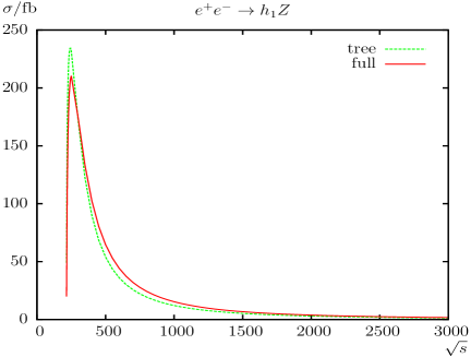
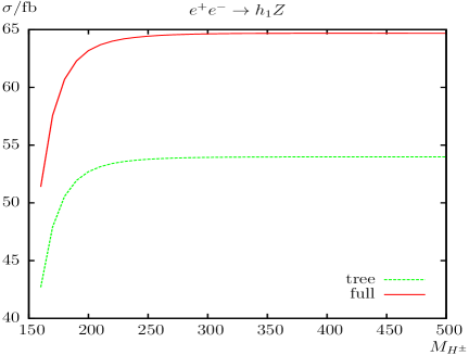
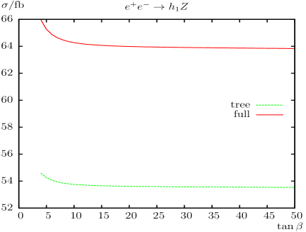
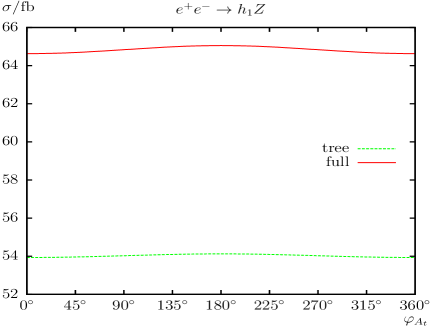
Figure 3: $\sigma(e^{+}e^{-}\to h_{1}Z)$. Tree-level and full one-loop corrected cross sections are shown with parameters chosen according to $\mathcal{S}$ (see Tab. 1), but with $\sqrt{s}=500\,\,\mathrm{GeV}$. the upper plots show the cross sections with $\sqrt{s}$ (left) and $M_{H^{\pm}}$ (right) varied; the lower plots show $t_{\beta}$ (left) and $\varphi_{A_{t}}$ (right) varied.

We start with the process $e^{+}e^{-}\to h_{1}Z$ shown in Fig. 3. In $\mathcal{S}$ one finds $h_{1}\sim h$, and since the $ZZh$ coupling is $\propto s_{\beta-\alpha}\to 1$ in the decoupling limit, relative large cross sections are found. As a function of $\sqrt{s}$ (upper left plot) a maximum of more than $200$ fb is found at $\sqrt{s}\sim 250\,\,\mathrm{GeV}$ with a decrease for increasing $\sqrt{s}$. The size of the corrections of the cross section can be especially large very close to the production threshold from which on the considered process is kinematically possible. At the production threshold we found relative corrections of $\sim-60\%$. Away from the production threshold, loop corrections of $\sim+20\%$ at $\sqrt{s}=500\,\,\mathrm{GeV}$ are found, increasing to $\sim+30\%$ at $\sqrt{s}=3000\,\,\mathrm{GeV}$. In the following plots we assume, deviating from the definition of $\mathcal{S}$, $\sqrt{s}=500\,\,\mathrm{GeV}$.

As a function of $M_{H^{\pm}}$ (upper right plot) the cross sections strongly increases up to $M_{H^{\pm}}\;\raisebox{-3.00003pt}{$\stackrel{{\scriptstyle\displaystyle<}}{{\sim}}$}\;250\,\,\mathrm{GeV}$, corresponding to $s_{\beta-\alpha}\to 1$ in the decoupling limit discussed above. For higher $M_{H^{\pm}}$ values it is nearly constant, and the loop corrections are $\sim+20\%$ for $160\,\,\mathrm{GeV}<M_{H^{\pm}}<500\,\,\mathrm{GeV}$. Hardly any variation is found for the production cross section as a function of $t_{\beta}$ or $\varphi_{A_{t}}$. In both cases the one-loop corrections are found at the level of $\sim+20\%$.

Not shown is the process $e^{+}e^{-}\to h_{2}Z$, which turns out to be very small in our scenario $\mathcal{S}$. We finish the $e^{+}e^{-}\to h_{i}Z$ analysis in Fig. 4 in which the results for $e^{+}e^{-}\to h_{3}Z$ are shown. In $\mathcal{S}$ one has $h_{3}\sim H$, and with the $ZZH$ coupling being proportional to $c_{\beta-\alpha}\to 0$ in the decoupling limit relatively small production cross sections are found for $M_{H^{\pm}}$ not too small.

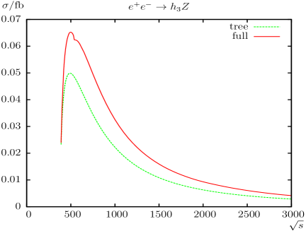
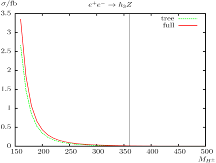
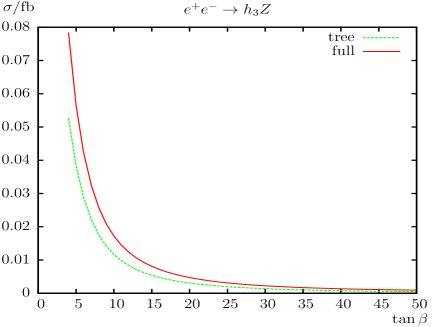
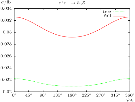
Figure 4: $\sigma(e^{+}e^{-}\to h_{3}Z)$. Tree-level and full one-loop corrected cross sections are shown with parameters chosen according to $\mathcal{S}$; see Tab. 1. the upper plots show the cross sections with $\sqrt{s}$ (left) and $M_{H^{\pm}}$ (right) varied; the lower plots show $t_{\beta}$ (left) and $\varphi_{A_{t}}$ (right) varied.

As a function of $\sqrt{s}$ (upper left plot) a dip can be seen at $\sqrt{s}\approx 540\,\,\mathrm{GeV}$, due to the threshold $m_{\tilde{\chi}_{2}^{\pm}}+m_{\tilde{\chi}_{2}^{\pm}}=\sqrt{s}$. Around the production threshold we found relative corrections of $\sim 3\%$. the maximum production cross section is found at $\sqrt{s}\sim 500\,\,\mathrm{GeV}$ of about $0.065$ fb including loop corrections, rendering this process observable with an accumulated luminosity ${\cal L}\;\raisebox{-3.00003pt}{$\stackrel{{\scriptstyle\displaystyle<}}{{\sim}}$}\;1\,\mbox{ab}^{-1}$. Away from the production threshold, one-loop corrections of $\sim 47\%$ at $\sqrt{s}=1000\,\,\mathrm{GeV}$ are found in $\mathcal{S}$ (see Tab. 1), with a cross section of about $0.03$ fb. the cross section further decreases with increasing $\sqrt{s}$ and the loop corrections reach $\sim 45\%$ at $\sqrt{s}=3000\,\,\mathrm{GeV}$, where it drops below the level of $0.0025$ fb. As a function of $M_{H^{\pm}}$ we find the afore mentioned decoupling behavior with increasing $M_{H^{\pm}}$. The loop corrections reach $\sim 26\%$ at $M_{H^{\pm}}=160\,\,\mathrm{GeV}$, $\sim 47\%$ at $M_{H^{\pm}}=300\,\,\mathrm{GeV}$ and $\sim+56\%$ at $M_{H^{\pm}}=500\,\,\mathrm{GeV}$. These large loop corrections ($>50\%$) are again due to the (relative) smallness of the tree-level results. It should be noted that at $M_{H^{\pm}}\approx 360\,\,\mathrm{GeV}$ the limit of $0.01$ fb is reached; see the line in the upper right plot. The production cross section decreases strongly with $t_{\beta}$ (lower right plot). the loop corrections reach the maximum of $\sim+95\%$ at $t_{\beta}=50$ due to the very small tree-level result, while the minimum of $\sim+47\%$ is found at $t_{\beta}=7$. The phase dependence $\varphi_{A_{t}}$ of the cross section (lower right plot) is at the level of $5\%$ at tree-level, but increases to about $10\%$ including loop corrections. Those are found to vary from $\sim+47\%$ at $\varphi_{A_{t}}=0^{\circ},360^{\circ}$ to $\sim+39\%$ at $\varphi_{A_{t}}=180^{\circ}$.

2.4 The process $e^{+}e^{-}\to h_{i}\gamma$

In Fig. 5 we show the results for the process $e^{+}e^{-}\to h_{1}\gamma$ as before as a function of $\sqrt{s}$, $M_{H^{\pm}}$, $t_{\beta}$ and $\varphi_{A_{t}}$. It should be noted that there are no $h_{i}Z\gamma$ or $h_{i}\gamma\gamma$ ($i=1,2,3$) couplings in the MSSM; see Ref. [35]. Not shown here are the processes $e^{+}e^{-}\to h_{i}\gamma$ ($i=2,3$) because they are at the border of observability; see instead Ref. [32]. The following results for $e^{+}e^{-}\to h_{1}\gamma$ are purely loop induced processes (via vertex and box diagrams) and therefore $\propto|{\cal M}_{\text{1-loop}}|^{2}$.

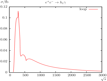
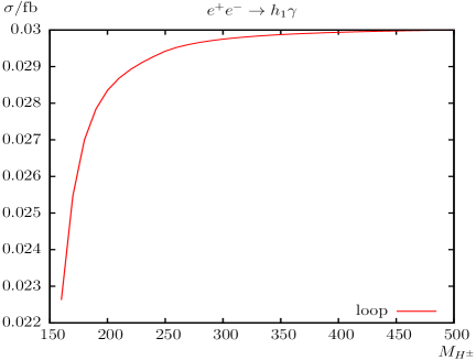
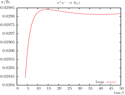
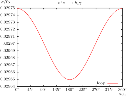
Figure 5: $\sigma(e^{+}e^{-}\to h_{1}\gamma)$. Loop induced (i.e. leading two-loop corrected) cross sections are shown with parameters chosen according to $\mathcal{S}$ (see Tab. 1), but with $\sqrt{s}=500\,\,\mathrm{GeV}$. the upper plots show the cross sections with $\sqrt{s}$ (left) and $M_{H^{\pm}}$ (right) varied; the lower plots show $t_{\beta}$ (left) and $\varphi_{A_{t}}$ (right) varied.

The largest contributions to $e^{+}e^{-}\to h_{1}\gamma$ are expected from loops involving top quarks and SM gauge bosons. The cross section is rather small for the parameter set chosen; see Tab. 1. As a function of $\sqrt{s}$ (upper left plot) a maximum of $\sim 0.1$ fb is reached around $\sqrt{s}\sim 250\,\,\mathrm{GeV}$, where several thresholds and dip effects overlap. the first peak is found at $\sqrt{s}\approx 283\,\,\mathrm{GeV}$, due to the threshold $m_{\tilde{\chi}_{1}^{\pm}}+m_{\tilde{\chi}_{1}^{\pm}}=\sqrt{s}$. A dip can be found at $m_{t}+m_{t}=\sqrt{s}\approx 346\,\,\mathrm{GeV}$. The next dip at $\sqrt{s}\approx 540\,\,\mathrm{GeV}$ is the threshold $m_{\tilde{\chi}_{2}^{\pm}}+m_{\tilde{\chi}_{2}^{\pm}}=\sqrt{s}$. The loop corrections for $\sqrt{s}$ vary between $0.1$ fb at $\sqrt{s}\approx 250\,\,\mathrm{GeV}$, $0.03$ fb at $\sqrt{s}\approx 500\,\,\mathrm{GeV}$ and $0.003$ fb at $\sqrt{s}\approx 3000\,\,\mathrm{GeV}$. Consequently, this process could be observable for larger ranges of $\sqrt{s}$. In particular in the initial phase with $\sqrt{s}=500\,\,\mathrm{GeV}$ [36] 30 events could be produced with an integrated luminosity of ${\cal L}=1\,\mbox{ab}^{-1}$. As a function of $M_{H^{\pm}}$ (upper right plot) we find an increase in $\mathcal{S}$ (but with $\sqrt{s}=500\,\,\mathrm{GeV}$), increasing the production cross sections from $0.023$ fb at $M_{H^{\pm}}\approx 160\,\,\mathrm{GeV}$ to about $0.03$ fb in the decoupling regime. This dependence shows the relevance of the SM gauge boson loops in the production cross section, indicating that the top quark loops dominate this production cross section. The variation with $t_{\beta}$ and $\varphi_{A_{t}}$ (lower row) is rather small, and values of $0.03$ fb are found in $\mathcal{S}$.

3 Conclusions

We reviewed the calculation of neutral MSSM Higgs boson production modes at $e^{+}e^{-}$ colliders with a two-particle final state, i.e. $e^{+}e^{-}\to h_{i}h_{j},h_{i}Z,h_{i}\gamma$ ($i,j=1,2,3$), allowing for complex parameters as presented in Ref. [32]. In the case of a discovery of additional Higgs bosons a subsequent precision measurement of their properties will be crucial to determine their nature and the underlying (SUSY) parameters. In order to yield a sufficient accuracy, one-loop corrections to the various Higgs boson production modes have to be considered. This is particularly the case for the high anticipated accuracy of the Higgs boson property determination at $e^{+}e^{-}$ colliders [15].

The evaluation of the processes (1) – (3) is based on a full one-loop calculation, also including hard and soft QED radiation. the renormalization is chosen to be identical as for the various Higgs boson decay calculations; see, e.g., Refs. [18, 19].

In our numerical scenarios we compared the tree-level production cross sections with the full one-loop corrected cross sections. In certain cases the tree-level cross sections are identical zero (due to the symmetries of the model), and in those cases we have evaluated the one-loop squared amplitude, $\sigma_{\text{loop}}\propto|{\cal M}_{\text{1-loop}}|^{2}$.

We found sizable corrections of $\sim 10-20\%$ in the $h_{i}h_{j}$ production cross sections. Substantially larger corrections are found in cases where the tree-level result is (accidentally) small and thus the production mode likely is not observable. The purely loop-induced processes of $e^{+}e^{-}\to h_{i}h_{i}$ could be observable, in particular in the case of $h_{1}h_{1}$ production. For the $h_{i}Z$ modes corrections around $10-20\%$, but going up to $\sim 50\%$, are found. the purely loop-induced processes of $h_{i}\gamma$ production appear observable for $h_{1}\gamma$ (but very challenging for $h_{2,3}\gamma$).

Only in very few cases a relevant dependence on $\varphi_{A_{t}}$ was found. Examples are $e^{+}e^{-}\to h_{1}h_{2}$ and $e^{+}e^{-}\to h_{3}Z$ (not shown), where a variation, after the inclusion of the loop corrections, of up to $10\%$ with $\varphi_{A_{t}}$ was found. In those cases neglecting the phase dependence could lead to a wrong impression of the relative size of the various cross sections.

Acknowledgements

The work of S.H. is supported in part by CICYT (grant FPA 2013-40715-P) and by the Spanish MICINN’s Consolider-Ingenio 2010 Program under grant MultiDark CSD2009-00064.

References

-
[1]
H. Nilles,
Phys. Rept. 110 (1984) 1;
R. Barbieri, Riv. Nuovo Cim. 11 (1988) 1. - [2] H. Haber, G. Kane, Phys. Rept. 117 (1985) 75.
- [3] J. Gunion, H. Haber, Nucl. Phys. B 272 (1986) 1.
-
[4]
A. Pilaftsis,
Phys. Rev. D 58 (1998) 096010
[arXiv:hep-ph/9803297];
A. Pilaftsis, Phys. Lett. B 435 (1998) 88 [arXiv:hep-ph/9805373]. - [5] D. Demir, Phys. Rev. D 60 (1999) 055006 [arXiv:hep-ph/9901389].
- [6] A. Pilaftsis and C. Wagner, Nucl. Phys. B 553 (1999) 3 [arXiv:hep-ph/9902371].
- [7] S. Heinemeyer, Eur. Phys. J. C 22 (2001) 521 [arXiv:hep-ph/0108059].
- [8] S. Heinemeyer, O. Stål and G. Weiglein, Phys. Lett. B 710 (2012) 201 [arXiv:1112.3026 [hep-ph]].
- [9] G. Aad et al. [ATLAS Collaboration], Phys. Lett. B 716 (2012) 1 [arXiv:1207.7214 [hep-ex]].
- [10] S. Chatrchyan et al. [CMS Collaboration], Phys. Lett. B 716 (2012) 30 [arXiv:1207.7235 [hep-ex]].
- [11] G. Aad et al. [ATLAS and CMS Collaborations], Phys. Rev. Lett. 114 (2015) 191803 [arXiv:1503.07589 [hep-ex]].
- [12] H. Baer et al., The International Linear Collider Technical Design Report - Volume 2: Physics, arXiv:1306.6352 [hep-ph].
-
[13]
TESLA Technical Design Report [TESLA Collaboration] Part 3,
Physics at an Linear Collider,
arXiv:hep-ph/0106315,
see: tesla.desy.de/new_pages/TDR_CD/start.html ;
K. Ackermann et al., DESY-PROC-2004-01. -
[14]
J. Brau et al. [ILC Collaboration],
ILC Reference Design Report Volume 1 - Executive Summary,
arXiv:0712.1950 [physics.acc-ph];
G. Aarons et al. [ILC Collaboration], International Linear Collider Reference Design Report Volume 2: Physics at the ILC, arXiv:0709.1893 [hep-ph]. - [15] G. Moortgat-Pick et al., Eur. Phys. J. C 75 (2015) 8, 371 [arXiv:1504.01726 [hep-ph]].
-
[16]
L. Linssen, A. Miyamoto, M. Stanitzki and H. Weerts,
arXiv:1202.5940 [physics.ins-det];
H. Abramowicz et al. [CLIC Detector and Physics Study Collaboration], Physics at the CLIC Linear Collider – Input to the Snowmass process 2013, arXiv:1307.5288 [hep-ex]. - [17] K. Williams, H. Rzehak, and G. Weiglein, Eur. Phys. J. C 71 (2011) 1669 [arXiv:1103.1335 [hep-ph]].
- [18] S. Heinemeyer and C. Schappacher, Eur. Phys. J C 75 (2015) 5, 198 [arXiv:1410.2787 [hep-ph]].
- [19] S. Heinemeyer and C. Schappacher, Eur. Phys. J C 75 (2015) 5, 230 [arXiv:1503.02996 [hep-ph]].
- [20] S. Heinemeyer, W. Hollik and G. Weiglein, Eur. Phys. J. C 16 (2000) 139 [arXiv:hep-ph/0003022].
-
[21]
R. Hempfling,
Phys. Rev. D 49 (1994) 6168;
L. Hall, R. Rattazzi and U. Sarid, Phys. Rev. D 50 (1994) 7048 [arXiv:hep-ph/9306309];
M. Carena, M. Olechowski, S. Pokorski and C. Wagner, Nucl. Phys. B 426 (1994) 269 [arXiv:hep-ph/9402253];
M. Carena, D. Garcia, U. Nierste and C. Wagner, Nucl. Phys. B 577 (2000) 577 [arXiv:hep-ph/9912516]. - [22] D. Noth and M. Spira, Phys. Rev. Lett. 101 (2008) 181801 [arXiv:0808.0087 [hep-ph]]; JHEP 1106 (2011) 084 [arXiv:1001.1935 [hep-ph]].
- [23] V. Barger, M. Berger, A. Stange and R. Phillips, Phys. Rev. D 45 (1992) 4128.
- [24] S. Heinemeyer and W. Hollik, Nucl. Phys. B 474 (1996) 32 [arXiv:hep-ph/9602318].
- [25] W. Hollik and J. Zhang, Phys. Rev. D 84 (2011) 055022 [arXiv:1109.4781 [hep-ph]].
-
[26]
A. Bredenstein, A. Denner, S. Dittmaier and M. Weber,
Phys. Rev. D 74 (2006) 013004
[arXiv:hep-ph/0604011];
JHEP 0702 (2007) 080
[arXiv:hep-ph/0611234];
A. Bredenstein, A. Denner, S. Dittmaier, A. Mück and M. Weber,
see: omnibus.uni-freiburg.de/~sd565/programs/prophecy4f/prophecy4f.html . - [27] M. Frank, T. Hahn, S. Heinemeyer, W. Hollik, H. Rzehak and G. Weiglein, JHEP 0702 (2007) 047 [arXiv:hep-ph/0611326].
-
[28]
S. Heinemeyer, W. Hollik and G. Weiglein,
Comput. Phys. Commun. 124 (2000) 76
[arXiv:hep-ph/9812320];
T. Hahn, S. Heinemeyer, W. Hollik, H. Rzehak and G. Weiglein, Comput. Phys. Commun. 180 (2009) 1426, see: www.feynhiggs.de . - [29] S. Heinemeyer, W. Hollik and G. Weiglein, Eur. Phys. J. C 9 (1999) 343 [arXiv:hep-ph/9812472].
- [30] G. Degrassi, S. Heinemeyer, W. Hollik, P. Slavich and G. Weiglein, Eur. Phys. J. C 28 (2003) 133 [arXiv:hep-ph/0212020].
- [31] T. Hahn, S. Heinemeyer, W. Hollik, H. Rzehak and G. Weiglein, Phys. Rev. Lett. 112 (2014) 141801 [arXiv:1312.4937 [hep-ph]].
- [32] S. Heinemeyer and C. Schappacher, arXiv:1511.06002 [hep-ph].
-
[33]
J. Frère, D. Jones and S. Raby,
Nucl. Phys. B 222 (1983) 11;
M. Claudson, L. Hall and I. Hinchliffe, Nucl. Phys. B 228 (1983) 501;
C. Kounnas, A. Lahanas, D. Nanopoulos and M. Quiros, Nucl. Phys. B 236 (1984) 438;
J. Gunion, H. Haber and M. Sher, Nucl. Phys. B 306 (1988) 1;
J. Casas, A. Lleyda and C. Muñoz, Nucl. Phys. B 471 (1996) 3 [arXiv:hep-ph/9507294];
P. Langacker and N. Polonsky, Phys. Rev. D 50 (1994) 2199 [arXiv:hep-ph/9403306];
A. Strumia, Nucl. Phys. B 482 (1996) 24 [arXiv:hep-ph/9604417]. -
[34]
A. Dobado, M. Herrero and S. Peñaranda,
Eur. Phys. J. C 17 (2000) 487
[arXiv:hep-ph/0002134];
J. Gunion and H. Haber, Phys. Rev. D 67 (1993) 075019 [arXiv:hep-ph/0207010];
H. Haber and Y. Nir, Phys. Lett. B 306 (1993) 327 [arXiv:hep-ph/9302228];
H. Haber, arXiv:hep-ph/9505240. - [35] The couplings can be found in HMix.ps.gz and MSSM.ps.gz as part of the FeynArts package [37].
- [36] T. Barklow, et al. arXiv:1506.07830 [hep-ex].
-
[37]
J. Küblbeck, M. Böhm and A. Denner,
Comput. Phys. Commun. 60 (1990) 165;
T. Hahn, Comput. Phys. Commun. 140 (2001) 418 [arXiv:hep-ph/0012260];
T. Hahn and C. Schappacher, Comput. Phys. Commun. 143 (2002) 54 [arXiv:hep-ph/0105349].
Program, user’s guide and model files are available via: www.feynarts.de .