Practical Riemannian Neural Networks

Abstract

We provide the first experimental results on non-synthetic datasets for the quasi-diagonal Riemannian gradient descents for neural networks introduced in [Oll15]. These include the MNIST, SVHN, and FACE datasets as well as a previously unpublished electroencephalogram dataset. The quasi-diagonal Riemannian algorithms consistently beat simple stochastic gradient gradient descents by a varying margin. The computational overhead with respect to simple backpropagation is around a factor $2$. Perhaps more interestingly, these methods also reach their final performance quickly, thus requiring fewer training epochs and a smaller total computation time.

We also present an implementation guide to these Riemannian gradient descents for neural networks, showing how the quasi-diagonal versions can be implemented with minimal effort on top of existing routines which compute gradients.

We present a practical and efficient implementation of invariant stochastic gradient descent algorithms for neural networks based on the quasi-diagonal Riemannian metrics introduced in [Oll15]. These can be implemented from the same data as RMSProp- or AdaGrad-based schemes [DHS11], namely, by collecting gradients and squared gradients for each data sample. Thus we will try to present them in a way that can easily be incorporated on top of existing software providing gradients for neural networks.

The main goal of these algorithms is to obtain invariance properties, such as, for a neural network, insensitivity of the training algorithm to whether a logistic or tanh activation function is used, or insensitivity to simple changes of variables in the parameters, such as scaling some parameters. Neither backpropagation nor AdaGrad-like schemes offer such properties.

Invariance properties are important as they reduce the number of arbitrary design choices, and guarantee that an observed good behavior in one instance will transfer to other cases when, e.g., different scalings are involved. In some cases this may alleviate the burden associated to hyper-parameter tuning: in turn, sensible hyper-parameter values sometimes become invariant.

Perhaps the most well-known invariant training procedure for statistical learning is the natural gradient promoted by Amari [Ama98]. However, the natural gradient is rarely used in practice for training neural networks. The main reason is that the Fisher information metric on which it relies is computationnally hard to compute. Different approximations have been proposed but can bring little benefits compared to the implementation effort; see for instance [RMB07, Mar14]. Moreover, it is not clear whether these approximations preserve the invariance properties. In the end, simpler techniques have been proposed to patch the flaws of the plain stochastic gradient descent. Using a balanced initialization with rectified linear units, dropout and SGD or AdaGrad can be enough to obtain very good results on many datasets. Nevertheless, these are tricks of the trade, little justified from a mathematical point of view.

The Riemannian framework for neural networks [Oll15] allows us to define several quasi-diagonal metrics, which exactly keep some (but not all) invariance properties of the natural gradient, at a smaller computational cost. The quasi-diagonal structure means that the gradient obtained at each step of the optimization is preconditioned by the inverse of a matrix which is almost diagonal, with a few well-chosen non-diagonal terms that make it easy to invert and have a special algebraic structure to ensure invariance with respect to some simple transformations such as changing from sigmoid to tanh activation function.

In this report, we assess the performance of these quasi-diagonal metrics (only tested on synthetic data in [Oll15]). They turn out to be quite competitive even after taking into account their computational overhead (a factor of about $2$ with respect to simple backpropagation). These methods consistently improve performance by various amounts depending on the dataset, and also work well with dropout. Especially, convergence is very fast early in the training procedure, which opens the door to using fewer epochs and shorter overall training times.

The code used in the experiments is available at
https://www.lri.fr/~marceau/code/riemaNNv1.zip

Invariance and gradient descents.

The simplest instance of parameter invariance is that of parameter scaling. Consider the classic gradient step

$$\theta\leftarrow\theta-\eta\,\nabla_{\!\theta}f\qquad\text{(vanilla gradient descent)}$$ (1)

where $\nabla_{\!\theta}f$ is the derivative of $f$ w.r.t. $\theta$. This iteration scheme has an homogeneity problem in terms of physical units: the unit of the derivative $\nabla_{\!\theta}f$ is the inverse of the unit of $\theta$. This means that the learning rate $\eta$ itself should have the homogeneity of $\theta^{2}$ for the gradient descent (1) to be homogeneous. This is one reason why sensible learning rates can change a lot from one problem to another.

AdaGrad-like methods [DHS11] solve one half of this problem by rescaling $\nabla_{\!\theta}f$ by its recent magnitude, so that it becomes of order $1$ (physically dimensionless). The learning rate $\eta$ then has the homogeneity of $\theta$, not $\theta^{2}$. This is particularly relevant when it is known in advance that relevant parameter values for $\theta$ are of order $1$ themselves; if not, the learning rate $\eta$ still needs to be set to a value compatible with the order of magnitude of $\theta$.

Another example of lack of invariance would be a change of input encoding. For example, if a network receives an image of a handwritten character in black and white or in white and black, or if the inputs are encoded with $0$ for black and $1$ for white or the other way round, this is equivalent to changing the inputs $x$ to $1-x$. A sigmoid unit with bias $b$ and weights $w_{i}$ reacts to $x$ the same way as a sigmoid unit reacts to $1-x$ if it has bias $b^{\prime}=b+\sum w_{i}$ and $w^{\prime}_{i}=-w_{i}$ (indeed, $b^{\prime}+\sum w^{\prime}_{i}(1-x_{i})=b+\sum w_{i}x_{i}$). However, the gradient descent on $(b^{\prime},w^{\prime})$ will behave differently from the gradient descent on $(b,w)$, because the correspondence mixes the weights with the bias. This leads to potentially different performances depending on whether the inputs are white-on-black or black-on-white, as shown on Figure 1. This specific problem is solved by using a tanh activation instead of a sigmoid, but it would be nice to have optimization procedures insensitive to such simple changes.

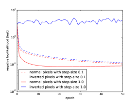
Figure 1: Classification task on MNIST with a non-convolutional 784-100-10 architecture. The figure shows the impact of inverting the pixels for two different step-sizes.

Mathematically, the problem is that the gradient descent (1) for a differentiable function $f\colon E\to{\mathbb{R}}$ defined on an abstract vector space $E$, is only well-defined after a choice of (orthonormal) basis. Indeed, at each point $\theta$ of $E$, the differential $\frac{\partial f}{\partial\theta}$ is a linear form (row vector) taking a vector $v$ as an argument and returning a scalar, $\frac{\partial f}{\partial\theta}\cdot v$, the derivative of $f$ in direction $v$ at the current point $\theta$. This differential is converted into a (row) vector by the definition of the gradient: $\nabla\!f$ is the unique vector such that $\frac{\partial f}{\partial\theta}\cdot v=\langle\nabla\!f,v\rangle$ for all vectors $v\in E$. This clearly depends on the definition of the inner product $\langle\cdot,\cdot\rangle$.

In an orthonormal basis, we simply have $\nabla\!f=(\frac{\partial f}{\partial\theta})^{\!\top}\!$. In a non-orthonormal basis, we have $\nabla\!f=M^{-1}(\frac{\partial f}{\partial\theta})^{\!\top}\!$ where $M$ is the symmetric, positive-definite matrix defining the inner product in this basis.

Using the vanilla gradient descent (1) amounts to deciding that whatever basis for $\theta$ we are currently working in, this basis is orthonormal. For two different parameterizations of the same intrinsic quantity, the vanilla gradient descent produces two completely different trajectories, and may eventually reach different local minima. As a striking example, if we consider all points obtained with one gradient step by varying the inner product, we span the whole half-space where $\frac{\partial f}{\partial\theta}\cdot v>0$.

Notice that an inner product defines a norm $\left\|v\right\|^{2}\mathrel{\mathop{:}}=\langle v,v\rangle$, which gives the notion of length between the points of $E$. The choice of the inner product makes it easier or more difficult for the gradient descent to move in certain directions. Indeed the gradient descent (1) is equivalent to

$$\theta\leftarrow\theta+\operatorname*{arg\,min}_{\delta\theta}\{f(\theta+\delta\theta)+\left\|\delta\theta\right\|^{2}/2\eta\}$$ (2)

up to $O(\eta^{2})$ for small learning rates $\eta$: this is a minimization over $f$, penalized by the norm of the update. Thus the choice of norm $\left\|\cdot\right\|$ clearly influences the direction of the update.

In general, it is not easy to define a relevant choice of inner product $\langle\cdot,\cdot\rangle$ if nothing is known about the problem. However, in statistical learning, it is possible to find a canonical choice of inner product that depends on the current point $\theta$. At each point $\theta$, the inner product between two vectors $v$, $v^{\prime}$ will be $\langle v,v^{\prime}\rangle_{\theta}=v^{\!\top}\!M(\theta)v^{\prime}$, where $M(\theta)$ is a particular positive definite matrix depending on $\theta$.

Several choices for $\langle v,v^{\prime}\rangle_{\theta}$ are given below, with the property that the scalar product $\langle v,v^{\prime}\rangle_{\theta}$, and the associated metric $\left\|v\right\|_{\theta}$, do not depend on a choice of basis for the vector space $E$. (Note that the matrix $M(\theta)$ does depend on the basis, since the expression of $v$ and $v^{\prime}$ as vectors does.) The resulting Riemannian gradient trajectory

$$\theta\leftarrow\theta-\eta\,M(\theta)^{-1}\frac{\partial f}{\partial\theta}^{\!\top}\!\qquad\text{(Riemannian gradient descent)}$$ (3)

is thus invariant to a change of basis in $E$. Actually, when the learning rate $\eta$ tends to $0$, the resulting continuous-time trajectory is invariant to any smooth homeomorphism of the space $E$, not only linear ones: this trajectory is defined on $E$ seen as a “manifold”.

Thus, the main idea behind invariance to coordinate changes is to define an inner product that does not depend on the numerical values used to represent the parameter $\theta$. We now give several such constructions together with the associated gradient update involving $M(\theta)^{-1}$.

Invariant gradient descents for neural networks.

In machine learning, we have a training dataset $\mathcal{D}=(x_{n},t_{n})_{n=1}^{N}$ where $x_{n}$ is a datum and $t_{n}$ is the associated target or label; we will denote $\mathcal{D}_{x}$ the set of all $x_{n}$’s in $\mathcal{D}$, and likewise for $\mathcal{D}_{t}$. Suppose that we have a model, such as a neural network, that for each input $x$ produces an output $y=y(x,\theta)$ depending on some parameter $\theta$ to be trained.

We suppose that the outputs $y$ are interpreted as a probability distribution over the possible targets $t$. For instance, in a classification task $y$ will be a vector containing the probabilities of the various possible labels. In a regression task, we might assume that the actual target follows a normal distribution centered at the predicted value $y$, namely $t_{n}=y(x_{n},\theta)+\sigma\mathcal{N}(0,\operatorname{Id})$ (in that case, $\sigma$ may be considered an additional parameter).

Let $p(t|y)$ be the probability distribution on the targets $t$ defined by the output $y$ of the network. We consider the log-loss function for input $x$ and target $t$:

$$\ell(t,x)\mathrel{\mathop{:}}=-\ln p(t|y(x,\theta))$$ (4)

For instance, with a Gaussian model $t=y(x,\theta)+\sigma\mathcal{N}(0,\operatorname{Id})$, this log-loss function is $\frac{(y-t)^{2}}{2\sigma^{2}}+\frac{\dim(y)}{2}\ln(2\pi\sigma^{2})$, namely, the square error $(y-t)^{2}$ up to a constant.

In this situation, there is a well-known choice of invariant scalar product on parameter space $\theta$, for which the matrix $M(\theta)$ is the Fisher information matrix on $\theta$,

$$M^{nat}(\theta)\mathrel{\mathop{:}}=\hat{\mathbb{E}}_{x\in\mathcal{D}_{x}}\mathbb{E}_{\tilde{t}\sim p(\cdot|y)}\left[\partial_{\theta}\ell(\tilde{t},x)(\partial_{\theta}\ell(\tilde{t},x))^{\!\top}\!\right]$$ (5)

where $\hat{\mathbb{E}}_{x\in\mathcal{D}_{x}}$ is the empirical average over the feature vectors of the dataset, and where $\partial_{\theta}\ell(\tilde{t},x)$ denotes the (column) vector of the derivatives of the loss with respect to the parameter $\theta$. For neural networks the latter is computed by backpropagation. Note that this expression involves the losses on all possible values of the targets $\tilde{t}$, not only the actual target for each data sample.

The natural gradient is the corresponding gradient descent (3), with $f\mathrel{\mathop{:}}=\mathbb{E}_{(x,t)\in\mathcal{D}}\ell(t,x)$ the average loss over the dataset:

$$\theta\leftarrow\theta-\eta\,M^{nat}(\theta)^{-1}\,\partial_{\theta}f$$ (6)

However, the natural gradient has several features that make it unsuitable for most large-scale learning tasks. Most of the literature on natural gradients for neural networks since Amari’s work [Ama98] deals with these issues.

First, the Fisher matrix is a full matrix of size $\dim(\theta)\times\dim(\theta)$, which makes it costly to invert if not impossible to store. Instead we will use a low-storage, easily inverted quasi-diagonal version of these matrices, which keeps many invariance properties of the full matrix.

Second, the Fisher matrix involves an expectation over “pseudo-targets” $\tilde{t}\sim p(\cdot|y)$ drawn from the distribution defined by the output of the network. This might not be a problem for classification tasks for which the number of possibilities for $t$ is small, but requires another approach for a Gaussian model if we want to avoid numerical integration over $\tilde{t}\sim y+\sigma\mathcal{N}(0,\operatorname{Id})$. We describe three ways around this: the outer product approximation, a Monte Carlo approximation, or an exact version which requires $\dim(y)$ backpropagations per sample.

Third, the Fisher matrix for a given value of the parameter $\theta$ is a sum over $x$ in the whole dataset. Thus, each natural gradient update would need a whole sweep over the dataset to compute the Fisher matrix for the current parameter. We will use a moving average over $x$ instead.

Let us discuss each of these points in turn.

Quasi-diagonal Riemannian metrics.

Instead of the full Fisher matrix, we use the quasi-diagonal reduction of $M^{-1}$, which involves computing and storing only the diagonal terms and a few off-diagonal terms of the matrix $M$. The quasi-diagonal reduction was introduced in [Oll15] to exactly keep some of the invariance properties of the Fisher matrix, at a price close to that of diagonal matrices.

Quasi-diagonal reduction uses a decomposition of the parameter $\theta$ into blocks. For neural networks, these blocks will be the parameters (bias and weights) incoming to each neuron, with the bias being the first parameter in each block. In each block, only the diagonal and the first row of the block are stored. Thus the number of non-zero entries to be stored is $2\dim(\theta)$ (actually slightly less, since in each block the first entry lies both on the diagonal and on the first row; in what follows, we include it in the diagonal and always ignore the first entry of the row).

Maintaining the first row in each block accounts for possible correlations between biases and weights, such as those appearing when the input values are transformed from $x$ to $1-x$ (see p. Invariance and gradient descents.). This is why the bias plays a special role here and has to be the first parameter in each block.

Quasi-diagonal metrics guarantee exact invariance to affine changes in the activations of each unit [Oll15, Section 2.3], including each input unit.

The operations we will need to perform on the matrix $M$ are of two types: computing $M$ by adding rank-one contributions of the form $vv^{\!\top}\!$ with $v=\partial_{\theta}\ell(\tilde{t},x)$ in (5), and applying the inverse of $M$ to a vector $v$ in the parameter update (3). For quasi-diagonal matrices these operations are explicited in Algorithms 2 and 1. The cost is about twice that of using diagonal matrices.

A by-product of this block-wise quasi-diagonal structure is that each layer can be considered independently. This enables to implement the computation of the metric in a modular fashion.

Function QDSolve($M$,$v$)

Data: Vector $v$; block decomposition for the components of $v$; matrix $M$ of size $\dim(v)\times\dim(v)$ of which only the diagonal and the first row in each block are known; regularization threshold $\varepsilon\geqslant 0$.

Result: Quasi-diagonal inverse $\mathrm{QD}(M)^{-1}.v$

foreach block of components of $v$ do

       $w\leftarrow$ $k$-th block of $v$;

       $\Delta\leftarrow$ diagonal of the $k$-th block of $M$;

       $r\leftarrow$ first row of the $k$-th block of $M$;

       $\Delta\leftarrow\Delta+\varepsilon$;

       Index the components of the block from $0$ to $n_{k}-1$;

       for i = 1 to $n_{k}-1$ (but NOT $i=0$) do

             $w_{i}\leftarrow\frac{\Delta_{0}w_{i}-r_{i}w_{0}}{\max\left(\Delta_{i}\Delta_{0}-r_{i}^{2},\,\varepsilon\right)}$;

            

       end for

      $w_{0}\leftarrow\frac{1}{\Delta_{0}}(w_{0}-\sum_{i=1}^{n_{k}-1}r_{i}w_{i})$;

       Store $w$ into the $k$-th block of the result;

      

end foreach

Algorithm 1 Pseudo-code for quasi-diagonal inversion. The case when the first rows are ignored ($q=0$) corresponds to a diagonal inversion $\mathrm{diag}(M+\varepsilon)^{-1}.v$. In our experiments, $\varepsilon$ is set to $10^{-8}$.

Function QDRankOneUpdate($M$,$v$,$\alpha$)

Data: Vector $v$; block decomposition for the components of $v$; matrix $M$ of size $\dim(v)\times\dim(v)$ of which only the diagonal and the first row in each block are known; real number $\alpha$.

Result: Rank-one update $M\leftarrow M+\alpha.\mathrm{QD}(vv^{\!\top}\!)$

foreach block of components of $v$ do

       $w\leftarrow$ $k$-th block of $v$;

       $\Delta\leftarrow$ diagonal of the $k$-th block of $M$;

       $r\leftarrow$ first row of the $k$-th block of $M$;

       $\Delta\leftarrow\Delta+\alpha\,w^{\odot 2}$;

       $r\leftarrow r+\alpha\,w_{0}\,w^{\!\top}\!$ with $w_{0}$ the first entry of $w$;

       Diagonal of the $k$-th block of $M$ $\leftarrow\Delta$;

       First row of the $k$-th block of $M$ $\leftarrow r$;

      

end foreach

Algorithm 2 Pseudo-code for quasi-diagonal accumulation: rank-one update of a quasi-diagonal matrix.

Online Riemannian gradient descent, and metric initialization.

As the Fisher matrix for a given value of the parameter $\theta$ is a sum over $x$ in the whole dataset, each natural gradient update would need a whole sweep over the dataset to compute the Fisher matrix for the current parameter. This is suitable for batch learning, but not for online stochastic gradient descent.

This can be alleviated by updating the metric via a moving average

$$M\leftarrow(1-\gamma)M+\gamma M_{\text{minibatch}}$$ (7)

where $\gamma$ is the metric update rate and where $M_{\text{minibatch}}$ is the metric computed on a small subset of the data, i.e., by replacing the empirical average $\hat{\mathbb{E}}_{x\in\mathcal{D}_{x}}$ with an empirical average $\hat{\mathbb{E}}_{x\in\mathcal{D}^{\prime}_{x}}$ over a minibatch $\mathcal{D}^{\prime}\subset\mathcal{D}$. Typically $\mathcal{D}^{\prime}$ is the same subset on which the gradient of the loss is computed in a stochastic gradient scheme. (This subset may be reduced to one sample.) This results in an online Riemannian gradient descent.

In practice, choosing $\gamma\approx\frac{1}{\#\text{minibatches}}$ ensures that the metric is mostly renewed after one whole sweep over the dataset. Usually we initialize the metric on the first minibatch ($\gamma=1$ for the first iteration), which is empirically better than using the identity metric for the first update. At startup when using very small minibatches (e.g., minibatches of size $1$) it may be advisable to initialize the metric on a larger number of samples before the first parameter update. (An alternative is to initialize the metric to $\operatorname{Id}$, but this breaks invariance at startup.)

Natural gradient, outer product, and Monte Carlo natural gradient.

The Fisher matrix involves an expectation over “pseudo-targets” $\tilde{t}\sim p(\cdot|y)$ drawn from the distribution defined by the output of the network: a backpropagation is needed for each possible value of $\tilde{t}$ in order to compute $\partial_{\theta}\ell(\tilde{t},x)$. This is acceptable only for classification tasks for which the number of possibilities for $t$ is small. Let us now describe three ways around this issue.

A first way to avoid the expectation over pseudo-targets $\tilde{t}\sim p(\cdot|y)$ is to only use the actual targets in the dataset. This defines the outer product approximation of the Fisher matrix

$$M^{OP}(\theta)\mathrel{\mathop{:}}=\hat{\mathbb{E}}_{(x,t)\in\mathcal{D}}\left[\partial_{\theta}\ell(\tilde{t},x)(\partial_{\theta}\ell(\tilde{t},x))^{\!\top}\!\right]$$ (8)

thus replacing $\hat{\mathbb{E}}_{x\in\mathcal{D}_{x}}\mathbb{E}_{\tilde{t}\sim p(\cdot|y)}$ with the empirical average $\hat{\mathbb{E}}_{(x,t)\in\mathcal{D}}$. For each training sample, we have to compute a rank-one matrix given by the outer product of the gradient for this sample, hence the name. This method has sometimes been used directly under the name “natural gradient”, although it has different properties, see discussion in [PB13] and [Oll15].

An advantage is that it can be computed directly from the gradient provided by usual backpropagation on each sample. The corresponding pseudocode is given in Algorithm 3 for a minibatch of size $1$.

Data: Dataset $\mathcal{D}$, a neural network structure with parameters $\theta$

Result: optimized parameters $\theta$

while not finish do

       retrieve a data sample $x$ and corresponding target $t$ from $\mathcal{D}$;

       forward $x$ through the network;

       compute loss $\ell(t,x)$;

       backpropagate and compute derivative of loss: $v\leftarrow\partial_{\theta}\ell(t,x)$;

       update quasi-diagonal metric using $vv^{\!\top}\!$:

       $M\leftarrow(1-\gamma)M$;

       QDRankOneUpdate($M$,$v$,$\gamma$);

       apply inverse metric: $v\leftarrow$ QDSolve($M$,$v$);

       update parameters: $\theta\leftarrow\theta-\eta v$;

      

end while

Algorithm 3 Online gradient descent using the quasi-diagonal outer product metric.

A second way to proceed is to replace the expectation over pseudo-targets $\tilde{t}$ with a Monte Carlo approximation using $n_{MC}$ samples:

$$M^{MCnat}(\theta)\mathrel{\mathop{:}}=\mathbb{E}_{x\in\mathcal{D}_{x}}\left[\frac{1}{n_{MC}}\sum_{i=1}^{n_{MC}}\partial_{\theta}\ell(\tilde{t}_{i},x)(\partial_{\theta}\ell(\tilde{t}_{i},x))^{\!\top}\!\right]$$ (9)

where each pseudo-target $\tilde{t}_{i}$ is drawn from the distribution $p(\tilde{t}|y)$ defined by the output of the network for each input $x$. This is the Monte Carlo natural gradient [Oll15]. We have found that $n_{MC}=1$ (one pseudo-target for each input $x$) works well in practice.

The corresponding pseudocode is given in Algorithm 4 for a minibatch of size $1$ and $n_{MC}=1$.

Data: Dataset $\mathcal{D}$, a neural network structure with parameters $\theta$

Result: optimized parameters $\theta$

while not finish do

       retrieve a data sample $x$ and corresponding target $t$ from $\mathcal{D}$;

       forward $x$ through the network;

       compute loss $\ell(t,x)$;

       backpropagate and compute derivative of loss: $v\leftarrow\partial_{\theta}\ell(t,x)$;

       generate pseudo-target $\tilde{t}$ according to probability distribution defined by the output layer $y$ of the network: $\tilde{t}\sim p(\cdot|y)$;

       backpropagate and compute derivative of loss for $\tilde{t}$: $\tilde{v}\leftarrow\partial_{\theta}\ell(\tilde{t},x)$;

       update quasi-diagonal metric using $\tilde{v}\tilde{v}^{\!\top}\!$:

       $M\leftarrow(1-\gamma)M$;

       QDRankOneUpdate($M$,$\tilde{v}$,$\gamma$);

       apply inverse metric: $v\leftarrow$ QDSolve($M$,$v$);

       update parameters: $\theta\leftarrow\theta-\eta v$;

      

end while

Algorithm 4 Online gradient descent using the quasi-diagonal Monte Carlo natural gradient, with $n_{MC}=1$.

The third option is to compute the expectation over $\tilde{t}$ exactly using algebraic properties of the Fisher matrix. This can be done at the cost of $\dim(y)$ backpropagations per sample instead of one. The details depend on the type of the output layer, as follows.

If the output is a softmax over $K$ categories, one can just write out the expectation explicitly:

$$M^{nat}(\theta)=\hat{\mathbb{E}}_{x\in\mathcal{D}_{x}}\left[\sum_{\tilde{t}=1}^{K}p(\tilde{t}|y)\,\partial_{\theta}\ell(\tilde{t},x)(\partial_{\theta}\ell(\tilde{t},x))^{\!\top}\!\right]$$ (10)

so that the metric is a sum of rank-one terms over all possible pseudo-targets $\tilde{t}$, weighted by their predicted probabilities.

If the output model is multivariate Gaussian with diagonal covariance matrix $\Sigma=\mathrm{diag}(\sigma_{k}^{2})$ ($\Sigma$ may be known or learned), i.e., $t=y+\mathcal{N}(0,\Sigma)$, then one can prove that the Fisher matrix is equal to

$$M^{nat}(\theta)=\hat{\mathbb{E}}_{x\in\mathcal{D}_{x}}\left[\sum_{k=1}^{K}\frac{1}{\sigma_{k}^{2}}\,\partial_{\theta}y_{k}(\partial_{\theta}y_{k})^{\!\top}\!\right]$$ (11)

where $y_{k}$ is the $k$-th component of the network output. The derivative $\partial_{\theta}y_{k}$ can be obtained by backpropagation if the backpropagation is initialized by setting the $k$-th output unit to $1$ and all other units to $0$. This has to be done separately for each output unit $k$. Thus, for each input $x$ the metric is a contribution of several rank-one terms $\partial_{\theta}y_{k}(\partial_{\theta}y_{k})^{\!\top}\!$ obtained by backpropagation, and weighted by $1/\sigma_{k}^{2}$.

Another model for predicting binary data is the Bernoulli output, in which the activities of output units $y_{k}\in[0;1]$ are interpreted as probabilities to have a $0$ or a $1$. This case is similar to the Gaussian case up to replacing $\frac{1}{\sigma_{k}^{2}}$ with $\frac{1}{y_{k}(1-y_{k})}$ (inverse variance of the Bernoulli variable defined by output unit $k$).

The pseudocode for the quasi-diagonal natural gradient is given in Algorithm 5.

Data: Dataset $\mathcal{D}$, a neural network structure with parameters $\theta$, a quasi-diagonal metric $M$

Result: optimized parameters $\theta$

while not finish do

       retrieve a data sample $x$ and corresponding target $t$ from $\mathcal{D}$;

       forward $x$ through the network;

       compute loss $\ell(t,x)$;

       backpropagate and compute derivative of loss: $v\leftarrow\partial_{\theta}\ell(t,x)$;

       $M\leftarrow(1-\gamma)M$;

       Depending on output layer interpretation:

       Categorical output with classes {1,…,K}:

       for each class $\tilde{t}$ from $1$ to $K$ do

             Set $\tilde{t}$ as the pseudo-target;

             $\alpha\leftarrow p(\tilde{t}|y)$ ;

             backpropagate and compute derivative of loss for $\tilde{t}$: $\tilde{v}\leftarrow\partial_{\theta}\ell(\tilde{t},x)$;

             update quasi-diagonal metric using $\tilde{v}\tilde{v}^{\!\top}\!$:

             QDRankOneUpdate($M$,$\tilde{v}$,$\gamma\alpha$);

            

       end for

      Gaussian output (square loss) with variance $\mathrm{diag}(\sigma_{k}^{2})$, $k=1,\ldots,K$:

       for each output unit $k$ from $1$ to $K$ do

             $\alpha\leftarrow 1/\sigma_{k}^{2}$ ;

             $\tilde{v}\leftarrow\partial_{\theta}y^{k}$ (obtained by setting backpropagated values on the $k$-th output unit to $1$, all the others to $0$, and backpropagating);

             update quasi-diagonal metric using $\tilde{v}\tilde{v}^{\!\top}\!$:

             QDRankOneUpdate($M$,$\tilde{v}$,$\gamma\alpha$);

            

       end for

      apply inverse metric: $v\leftarrow$ QDSolve($M$,$v$);

       update parameters: $\theta\leftarrow\theta-\eta v$;

      

end while

Algorithm 5 Online gradient descent using the quasi-diagonal natural gradient.

Notably, the OP and Monte Carlo approximation both keep the invariance properties of the natural gradient. This is not the case for other natural gradient approximations such as the blockwise rank-one approximation used in [RMB07].

Each of these approaches has its strengths and weaknesses. The (quasi-diagonal) OP is easy to implement as it relies only on quantities (the gradient for each sample) that have been computed anyway, while the Monte Carlo and exact natural gradient must make backpropagation passes for other values of the output of the network.

When the model fits the data well, the distribution $p(\tilde{t}|y)$ gives high probability to the actual targets $t$ and thus, the OP metric is a good approximation of the Fisher metric. However, at startup, the model does not fit the data and OP might poorly approximate the Fisher metric. Similarly, if the output model is misspecified, OP can perform badly even in the last stages of optimization; for instance, OP fails miserably to optimize a quadratic function in the absence of noise, an example to keep in mind.

The exact quasi-diagonal natural gradient is only affordable when the dimension of the output $y$ of the network is not too large, as $\dim(y)$ backpropagations per sample are required. Thus the OP and Monte Carlo approximations are appealing when output dimensionality is large, as is typical for auto-encoders. However, in this case the probability distribution $p(\tilde{t}|y)$ is defined over a high-dimensional space, and the OP approximation using the single deterministic point $\tilde{t}=t$ may be poor. (In preliminary experiments from [Oll15], the OP approximation performed poorly for an auto-encoding task.) On the other hand, Monte Carlo integration often performs relatively well in high dimension, and might be a sensible choice for large-dimensional outputs such as in auto-encoders.

Still, the choice between these three options is largely experimental. Since all three have closely related implementations (Algorithms 3–5), they can be compared with little effort.

Diagonal versions: From AdaGrad to OP, and invariance properties.

The algorithms presented above with quasi-diagonal matrices also have a diagonal version, obtained by simply discarding the non-diagonal terms. (This breaks affine invariance.)

For instance, the update for diagonal OP (DOP) reads

$$M^{DOP}\leftarrow(1-\gamma)M^{DOP}+\gamma\,\mathrm{diag}(\partial_{\theta}\ell\,\partial_{\theta}\ell^{\!\top}\!)$$ (12)

where $\partial_{\theta}\ell$ is the derivative of the loss $\ell$ for the current sample. This can be rewritten on the vector of diagonal entries of $M^{DOP}$ as

$$\mathrm{diag}(M^{DOP})\leftarrow(1-\gamma)\mathrm{diag}(M^{DOP})+\gamma\,(\partial_{\theta}\ell)^{\odot 2}$$ (13)

This update is the same as the one used in the family of AdaGrad or RMSProp algorithms, except that the latter use the square root of $M$ in the final parameter update:

$$\theta\leftarrow\theta-\eta M_{Ada}^{-1/2}\partial_{\theta}\ell$$ (14)

where $M_{Ada}$ follows the same update as $M^{DOP}$. Thus, although AdaGrad shares a similar framework with DOP, it is not naturally interpreted as a Riemannian metric on parameter space (there is no well-defined trajectory on the parameter space seen as a manifold), because taking the element-wise square-root breaks all potential invariances.

To summarize, the diagonal versions DOP, DMCNat and DNat are exactly invariant to rescaling of each parameter component. In addition, the quasi-diagonal versions of these algorithms are exactly invariant to an affine change in the activity of each unit, including the activities of input units; this covers, for instance, using tanh instead of sigmoid, or using white-on-black instead of black-on-white inputs. In contrast, to our knowledge AdaGrad has no invariance properties (the values of the gradients $M_{Ada}^{-1/2}\partial_{\theta}\ell$ are scale-invariant in AdaGrad, but not the resulting parameter trajectories, since the parameter $\theta$ is updated by the same value whatever its scale).

Experimental studies.

We demonstrate the invariance and efficiency of Riemannian gradient descents through experiments on a series of classification and regression tasks. For each task, we choose an architecture and an activation function, and we perform a grid search over various powers of $10$ for the step-size. The step-size is kept fixed during optimization. Then, for each algorithm, we report the curve associated with the best step size. The algorithms tested are standard stochastic gradient descent (SGD), AdaGrad, and the diagonal and quasi-diagonal versions of OP, of Monte Carlo natural gradient (with only one sample), and of the exact natural gradient when the dimension of the output layer is not too large to compute it.

First, we study the classification task on MNIST [LC] and the Street View Housing Numbers (SVHN)[NWC⁺11]. We work in a permutation-invariant setting, i.e., the network is not convolutional and the natural topology of the image is not taken into account in the network structure. We also converted the SVHN images into grayscale images in order to reduce the dimensionality of the input.

Note that these experiments are small-scale and not geared towards obtaining state-of-the-art performance, but aim at comparing the behavior of several algorithms on a common ground, with relatively small architectures.

Experiments on the classification task confirm that Riemannian algorithms are both more invariant and more efficient than non-invariant algorithms. In the first experiment we train a network with two hidden layers and 800 hidden units per layer, without any regularization, on MNIST; the results are given on Figure 2.

Quasi-diagonal algorithms (plain lines) converge faster than the other algorithms. Especially, they exhibit a steep slope for the first few epochs, and quickly reach a satisfying performance. Their trajectories are also very similar for every activation function. The trajectories of SGD, AdaGrad, and the diagonally approximated Riemannian algorithms are more variable: for instance, SGD is close enough to the quasi-diagonal algorithms with ReLU activation but not with sigmoid or tanh, and AdaGrad performs well with tanh but not with sigmoid or ReLU. Finally, the Monte Carlo QD natural gradient seems to be a very good approximation of the exact QD natural gradient, even with only one Monte Carlo sample. This may be related to simplicity of the problem, since the probabilities of the output layer converges rapidly to their optimal values.

Quasi-diagonal algorithms are also efficient in practice. Their computational cost is reasonably close to pure SGD, as shown on Table 1, with an overhead of about $2$ as could be expected. They are often much faster to learn in terms of number of training examples processed, compared to SGD or AdaGrad.

The quasi-diagonal algorithms also behave well with the dropout regularization [SHK⁺14], as can be seen on Figure 3. Several runs went below $1\%$ classification error with this simple 800-800, permutation-invariant architecture. Three groups of trajectories are clearly visible on Figure 3, with AdaGrad fairly close to the quasi-diagonal algorithms on this example. There is a clear difference between the quasi-diagonal algorithms and their diagonal approximations: keeping only the diagonal breaks the invariance to affine transormations of the activities, which thus appears as a key factor here as well as in almost all experiments below.

Algorithm	mean (std)
SGD	29.10 (0.76)
AdaGrad	33.39 (2.26)
RiemannDOP	42.44 (1.26)
RiemannQDOP	56.68 (3.75)
RiemannDMCNat	58.17 (4.57)
RiemannQDMCNat	68.01 (2.35)
RiemannDNat	120.16 (0.34)
RiemannQDNat	129.76 (0.34)

Table 1: Computational time per epoch for a 784-800-800-10 architecture on MNIST with minibatch of size 500 on a CPU.

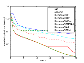
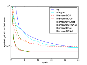
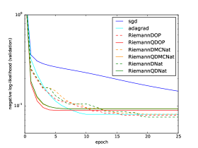
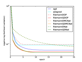
Figure 2: Classification task on MNIST with a non-convolutional 784-800-800-10 architecture without regularization. We use a sigmoid (upper left and upper right), a tanh (lower left) and a ReLU (lower right).

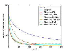
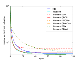
Figure 3: Classification task on MNIST with a non-convolutional 784-800-800-10 architecture and sigmoid (left) or ReLU (right). The network is regularized with dropout.

On a more difficult dataset, the permutation invariant SVHN with grayscale images, we observe the same pattern as for the MNIST dataset, with the quasi-diagonal algorithms leading on SGD and AdaGrad (Figure 4). However, ReLU is severely impacting the diagonal approximations of the Riemannian algorithms: they diverge for step-sizes larger than $10^{-5}$. This emphasizes once more the importance of the quasi-diagonal terms.

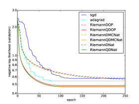
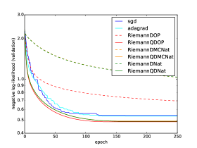
Figure 4: Classification task on SVHN with a non-convolutional 1024-800-800-10 architecture and sigmoid (left) or ReLU (right). The network is not regularized.

We also test the algorithm on a deeper architecture on the MNIST dataset, with the goal of testing whether Riemannian algorithms handle “vanishing gradients” [Hoc91] better. We use a sparse network with a connectivity factor of 10 incoming weights per unit. The connection graph is built from the output to the input by randomly choosing, for each unit, ten units from the previous layer. The last output layer is fully connected. We choose a network with 8 hidden layers with the following architecture: 2560-1280-640-320-160-80-40-20. The number of parameters is relatively small (56310 parameters), and since the architecture is deep, this should be a difficult problem already as a purely optimization task (i.e., already on the training set). From Figure 5, we observe three groups: SGD is very slow to converge, while the quasi-diagonal algorithms reach quite small loss values on the training set (around $10^{-4}$ or $10^{-5}$) and perform reasonably well on the validation set. AdaGrad and the diagonal approximations stand in between. Once more, quasi-diagonal algorithms have a steep descent during the first epochs. Note the various plateaus of several algorithms when they reach very small loss values; this may be related to numerical issues for such small values, especially as we used a fixed step size. Indeed, most of the plateaus are due to minor instabilities which cause small rises of the loss values. This may disappear with step sizes tending to $0$ on a schedule.

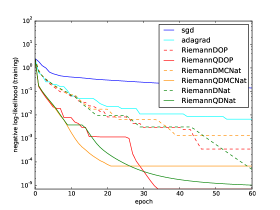
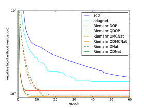
Figure 5: Classification task on MNIST with a 784-2560-1280-640-320-160-80-40-20-10 architecture and sigmoid activation function. We use a sparse network (sparsity=10) with 56310 parameters without regularization. The training trajectory is on the left and the validation trajectory is on the right.

Next, we evaluate the Riemannian gradient descents on a regression task, namely, reconstruction of the inputs. We use the MNIST dataset and the faces in the wild dataset (FACES) [HJLM07], again in a permutation-invariant non-convolutional setting. For the FACES dataset, we crop a border of 30 pixels around the image and we convert it into a grayscale image. The faces are still recognizable with this lower resolution variant of the dataset. For this dataset, we use an autoencoder with three hidden layers (256-64-256) and a Gaussian output.

We also use a dataset of EEG signal recordings. These are raw signals captured with 56 electrodes (56 features) with 12 000 measurements. The goal is to compress the signals with very few hidden units on the bottleneck layer, and still be able to reconstruct the signal well. Notice that these signals are very noisy. For this dataset we use an autoencoder with seven hidden layers (32-16-8-4-8-16-32) and a Gaussian output.

In such a setting, the outer product and Monte Carlo natural gradient are well-suited (Algorithms 3–4), but the exact natural gradient (Algorithm 5) scales like the dimension of the output and thus is not reasonable (except for the EEG dataset).

The first experiment, depicted on Figure 6, consists in minimizing the mean square error of the reconstruction for the FACES dataset. (The mean square error can be interpreted in terms of a negative log-likelihood loss by defining the outputs as the mean vector of a multivariate Gaussian with variance equals to one for every output.)

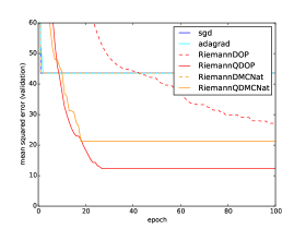
Figure 6: Reconstruction task on FACES (left) with a 2025-256-64-256-2025 architecture. The network is not regularized, has a sigmoid activation function and a Gaussian output with unit variances.

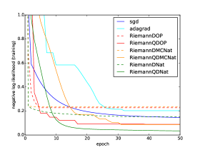
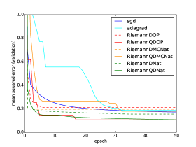
Figure 7: Reconstruction task on EEG with a 56-32-16-8-4-8-16-32-56 architecture. The network is not regularized, has a sigmoid activation function and a Gaussian output with unit variances.

For this experiment, SGD, AdaGrad and RiemannDMCNat are stuck after one epoch around a mean square error of 45. In fact, they continue to minimize the loss function but very slowly, such that it cannot be observed on the figure. This behavior is consistent for every step-size for these algorithms, and may be related to finding a bad local optimum. On the other hand, with a small step-size, the quasi-diagonal algorithms successfully decrease the loss well below 45, and do so in few epochs, yielding a sizeable gain in performance.

On the EEG dataset (Figure 7), the gain in performance of the quasi-diagonal algorithms is also notable, though not quite as spectacular as on FACES.

Finally we trained an autoencoder with a multivariate Gaussian output on MNIST, where the variances of the outputs are also learned at the same time as the network parameters. As depicted on Figure 8, the performances are consistent with the previous experiments. Interestingly, QDOP is the most efficient algorithm even though the real noise model over the outputs departs from the diagonal Gaussian model on the output, so that the OP approximation to the natural gradient is not necessarily accurate.

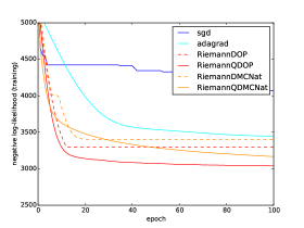
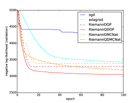
Figure 8: Reconstruction task on MNIST with a 784-256-64-256-784 architecture (autoencoder), a sigmoid activation function and a Gaussian ouput with learned variances.

Learning rates and regularization.

Riemannian algorithms are still sensitive to the choice of the gradient step-size (like classical methods), and also to the numerical regularization term (the $\varepsilon$ in procedure QDSolve), which was set to $\varepsilon=10^{-8}$ in all our experiments. The numerical regularization term is necessary to ensure that the metric is invertible. However, this term also breaks some invariance and thus, it should be chosen as small as possible, in the limit of numerical stability. In practice, RiemannQDMCNat seems to be more sensitive to numerical stability than RiemannQDOP and RiemannQDNat.

Moreover, both the Riemannian algorithms and AdaGrad use an additional hyperparameter $\gamma$, the decay rate used in the moving average of the matrix $M$ and of the square gradients of AdaGrad. The experiments above use $\gamma=0.01$.

Conclusions.

• The gradient descents based on quasi-diagonal Riemannian metrics, including the quasi-diagonal natural gradient, can easily be implemented on top on an existing framework which computes gradients, using the routines QDRankOneUpdate and QDSolve. The overhead with respect to simple SGD is a factor about $2$ in typical situations.

• The resulting quasi-diagonal learning algorithms perform quite consistently across the board whereas performance of simple SGD or AdaGrad is more sensitive to design choices such as using ReLU or sigmoid activations.

• The quasi-diagonal learning algorithms exhibit fast improvement in the first few epochs of training, thus reaching their final performance quite fast. The eventual gain over a well-tuned SGD or AdaGrad trained for many more epochs can be small or large depending on the task.

• The quasi-diagonal Riemannian metrics widely outperform their diagonal approximations (which break affine invariance properties). The latter do not necessarily perform better than classical algorithms. This supports the specific influence of invariance properties for performance, and the interest of designing algorithms with such invariance properties in mind.

References

- [Ama98] Shun-Ichi Amari. Natural gradient works efficiently in learning. Neural Comput., 10(2):251–276, February 1998.
- [DHS11] John C. Duchi, Elad Hazan, and Yoram Singer. Adaptive subgradient methods for online learning and stochastic optimization. Journal of Machine Learning Research, 12:2121–2159, 2011.
- [HJLM07] Gary B. Huang, Vidit Jain, and Erik Learned-Miller. Unsupervised joint alignment of complex images. In ICCV, 2007.
- [Hoc91] Sepp Hochreiter. Untersuchungen zu dynamischen neuronalen Netzen. Masters Thesis, Technische Universität München, München, 1991.
- [LC] Yann Lecun and Corinna Cortes. The MNIST database of handwritten digits.
- [Mar14] James Martens. New perspectives on the natural gradient method. CoRR, abs/1412.1193, 2014.
- [NWC+11] Yuval Netzer, Tao Wang, Adam Coates, Alessandro Bissacco, Bo Wu, and Andrew Y. Ng. Reading digits in natural images with unsupervised feature learning. In NIPS Workshop on Deep Learning and Unsupervised Feature Learning 2011, 2011.
- [Oll15] Yann Ollivier. Riemannian metrics for neural networks I: feedforward networks. Information and Inference, 4(2):108–153, 2015.
- [PB13] Razvan Pascanu and Yoshua Bengio. Natural gradient revisited. CoRR, abs/1301.3584, 2013.
- [RMB07] Nicolas Le Roux, Pierre-Antoine Manzagol, and Yoshua Bengio. Topmoumoute online natural gradient algorithm. In John C. Platt, Daphne Koller, Yoram Singer, and Sam T. Roweis, editors, Advances in Neural Information Processing Systems 20, Proceedings of the Twenty-First Annual Conference on Neural Information Processing Systems, Vancouver, British Columbia, Canada, December 3-6, 2007, pages 849–856. Curran Associates, Inc., 2007.
- [SHK+14] Nitish Srivastava, Geoffrey E. Hinton, Alex Krizhevsky, Ilya Sutskever, and Ruslan Salakhutdinov. Dropout: a simple way to prevent neural networks from overfitting. Journal of Machine Learning Research, 15(1):1929–1958, 2014.