Delocalization in One-Dimensional Tight-Binding Models with Fractal Disorder II: Existence of Mobility Edge

Abstract

In the previous work, we investigated the correlation-induced localization-delocalization transition (LDT) of the wavefunction at band center ($E=0$) in the one-dimensional tight-binding model with fractal disorder [Yamada, EPJB (2015) 88, 264]. In the present work, we study the energy ($E\neq 0$) dependence of the normalized localization length (NLL) and the delocalization of the wavefunction at the different energy in the same system. The mobility edges in the LDT arise when the fractal dimension of the potential landscape is larger than the critical value depending on the disorder strength, which is consistent with the previous result. In addition, we present the distribution of individual NLL and Lyapunov exponent in the system with LDT.

1 Introduction

All eigenstates are exponentially localized in one-dimensional disordered systems (1DDS) with uncorrelated on-site disorder ishii73 ; abrahams79 ; lifshiz88 . Recently, the study of delocalization phenomena in the 1DDS with long-range correlation have been performed using analytical as well as numerical methods yamada91 ; oliveira01 ; pinto04 ; esmailpour07 ; sales12 ; cheraghchi05 ; lazoa10 ; moura98 ; izrailev99 ; izrailev12 . In particular, many authors could numerically observe the correlation-induced localization-delocalization transition (LDT) in the 1D tight-binding model (TBM) by using the same potential sequences with power spectrum $S(f)\sim 1/f^{\alpha}$($\alpha\geq 2$) using Fourier filtering method (FFM), where $f$ denotes frequency moura98 ; izrailev99 ; zhang02 ; shima04 ; kaya07 ; kaya09 ; gong10 ; croy11 ; deng12 ; gong12 ; albrecht12 .

Very recently, Garcia and Cuevas modeled the sequences with the power-law spectrum by Weierstrass function with fractal dimension $D$ and studied the transition based on the differentiability of the disorder potential as a necessary condition for the delocalization garcia09 ; garcia10 ; petersen12 ; petersen13 . As a result, they could numerically demonstrate that the LDT takes place at the critical value $D_{c}=3/2$ by means of the distribution of the energy level-spacing in the weak disorder limit.

In the previous paper yamada15 , we have numerically reported that the finite-size scaling analysis for the normalized localization length (NLL) at the band center ($E=0$) suggests the existence of the LDT around $D_{c}\simeq 3/2$ independent of the potential strength in the relatively weak disorder regime, as suggested by Garcia and Cuevas. On the other hand, in the relatively strong disorder regime, the critical fractal dimension $D_{c}$ arrives at a smaller value than $3/2$ when varying the potential strength yamada15 . In addition, the existence of the power-law localized states has been observed in the case of relatively weak disorder strength for $D\geq 3/2$, which implies zero Lyapunov exponent. Such a power-law localization have been also observed in off-diagonal disordered systems and quantum percolation systems xiong01 ; igor08 ; bellando14 .

What remains a question is the delocalization of the other energy states of the TBM with the Weierstrass potential. In this study, therefore, we numerically investigate the delocalized behavior of the other energy states ($E\neq 0$) using the system size dependence of the NLL. We demonstrate the presence of the mobility edges and the power-law localized behavior for $D\gtrsim 3/2$ in the weak disorder cases. The critical value of $D$ decreases with increasing the disorder strength $W$ in the strong disorder regime.

On the other hand, the statistical properties of the individual NLL and Lyapunov exponent have not beend studied in detail for the 1DDS with LDT, although the anomalous fluctuation might be expexcted yamada91 ; pinto04 . With this in mind, we investigate here the statistical properties over ensamble and are able to verify the presence of the anomalous fluctuation, as well as to reveal the details of the systemsize dependence by taking large system size and large ensamble size as much as possible.

This paper is organized as follows. In the next section, we briefly introduce the 1DDS with the Weierstrass potential and some eigenstates. In Sect.3, we present global behavior of the $E-$dependence and $N-$dependence in the LDT by the numerical calculation of the NLL. In Sect.4, we present statistical distribution and convergence property of the individual NLL and Lyapunov exponent with increasing the system size for the band edge state. Summary and discussion are presented in the last section.

2 Model

We consider the one-dimensional tight-binding Hamiltonian describing single-particle electronic states as

$$H=\sum_{n=1}^{N}V(n)C_{n}^{\dagger}C_{n}+\sum_{n=1}^{N-1}C_{n}^{\dagger}C_{n+1}+H.C.,$$ (1)

where $C_{n}^{\dagger}$($C_{n}$) is the creation (annihilation) operator for the one-electron state at site $n$. The $\{V(n)\}_{n=0}^{N}$ and $W$ are the disordered on-site energy sequence and the strength, respectively. The amplitude of the quantum state $|\Phi>$ is given by $\phi(n)\equiv<\Phi|C_{n}^{\dagger}C_{n}|\Phi>$ in the site representation. To model the correlated disorder potential for $V(n)$($n\leq N$) in Eq.(1), we use the following form:

$$V(n)=C\sum_{k=0}^{L}\frac{\sin(2\pi a^{k}n/N+\varphi_{k})}{a^{(2-D)k}},$$ (2)

where $a$ is a constant value ($a>1$) related the scale-invariance and $D$ is a fractal dimension ($1<D<2$). $\{\varphi_{k}\}_{k=0}^{L}$ are random independent variables chosen in the interval $[0,2\pi]$. $C$ is the normalization constant which is determined by a condition

$$\sqrt{<V(n)^{2}>-<V(n)>^{2}}=1,$$ (3)

where $\langle...\rangle$ indicates the average over realization of the phases in Eq.(2). If we set $n/N=x$, $\varphi_{k}=0$, the potential sequence becomes the ”Weierstrass function” being continuous and indifferentiable everywhere by taking a continuous limit $N\to\infty$ and $L\to\infty$. Therefore, the potential will be shortly transfered to as ”Weierstrass potential” in this paper, and we set $a=2$ and $L=50$ through this report without loss of the generality and accuracy of the numerical calculation. Figure 1 shows some potential landscapes. We can see that the landscape becomes smooth as the fractal dimension $D$ decreasing. Note that the condition $\alpha\geq 2$ for the LDT corresponds to a condition $D\leq 3/2$ because the power spectrum $S(f)$ of the Weierstrass function is empirically characterized by $S(f)\sim\frac{1}{f^{5-2D}}$. The smoothness of the potential fluctuation can also induce the delocalization of the quantum states, which property is directly related to analyticity of the potential function in the continuum limit.

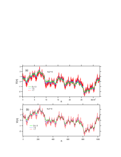
Figure 1: (Color online) Typical on-site energy landscape $V(n)$ generated by the Eq.(2) and the normalization (3) with $D=1.3,1.5,1.7$. (a)$N=2^{15}$, (b)$N=2^{10}$.

Garcia and Cuevas garcia09 ; garcia10 have numerically found that LDT at $D_{c}=3/2$ for the sufficiently weak disorder regime by using the nearest-neighbor level-space distribution of the energy spectrum. It is useful to look at typical eigenstates directly to ratinalize the effects of the fluctuation of the potential on the delocalization. Some typical eigenstates are shown in Fig.2. The state close to the band center as well as the one around band edge are localized for $D=1.7$, while the state near band center is delocalized for $D=1.3$. These features are consistent with our previous work yamada15 . For small values of $L$ some typical potential landscapes and the eigenstates are given in appendix A. In the next section, we investigate the energy dependence of the quantum states.

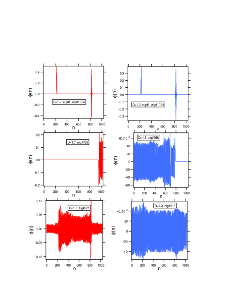
Figure 2: (Color online) Comparison of some eigenstates $\{\phi(n)\}$ for the Weierstrasse potential in Fig.1(b) with $D=1.7$ (left panels), $D=1.3$ (right panels). $W=0.75$, $N=2^{10}$ and rigid boundary condition are used. The 1024th energy eigenstates (two top panels), 768th energy eigenstates (two middle panels), and the 512th energy eigenstates (two bottom panels) are shown from the top. The first energy eigenstates are also shown in two top panels. Note that the horizontal axis are in real scale.

3 Numerical Results of the normalized localization length

We define the normalized localization length (NLL),

$$\Lambda_{N}\equiv\frac{\xi(N)}{N},$$ (4)

where $\xi(N)(=\langle\gamma_{N}\rangle^{-1})$ denotes the finite size localization length (LL), and the finite size Lyapunov exponent $\gamma_{N}(N>>1)$ is defined by

$$\gamma_{N} = \frac{\ln\left(|\phi(N)|^{2}+|\phi(N+1)|^{2}\right)}{2N},$$ (5)

with the initial state $\phi(0)=\phi(1)=1$. $\langle...\rangle$ denotes the ensemble average over different phases in Eq.(2). We numerically calculate the $\gamma_{N}$ by using negative factor counting method dean72 ; ladik88 . It is useful to study the LDT because $\Lambda_{N}$ decreases (increases) with the system size $N$ for localized (extended) states, and it becomes constant for the critical states.

In what follows, we investigate the NLL by changing the system size for some typical values of the system parameters, $W$, $E$. The typical size $N$ and ensemble size used here are $N=2^{14}\sim 2^{21}$ and $2^{11}\sim 2^{15}$, respectively. The robustness of the numerical calculations has been confirmed in each case.

3.1 Energy dependence:mobility edge

Figure 3 shows the energy dependence of the NLL for the different system sizes ($N=2^{14}\sim 2^{21}$) with the fixed value $W=0.5$. The $E-$dependence drops relatively smoothly down around $E\sim 0.7$ in the same way for all cases. In the case of $D=1.7$, the NLL $\Lambda_{N}$ goes to zero as $N\to\infty$ in all energy regime. In the cases of $D=1.5$ and $D=1.3$, the $\Lambda_{N}$ arrives at the finite values greater than unity around the band center $|E|\lesssim 0.7$ as $N\to\infty$, while in the region outside of the center $|E|\gtrsim 0.7$, $\Lambda_{N}$ decreases zero. Figure 4 shows detail of the $E-$dependence of the NLL around $E=0.7$. It is apparent that the states get localized in the regime $|E|\geq 0.7$. $\Lambda_{N}$ exponentially decreases away from the edge $E\simeq 0.7$. The results suggest the existence of the mobility edge for $D\leq 3/2$ in the thermodynamic limit, which is consistent with the result by Garcia and Cuevas.

Figure 3: (Color online) The normalized localization length $\Lambda_{N}$ as a function of the energy $E$ with a fixed value of $W=0.5$ for $N=2^{14}-2^{21}$. (a)$D=1.7$, (b)$D=1.5$, (c)$D=1.3$. Note that the data are plotted in logarithmic scale. The black broken lines denote $\Lambda_{N}=1$ as a reference of LDT. The ensemble size is $2^{11}$.

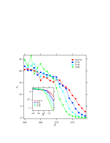
Figure 4: (Color online) The normalized localization length $\Lambda_{N}$ as a function of the energy $E$ around $E\simeq 0.7$ of Fig.3(c) with $D=1.3$ and $W=0.5$. The ensemble size is $2^{12}$. The inset shows the logarithmic plot.

Figure 5: (Color online) The normalized localization length $\Lambda_{N}$ as a function of the energy $E$ at $N=2^{20}$ for $D=1.2,1.3,1.5,1.7$. (a)$W=0.75$, (b)$W=0.5$, (c)$W=0.25$. Note that the data are plotted in logarithmic scale. The black broken lines denote $\Lambda_{N}=1$ as a reference of LDT. The ensemble size is $2^{11}$.

Figure 6: (Color online) The normalized localization length $\Lambda_{N}$ as a function of the energy $E$ with a fixed value of $W=0.25$ for $N=2^{14}\sim 2^{19}$. (a)$D=1.7$, (b)$D=1.5$. Note that the data are plotted in real scales. The ensemble size is $2^{11}$.

Furthermore, it was found that the LDT depends on the value of disorder strength $W$ based on the result in Ref.yamada15 . Figure 5 shows the $E-$dependence of the $\Lambda_{N}$ for some combinations of the disorder strength $W$ and fractal dimension $D$ at the fixed system size of $N=2^{20}$. In the relatively strong disorder cases ($W\geq 0.5$), the delocalized states appear around the band center for $D\leq 3/2$. Figure 6 shows the detail of the $E-$dependence of $\Lambda_{N}$ in the case of $W=0.25$. In the relatively weak disorder case ($W=0.25$), two peaks appear around $|E|\simeq 0.7$ when $D=1.7$ although the states go to localized states with keeping the two-peaks structure of the $E-$dependence for $N\to\infty$, as shown in Fig.6(a). In the case of $D=3/2$, the double-peaks structure of the $E-$dependence remains even for $N\to\infty$, as shown in Fig.6(b). The two peaks revealed ought to influence electronic transport and optical absorption.

3.2 system size dependence:power-law localization

Generally, the quantum states can be classified by the exponent $\delta$ of the $N-$dependence of the $\Lambda_{N}$ when it behaves as,

$$\Lambda_{N}\sim N^{\delta}.$$ (6)

The exponent, $\delta\simeq 0$ for the extended states, $-1<\delta<0$ for the power-law localized states, and $\delta\simeq-1$ for the exponentially localized states. The states at the band center are more delocalized than the states away from the band center.

Figure 7(a) and (b) show the system size dependence of the NLL of a relatively strong disorder case ($W=0.75$) in the vicinity of the band center and edge, respectively. It is found that the $N-$dependence changes the decreasing function with $\delta\simeq-1$ to the constant function $\delta=0$ as the fractal dimension decreases in the case (a). It is found that the critical fractal dimension decreases with increasing the disorder strength, which is consistent with our previous result for $E\neq 0$. On the other hand, the states near band edge are exponentially localized irrespectively of the fractal dimension, as seen in Fig.7 (b).

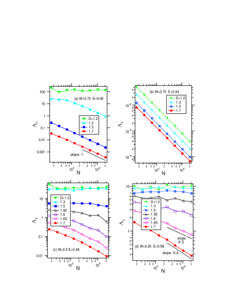
Figure 7: (Color online) The normalized localization length $\Lambda_{N}$ as a function of the system size $N$ with several values of the fractal dimension. (a)$W=0.75,E=0.09$, (b)$W=0.75,E=0.44$ (c)$W=0.5,E=0.48$, (d)$W=0.25,E=0.98$. Note that the data plotted in double-logarithmic scale. The ensemble size is $2^{12}$.

Next, we have to pay attention to the delocalization of the states with energy away from $E=0$ in the relatively weak disorder cases ($W\leqq 0.5$), as given in Fig.7 (c) and (d). Note that the $N-$dependence of the NLL becomes independent of the system size for $D\leq 3/2$ in agreement with the extended nature of the states. The fact that the slopes of the straight lines in the log-log plot are $-1<\delta<0$ strongly suggests the power-law localization of the states. As a result it is suggested that the LDT takes place around the transition point $D_{c}=3/2$ irrespectively of the disorder strength in relatively weak disorder regime $W\leqq 0.5$, as shown in Ref.yamada15 . Exponential localization takes place for $D>3/2$, while the behavior specific for the critical point arises in the whole range of $1<D\leq D_{c}$. In the case of $W<<1$, the latter situation corresponds to the localization with the divergent localization length even for $D>3/2$ and probably should be interpreted as the power-law localization.

4 Distribution of individual normalized localization length and Lyapunov exponent

In this section, we discuss the statistical property of the distribution of individual NLL and Lyapunov exponent at $E=1.0$ that is expected to correpond to a localized state.

First, we define the individual NLL $\Lambda_{N}^{(s)}\equiv 1/(N\gamma_{N}^{(s)})$, where $\gamma_{N}^{(s)}$ is Lyapunov exponent of a finite system with system size $N$ and the suffix $s$ run for each sample. Note that the mean value $\langle\Lambda_{N}^{(s)}\rangle$ satisfies inequality $\Lambda_{N}<\langle\Lambda_{N}^{(s)}\rangle$ because $\langle\gamma_{N}\rangle>1/\langle 1/\gamma_{N}\rangle$. Figure 8 shows the histograms of the distribution of $\Lambda_{N}^{(s)}$ around band edge ($E=1.0$) over $2^{15}$ samples. In the case of $D=1.6$, the asymptotic behavior of the　distribution of $\Lambda_{N}^{(s)}$ gradually moves to the origin position with increasing system size $N$. On the other hand, it is found that in the case of $D=1.5$, it converges the distribution form with power-law tail. The $N-$dependence of the mean value $\langle\Lambda_{N}^{(s)}\rangle$ and the standard deviation $\sigma_{\Lambda}$ are shown in Fig.9. The $N-$dependence is unstable and a clear difference does not appear between the cases of $D=1.6$ and $D=1.5$, different from cases of $\Lambda_{N}$ in the last section.

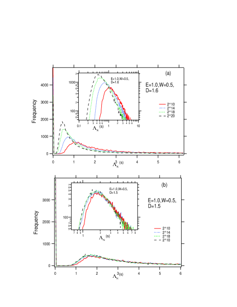
Figure 8: (Color online) Histograms of the distribution of $\Lambda_{N}^{(s)}$ around band edge over $2^{15}$ samples in the cases (a)$D=1.6$ and (b)$D=1.5$. The other parameters are $W=0.5$, $E=1.0$. The details behavior around $\Lambda_{N}^{(s)}\sim 0$ is shown in each inset in the log-log plot. and the mesh of the horizontal line is $5\times 10^{-2}$.

Figure 9: (Color online) Log-log plot of (a)mean $\langle\Lambda_{N}\rangle$ and (b)standard deviation $\sigma_{\Lambda}$ of the distribution in Fig.8 as a function of system size $N$ at $E=1.0$ for fractal dimension $D=1.4,1.5,1.6$.

In localized regime such as $D=1.6$ and $D=1.5$ around the band edge, Lyapunov exponent $\gamma_{N}$ is better than $\Lambda_{N}^{(s)}$ to study the localization property. Fig.10 shows the histogram of the distribution of Lyapunov exponents around band edge ($E=1.0$) over $2^{15}$ samples. Aa a result the two kinds of distribution coexist. One of the two peaks around $\gamma_{N}\simeq 0$ corresponds to the extended states or power-law localized states. Fig.11 shows $N-$dependence of the mean value $\langle\gamma_{N}\rangle$ and standard deviation $\sigma_{\gamma_{N}}$ of the distribution for some cases. We estimate the Lyapunov exponent $\gamma_{\infty}$ for $N\to\infty$ by fitting the relation,

$$\langle\gamma_{N}\rangle=c_{1}N^{-\alpha}+\gamma_{\infty},$$ (7)

for all the cases in Fig.11(a). The estimated parameters are shown in Fig.12. As a result, at least, the Lyapunov exponent becomes zero, $\gamma_{\infty}\simeq 0$, for $D\leq 1.7$ at the band edge ($E=1.0$), which is consistent with power-law localization in the last section.

The distribution form tends to be anomalous around the LDT and the ensemble-averaged value of the finite system size becomes unstable. Accordingly, it is important to investigate the statistical property of the distribution around the transition point because it is sensitive to the difference of the definition, as seen in this section.

Figure 10: (Color online) Histograms of the distribution of $\gamma_{N}$ around band edge ($E=1.0$) in the case of $D=1.6$. The details behavior around $\gamma_{N}\sim 0$ is shown in the inset in the semi-log plot. The ensemble size is $2^{15}$ and the mesh of the horizontal line is $2\times 10^{-7}$.

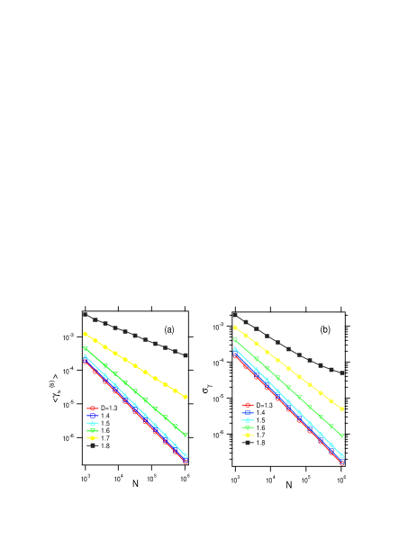
Figure 11: (Color online) Log-log plot of (a)mean $\langle\Lambda_{N}\rangle$ and (b)standard deviation $\sigma_{\Lambda}$ of the distribution in Fig.8 as a function of system size $N$ at $E=1.0$ for fractal dimension $D=1.4,1.5,1.6$. A relation $\langle\gamma_{N}\rangle>\sigma_{\gamma}$ is satisfied and stable.

Figure 12: (Color online) D-dependence of the fitting parameter (a) $\alpha$ and (b)$\gamma(\infty)$ in Eq.(7).

5 Summary and discussion

In summary, we have numerically studied the nature of LDT in 1DDS with fractal disorder generated by Weirstrasse function. We have explicitly shown some basic features of the system. We used the normalized localization length defined by the Lyapunov exponent to investigate the delocalized behavior of the wavefunctions for the entire energy region. The results suggest that in the weak disorder cases a metallic band of extended states in the finite region of the energy exists for $D\simeq 3/2$. In addition, the power-law localized states have been observed for $D\geq 3/2$, with decreasing the fractal dimension $D$ in the cases. On the other hand, the $N-$dependence of the NLL suggests that for the strong disorder cases all the states are exponentially localized even for $1.3<D\lesssim 1.5$, which is consistent with the finding of Ref.yamada15 . We have revealed the anomalous distribution of the individual NLL, as well as found that the asymptotic behaviour of the ensemble-average for Lyapunov exponent $\langle\gamma_{N}\rangle$ consists in that the latter goes to zero with increasing the system’s size for $D\leq 1.7$.

The same properties as in the 1D electronic system given in this paper are also expected for the delocalization of acoustic wave esmailpour08 ; moura11 ; moura15 , electromagnetic wave sheng90 ; diaz05 and seismic wave shahbaz05 in one-dimensional layered media with fractal disorder. We expect that the present work would stimulate further studies of the localization-delocalization transition in 1DDS.

Appendix A potential roughness and eigen functions

The LDT is closely connected to the relation between roughness of the potential landscapes and the degree of differentiability of the potential in the continuum limit greis81 ; garcia09 ; garcia10 ; petersen12 ; petersen13 ; yamada14 It has been proposed that delocalized states can be generated for continuum 1DDS provided that the disorder potential is $V(x)\in C^{\beta}$ with $\beta>1/2$ garcia09 ; garcia10 . The eigenstates are delocalized by properly changing the parameter $L$ which controls the fluctuation of the potential. The singularity of the potential could be regulated by increasing the parameter $L$, as given in Fig.13.

Figure 13: (Color online) Typical on-site energy landscape $WV(n)$ generated by Eq.(2) with $L=2,4,6,8$ and $D=1.7$. A case of $N=2^{10}$ and $W=0.75$ is shown. Notice that ones for $L>10$ can not be distinguishable in this scale.

In Fig.14 the wavefunction absolute values for some eigenstates versus the site index are shown, using rigid boundary condition. It is found that the eigenstates closest to the center of the spectrum tend to be more delocalized than those closer to its edge. In particular, in the case of $L=8$ the eigenstate close to center of the spectrum is localized even for $D=1.7$ as shown in Fig.14(c).

Figure 14: (Color online) Comparison of some eigenstates $|\phi(n)|$ for the cases of $L=2,4,6,8$ in Fig.13 with $D=1.7$ and $W=0.75$. (a)The 1028th energy eigenstates closest to the spectrum edge, (b)the 768th energy eigenstates, (c)the 512th energy eigenstates closest to the spectrum center . Note that the horizontal axis in real scale. Inset of the panel (a) is the logarithmic plot.

References

- (1) K. Ishii, Prog. Theor. Phys. Suppl. 53, 77(1973).
- (2) E. Abrahams, P. W. Anderson, D. C. Licciardello, and T. V. Ramakrishnan, Rhys. Rev.Lett. 42, 673 (1979).
- (3) L.M. Lifshiz, S.A. Gredeskul and L.A. Pastur, Introduction to the theory of Disordered Systems, (Wiley, New York,1988).
- (4) H. Yamada, M. Goda and Y. Aizawa, J. Phys.: Condens. Matter 3, 10043(1991), H.Yamada, Phys. Rev. B 69 014205(2004), H.Yamada, Phys. Lett. A 325 118(2004), H. Yamada, H.Yamada and T.Okabe, Phys. Rev. E 63, 026203(2001).
- (5) C.R. de Oliveira and G.Q. Pellegrino, J. Phys. A 34, L239-L243 (2001).
- (6) R. A. Pinto, M. Rodriguez, J. A. Gonzalez, and E. Medina, Phys. Lett. A 341, 101-106(2005).
- (7) A. Esmailpour, H. Cheraghchi, P. Carpena and M. R. R. Tabar, J. Stat. Mech. P09014(2007).
- (8) M. O. Sales, F. A. B. F. de Moura, Physica E 45, 97-102(2012).
- (9) H. Cheraghchi, S. M. Fazeli, and K. Esfarjani, Phys. Rev. B 72, 174207(2005).
- (10) E. Lazoa, E. Diezb, Phys. Lett. A 374, 3538–3545(2010).
- (11) F.A.B.F.de Moura, and M.L.Lyra, Phys. Rev. Lett. 81 3735(1998).
- (12) F.M.Izrailev and A.A.Krokhin, Phys. Rev. Lett. 82, 4062(1999).
- (13) F. M. Izrailev, A. A. Krokhin, and N. M. Makarov, Phys. Rep. 512, 125 (2012).
- (14) G.-P. Zhang and S.-J. Xionga, Eur. Phys. J. B 29, 491-495(2002).
- (15) H.Shima, T.Nomura and T.Nakayama, Phys. Rev. B 70, 075116(2004).
- (16) T. Kaya, Eur. Phys. J. B 55 (2007) 49.
- (17) T. Kaya, Eur. Phys. J. B 67 (2009) 225.
- (18) L.Y. Gong, P.Q. Tong, and Z.C. Zhou, Eur. Phys. J. B 77, 413-417(2010).
- (19) A. Croy, P. Cain, and M. Schreiber, Eur. Phys. J. B 82, 107 (2011).
- (20) Chao-Sheng Deng, and HuiXu, Physica E 44 1473-1477(2012).
- (21) L. Gong, L. Wei, S. Zhao, and W. Cheng, Phys. Rev. E 86, 061122 (2012).
- (22) C. Albrecht and S. Wimberger, Phys. Rev. B 85, 045107 (2012).
- (23) A. M. Garcia-Garcia, and E. Cuevas, Phys. Rev. B 79, 073104 (2009).
- (24) A. M. Garcia-Garcia, and E. Cuevas, Phys. Rev. B 82, 033412 (2010).
- (25) G.M. Petersen and N. Sandler, arXiv:1206.3370v3 [cond-mat.dis-nn].
- (26) G.M. Petersen and N. Sandler, Phys. Rev. B 87,195443(2013).
- (27) H.S. Yamada, Eur. Phys. J. B 88, 264(2015).
- (28) P. Dean, Rev. Mod. Phys. 44, 127(1972).
- (29) J. J. Ladik, Quantum Theory of Polymers as Solids. (Plenum Press, New Yourk, London 1988).
- (30) Shi-Jie Xiong and S. N. Evangelou, Phys. RevB. 64.113107(2001).
- (31) Igor Travˇenec, physica status solidi b 245, 1604(2008).
- (32) L. Bellando, A. Gero, E. Akkermans, and R. Kaiser, Phys. Rev. A 90, 063822(2014).
- (33) Ayoub Esmailpour, M. Esmailpour, Ameneh Sheikhan, M. Elahi, M. Reza Rahimi Tabar, and Muhammad Sahimi, Phys. Rev. B 78, 134206(2008).
- (34) A.E. Costa, and F.A.B.F. de Moura, J. Phys.: Condens Matter, 23, 065101(2011).
- (35) M. P. S. Junior, M.L. Lyra and F. A. B. F. de Moura, Acta. Phys. Pol. B 46, 1247(2015).
- (36) P. Sheng, Scattering and Localization of Classical Waves in Random Media, (World Scientific, Singapore, 1990).
- (37) E. Diaz, A. Rodriguez, F. Domínguez-Adame and V. A. Malyshev, Europhys. Lett. 72, 1018-1024(2005).
- (38) F. Shahbazi, Alireza Bahraminasab, S. Mehdi Vaez Allaei, Muhammad Sahimi, and M. Reza Rahimi Tabar, Phys. Rev. Lett. 94, 165505(2005).
- (39) N. P. Greis and H. S. Greenside, Phys. Rev. A 44, 2324(1991).
- (40) H.S.Yamada and K.S. Ikeda, Eur. Phys. J. B 87, 208(2014).