Polynomial Diffusion Models for Life Insurance Liabilities

Francesca Biagini111Main affiliation: Department of Mathematics, LMU, Theresienstraße, 39, 80333 Munich, Germany, Email: biagini@math.lmu.de 222Secondary affiliation: Department of Mathematics, University of Oslo, Box 1053, Blindern, 0316, Oslo, Norway.    Yinglin Zhang333Department of Mathematics, LMU, Theresienstraße, 39, 80333 Munich, Germany, Email: zhang@math.lmu.de
(03 August 2016)
Abstract

In this paper we study the pricing and hedging problem of a portfolio of life insurance products under the benchmark approach, where the reference market is modelled as driven by a state variable following a polynomial diffusion on a compact state space. Such a model can be used to guarantee not only the positivity of the OIS short rate and the mortality intensity, but also the possibility of approximating both pricing formula and hedging strategy of a large class of life insurance products by explicit formulas.
 
JEL Classification: C02, G10, G19
 
Key words: life insurance liability, polynomial diffusion, benchmark approach, stochastic mortality intensity, benchmarked risk-minimization.

1 Introduction

The goal of this paper is to analyse the problem of pricing and hedging portfolios of life insurance liabilities under the new approach of combining the benchmark methodology and the existence of a polynomial diffusion state variable which moves on a compact state space and drives the reference market. We consider on the market OIS bonds as well as longevity bonds, both modelled as function of the state variable representing the underlying risk factors, possibly including macro-economic variables, environmental and social indicators. In this way we also introduce a dependence structure between OIS short rate and mortality intensity. Recent studies, see e.g. [35], [13] and [15], confirm the important role of this dependence structure when pricing life insurance liabilities.

The biggest advantage of polynomial diffusions is that they give explicit and tractable formula for conditional expectation of polynomial functions of state variable, see [23]. In our model, we focus in particular on the case when the state variable takes value in a compact state space, which is studied in detail in [32]. Under our model assumptions, the compactness of the state space guarantees the positivity of both OIS short rate and mortality intensity, as well as the possibility of using polynomial approximation for pricing and hedging life insurance liabilities. Nevertheless, the compactness of the state variable implies also the boundedness of OIS short rate and mortality intensity. However, the assumption of bounded short rate is not new to the literature (see e.g. [44], [25], [17], [2], [34] etc.), as well as the assumption of bounded mortality intensity (see e.g. [33]). This last assumption is also supported by recent statistical studies of mortality rates (see e.g. [19] and [31]) and can be understood in terms of confidence region (see [33]).

Unlike [23], we do not assume the existence of a state price density which is equivalent to the existence of a martingale measure. We work under the historical or real world probability measure {\mathbb{P}} and assume only the existence of a benchmark or numéraire portfolio, as proposed by E. Platen (see e.g. [39], [41], [42]). As pointed out by [28], this assumption equals the no unbounded profit with bounded risk condition, which is weaker than the classic risk-neutral condition of no free-lunch with vanishing risk (see e.g. [16]) equivalent to the existence of a martingale measure. The hybrid market composed by both financial and insurance market is intrinsically incomplete due to the presence of additional orthogonal sources of randomness given by the mortality risk. The securitization under the benchmark approach can be resolved by the so called benchmarked risk-minimizing method, see e.g. [40], [42], [20] and [6] for a single payoff. Here we extend the results in [6] of hedging in incomplete markets under the benchmark approach to the case of assets with dividend payments and analyse its relation with the real world pricing formula.

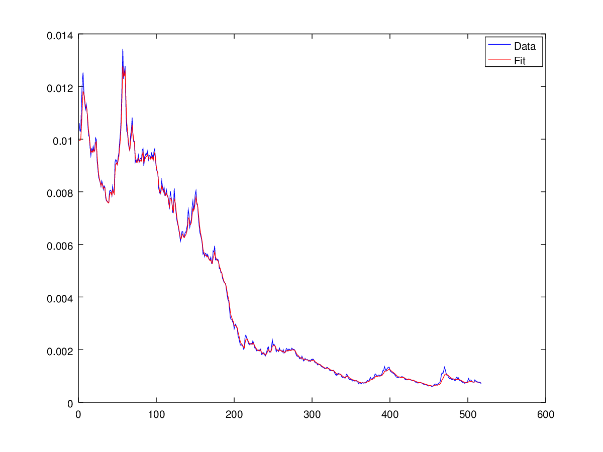
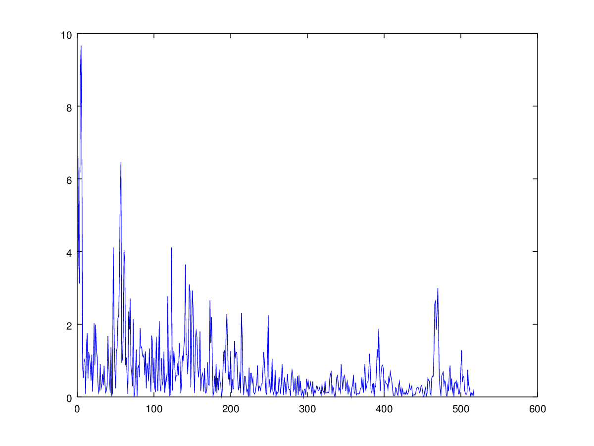
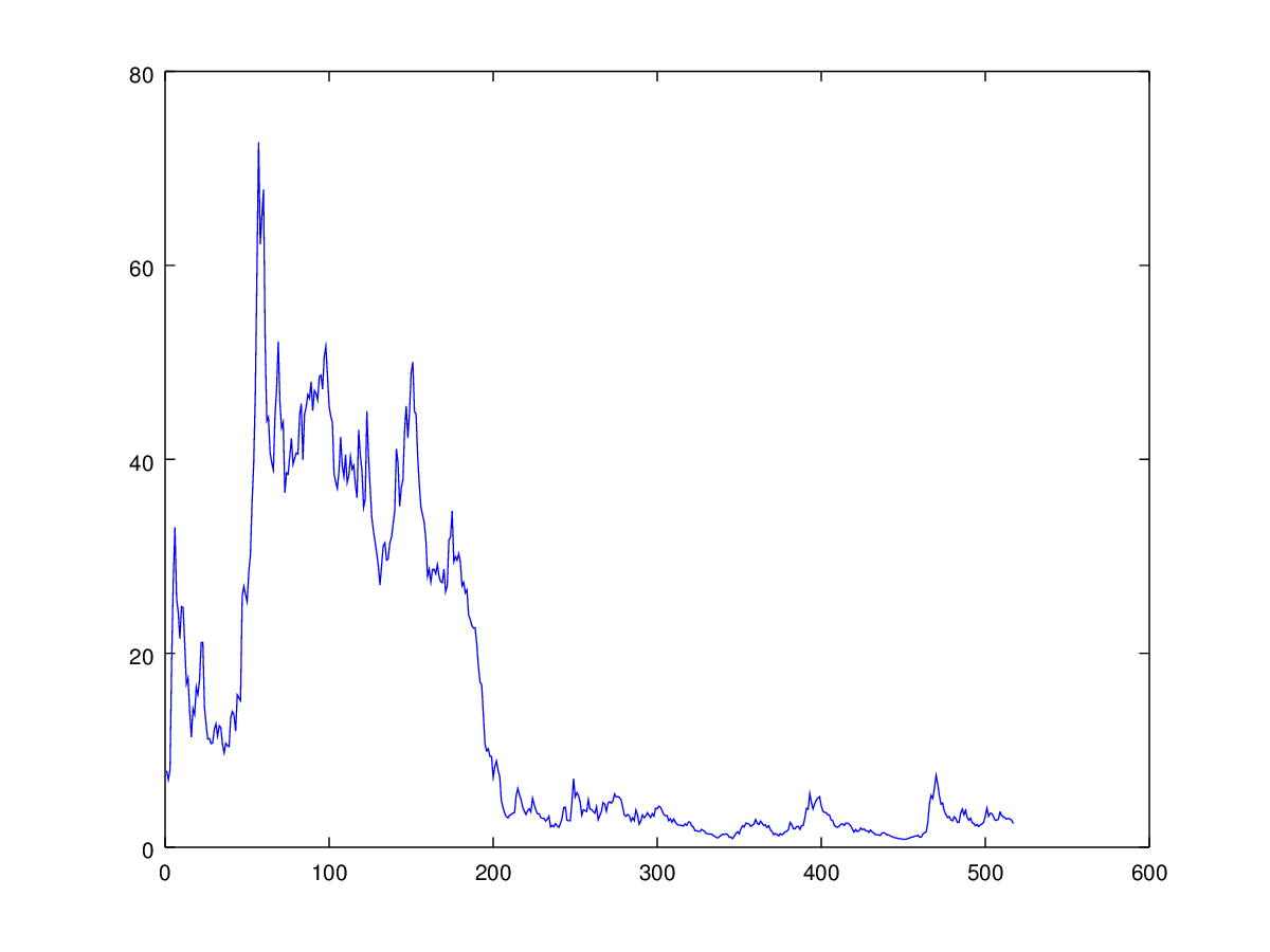
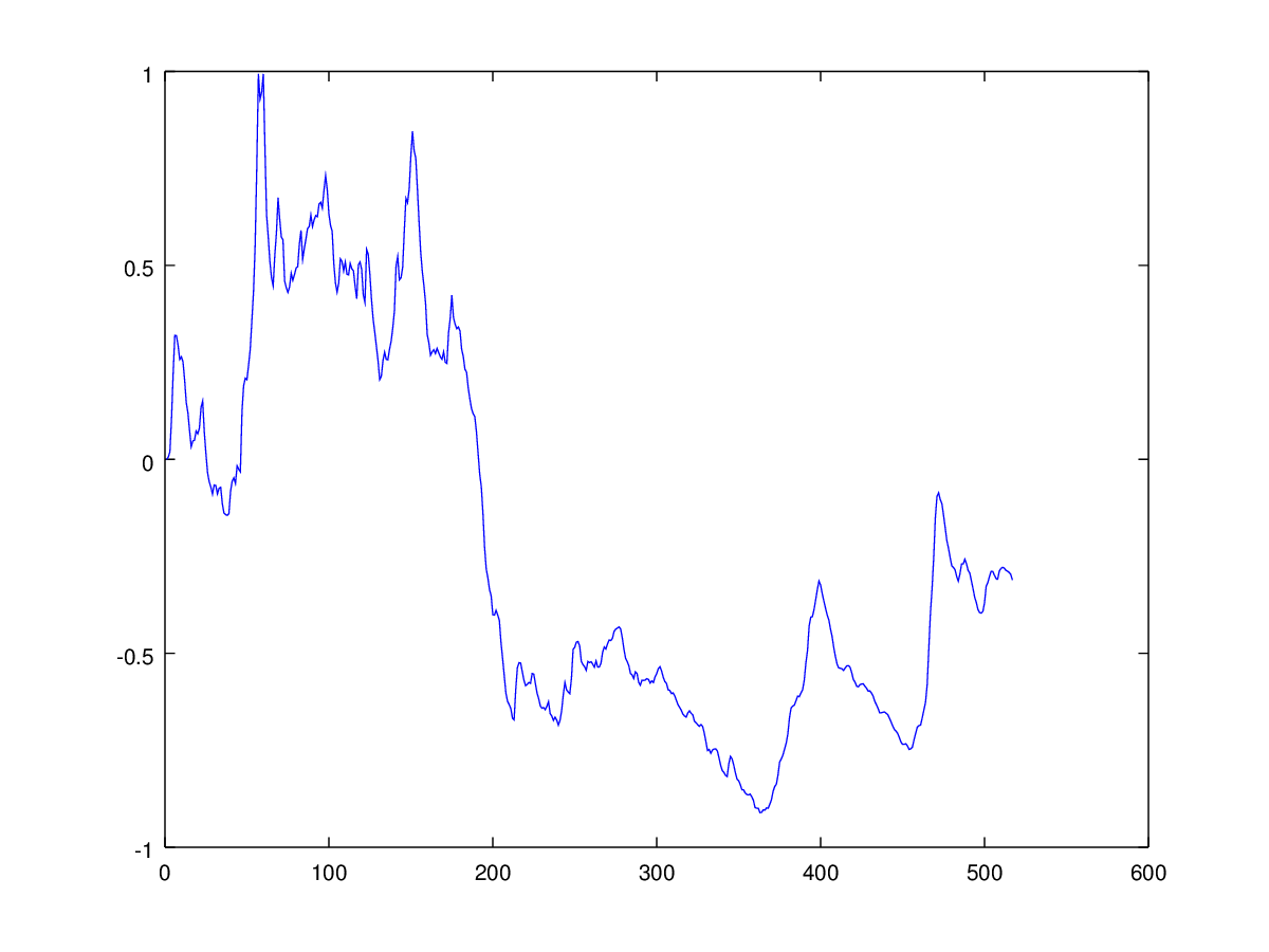
The paper is structured as follows. Section 2 provides a brief introduction of polynomial diffusions. Section 3 gives the basic model structure assumptions for a portfolio of life insurance policies under the intensity-based approach. A benchmark portfolio is assumed to exist. Benchmark portfolio, OIS bond and longevity bond are then modelled explicitly in terms of a possibly multi-dimensional state variable which follows a polynomial diffusion on a compact state space. The real world pricing formula is provided explicitly in Section 4 for all three building blocks of insurance products (pure endowment, term insurance, annuity) in the case of payoff given by polynomial functions of the state variable. We then show how these explicit results can be used to approximate more general forms of payment process. For the sake of simplicity, we derive explicitly the benchmarked risk-minimizing strategy and its polynomial approximation only for pure endowment contracts, since the other two cases are similar. In Section 5 we use a 2-dimensional state variable and calibrate our model to MSCI and LLMA index under linear specification of the inverse of benchmark and the longevity index. We show how this parsimonious specification can already produce a good fit to market data. In Appendix A we extend the real world pricing formula and the benchmarked risk-minimizing method to dividend payments and discuss their relationship.

2 Polynomial diffusion

In this section, we give a synthetic overview of the most important results for polynomial diffusions which will be used to model our market. For details about these processes, see [23].

Let Ed𝐸superscript𝑑E\subset{\mathbb{R}}^{d} be a compact set with non-empty internal part, called state space. Let 𝕊dsuperscript𝕊𝑑{\mathbb{S}}^{d} denote the space of real symmetric d×d𝑑𝑑d\times d matrices, and 𝕊+dsubscriptsuperscript𝕊𝑑{\mathbb{S}}^{d}_{+} the convex cone of positive semidefinite symmetric matrices. For a given n𝑛n\in\mathbb{N}, we denote furthermore by Poln(E)subscriptPol𝑛𝐸{\text{Pol}_{n}(E)} the following finite-dimensional vector space

Poln(E):={polynomials on E of degree n},assignsubscriptPol𝑛𝐸polynomials on E of degree n{\text{Pol}_{n}(E)}:=\{\text{polynomials on $E$ of degree $\leqslant n$}\},

and by Nnsubscript𝑁𝑛N_{n} the dimension of Poln(E)subscriptPol𝑛𝐸{\text{Pol}_{n}(E)}. We consider a fixed time horizon [0,T]0𝑇[0,T] and an E𝐸E-valued process Z:=(Zt)t[0,T]assign𝑍subscriptsubscript𝑍𝑡𝑡0𝑇Z:=(Z_{t})_{t\in[0,T]}, with the following dynamics

dZt=b(Zt)dt+σ(Zt)dWt,dsubscript𝑍𝑡𝑏subscript𝑍𝑡d𝑡𝜎subscript𝑍𝑡dsubscript𝑊𝑡\mathrm{d}Z_{t}=b(Z_{t})\mathrm{d}t+\sigma(Z_{t})\mathrm{d}W_{t}, (2.1)

realized on a filtered probability space (Ω,,𝔽,)Ω𝔽(\Omega,{\mathcal{F}},{\mathbb{F}},{\mathbb{P}}), with 𝔽:=(t)t[0,T]assign𝔽subscriptsubscript𝑡𝑡0𝑇{\mathbb{F}}:=({\mathcal{F}}_{t})_{t\in[0,T]}. W:=(Wt)t[0,T]assign𝑊subscriptsubscript𝑊𝑡𝑡0𝑇W:=(W_{t})_{t\in[0,T]} is a d𝑑d-dimensional 𝔽𝔽{\mathbb{F}}-Brownian motion, σ:dd×d:𝜎superscript𝑑superscript𝑑𝑑\sigma:{\mathbb{R}}^{d}\rightarrow{\mathbb{R}}^{d\times d} is a continuous function, a:=σσassign𝑎𝜎superscript𝜎top{a}:={\sigma}{\sigma}^{\top}, a𝑎{a} and b𝑏{b} are two fixed maps

a:d𝕊d,b:dd,:𝑎superscript𝑑superscript𝕊𝑑𝑏:superscript𝑑superscript𝑑{a}:{\mathbb{R}}^{d}\rightarrow{\mathbb{S}}^{d},\ \ \ \ {b}:{\mathbb{R}}^{d}\rightarrow{\mathbb{R}}^{d},

such that

aij|EPol2(E),bi|EPol1(E),formulae-sequenceevaluated-atsubscript𝑎𝑖𝑗𝐸subscriptPol2𝐸evaluated-atsubscript𝑏𝑖𝐸subscriptPol1𝐸\left.{a}_{ij}\right|_{E}\in\text{Pol}_{2}(E),\ \ \ \ \left.{b}_{i}\right|_{E}\in\text{Pol}_{1}(E), (2.2)

for all i,j=1,,dformulae-sequence𝑖𝑗1𝑑i,j=1,...,d. The initial value Z0subscript𝑍0Z_{0} is assumed to be constant and belonging to E𝐸E.

We consider the following operator 𝐆𝐆\mathbf{G} associated to the process Z𝑍Z

𝐆:𝒞2(d),:𝐆superscript𝒞2superscript𝑑\mathbf{G}:\mathcal{C}^{2}({\mathbb{R}}^{d})\longrightarrow{\mathbb{R}},

defined by

𝐆f(z):=12Tr(a(z)2f(z))+b(z)f(z),zd.formulae-sequenceassign𝐆𝑓𝑧12Tr𝑎𝑧superscript2𝑓𝑧𝑏superscript𝑧top𝑓𝑧𝑧superscript𝑑\mathbf{G}f(z):=\frac{1}{2}\text{Tr}({a}(z)\nabla^{2}f(z))+{b}(z)^{\top}\nabla f(z),\ \ \ \ z\in{\mathbb{R}}^{d}. (2.3)
Definition 2.1.

An E𝐸E-valued process Z𝑍Z satisfying (2.1) is called a polynomial diffusion on E𝐸E if

𝐆Poln(E)Poln(E),for all n.formulae-sequence𝐆subscriptPol𝑛𝐸subscriptPol𝑛𝐸for all 𝑛\mathbf{G}{\text{Pol}_{n}(E)}\subseteq{\text{Pol}_{n}(E)},\ \ \ \ \text{for all }\ \ n\in{\mathbb{N}}.

Lemma 2.2 of [23] shows that Z𝑍Z is a polynomial diffusion on E𝐸E if and only if (2.2) holds. In such case, for every fixed n𝑛n\in{\mathbb{N}}, its associated operator 𝐆𝐆\mathbf{G} admits a unique matrix representation GnNn×Nnsubscript𝐺𝑛superscriptsubscript𝑁𝑛subscript𝑁𝑛G_{n}\in{\mathbb{R}}^{N_{n}\times N_{n}} restricted to Poln(E)subscriptPol𝑛𝐸{\text{Pol}_{n}(E)}. That is, for each pPoln(E)𝑝subscriptPol𝑛𝐸p\in{\text{Pol}_{n}(E)} with coordinate representation

p(z)=Hn(z)p,zd,formulae-sequence𝑝𝑧subscript𝐻𝑛superscript𝑧top𝑝𝑧superscript𝑑p(z)=H_{n}(z)^{\top}\vec{p},\ \ \ \ z\in{\mathbb{R}}^{d}, (2.4)

where Hn(z)subscript𝐻𝑛𝑧H_{n}(z) is a fixed basis vector of Poln(E)subscriptPol𝑛𝐸{\text{Pol}_{n}(E)} and pNn𝑝superscriptsubscript𝑁𝑛\vec{p}\in{\mathbb{R}}^{N_{n}}, we have

𝐆p(z)=Hn(z)Gnp,zd.formulae-sequence𝐆𝑝𝑧subscript𝐻𝑛superscript𝑧topsubscript𝐺𝑛𝑝𝑧superscript𝑑\mathbf{G}p(z)=H_{n}(z)^{\top}G_{n}\vec{p},\ \ \ \ z\in{\mathbb{R}}^{d}.

The following proposition gives one of the most important results for polynomial diffusions: the 𝔽𝔽{\mathbb{F}}-martingale generated by a polynomial function of ZTsubscript𝑍𝑇Z_{T} is again given by a polynomial function of the state variable with deterministic time-dependent coefficients.

Proposition 2.2 (Polynomial conditional expectation).

Let n𝑛n\in{\mathbb{N}}, pPoln(E)𝑝subscriptPol𝑛𝐸p\in{\text{Pol}_{n}(E)} with coordinate representation (2.4) and 0tT0𝑡𝑇0\leqslant t\leqslant T. If Z𝑍Z is a E𝐸E-solution to (2.1), then

𝔼[p(ZT)|t]=Hn(Zt)e(Tt)Gnp.𝔼delimited-[]conditional𝑝subscript𝑍𝑇subscript𝑡subscript𝐻𝑛superscriptsubscript𝑍𝑡topsuperscript𝑒𝑇𝑡subscript𝐺𝑛𝑝\mathbb{E}\left[\left.p(Z_{T})\right|{\mathcal{F}}_{t}\right]=H_{n}(Z_{t})^{\top}e^{(T-t)G_{n}}\vec{p}. (2.5)
Proof.

See Theorem 3.1 of [23]. ∎

For the sake of simplicity, we introduce the notation

p^(t,T)(Zt):=Hn(Zt)e(Tt)Gnp,t[0,T].formulae-sequenceassignsubscript^𝑝𝑡𝑇subscript𝑍𝑡subscript𝐻𝑛superscriptsubscript𝑍𝑡topsuperscript𝑒𝑇𝑡subscript𝐺𝑛𝑝𝑡0𝑇\hat{p}_{(t,T)}(Z_{t}):=H_{n}(Z_{t})^{\top}e^{(T-t)G_{n}}\vec{p},\ \ \ \ t\in[0,T].

The following two theorems give some sufficient conditions on the state space E𝐸E, under which an E𝐸E-valued state variable Z𝑍Z admits weak uniqueness and existence.

Theorem 2.3.

Let Z𝑍Z be an E𝐸E-valued solution to (2.1). If E𝐸E is compact, then Z𝑍Z is weakly unique, i.e. any other E𝐸E-valued solution to (2.1) with initial value Z0subscript𝑍0Z_{0} has the same law as Z𝑍Z.

Proof.

See Theorem 5.1 of [23]. ∎

Remark 2.4.

For d=1𝑑1d=1, we have also strong uniqueness (or pathwise uniqueness) for a E𝐸E-valued solution to (2.1), see [43]. Further discussion about the strong uniqueness for a generic dimension is provided in [32].

Theorem 2.5.

Let 𝒫𝒫\mathcal{P} be a family of polynomials on dsuperscript𝑑{\mathbb{R}}^{d}. If the boundary of the state space E𝐸E is defined by these polynomials, i.e.

E={xd:p(x)0 for all p𝒫},𝐸conditional-set𝑥superscript𝑑𝑝𝑥0 for all 𝑝𝒫E=\{x\in{\mathbb{R}}^{d}:p(x)\leqslant 0\text{ for all }p\in\mathcal{P}\},

then the following conditions on the parameters a𝑎a and b𝑏b guarantee the existence of an E𝐸E-valued solution to (2.1):

  1. 1.

    a𝕊+d𝑎subscriptsuperscript𝕊𝑑a\in{\mathbb{S}}^{d}_{+};

  2. 2.

    ap=0𝑎𝑝0a\nabla p=0 on {p=0}𝑝0\{p=0\} for each p𝒫𝑝𝒫p\in\mathcal{P};

  3. 3.

    𝐆p>0𝐆𝑝0\mathbf{G}p>0 on E{p=0}𝐸𝑝0E\cap\{p=0\} for each p𝒫𝑝𝒫\ p\in\mathcal{P}.

Proof.

This theorem is a simplified version of Theorem 5.3 of [23]. ∎

Remark 2.6.

We stress that every E𝐸E-solution to (2.1) is a strong Markov process thanks to the compactness of the state space and the weak uniqueness given by Theorem 2.3 (see e.g. Theorem 4.6 of [22]). The operator defined in (2.3) is thus the extended Markov generator of Z𝑍Z.

3 The Setting

In this paper, we follow the intensity-based reduced-form approach (e.g. [10]) in order to describe life insurance derivatives linked to a portfolio of life insurance contracts.

We fix a finite time horizon [0,T]0𝑇[0,T] with 0<T<0𝑇0<T<\infty and a filtered probability space (Ω,𝒢,𝔾,)Ω𝒢𝔾(\Omega,{\mathcal{G}},{\mathbb{G}},{\mathbb{P}}), with 𝔾:=(𝒢t)t[0,T]assign𝔾subscriptsubscript𝒢𝑡𝑡0𝑇{\mathbb{G}}:=({\mathcal{G}}_{t})_{t\in[0,T]}, 𝒢=𝒢T,𝒢0trivial𝒢subscript𝒢𝑇subscript𝒢0trivial{\mathcal{G}}={\mathcal{G}}_{T},{\mathcal{G}}_{0}\ \text{trivial}. The filtration 𝔾𝔾{\mathbb{G}} represents all the information flow available to the insurance company. {\mathbb{P}} is interpreted as the historical or real world probability measure. We consider a life insurance portfolio with n𝑛n policyholders (n𝑛n\in{\mathbb{N}}). For i=1,,n𝑖1𝑛i=1,...,n, the decease time of i𝑖i-th insured person is assumed to be a 𝒢𝒢{\mathcal{G}}-measurable random time τi:(Ω,𝒢,)+:superscript𝜏𝑖Ω𝒢subscript\tau^{i}:(\Omega,{\mathcal{G}},{\mathbb{P}})\rightarrow{\mathbb{R}}_{+}, , such that τi>0superscript𝜏𝑖0\tau^{i}>0 a.s., (τi=0)=0superscript𝜏𝑖00\mathbb{P}(\tau^{i}=0)=0 and (τi>t)>0superscript𝜏𝑖𝑡0{\mathbb{P}}(\tau^{i}>t)>0 for any t[0,T]𝑡0𝑇t\in[0,T]. These last conditions mean that the decease of a policyholder does not occur in the first instant and may never occur during the considered time horizon [0,T]0𝑇[0,T]. We denote the death counting process by N:=(Nt)t[0,T]assign𝑁subscriptsubscript𝑁𝑡𝑡0𝑇N:=(N_{t})_{t\in[0,T]},

Nt=i=1n𝟏{τit},t[0,T].formulae-sequencesubscript𝑁𝑡superscriptsubscript𝑖1𝑛subscript1superscript𝜏𝑖𝑡𝑡0𝑇N_{t}=\sum_{i=1}^{n}\mathbf{1}_{\left\{\tau^{i}\leqslant t\right\}},\ \ \ \ t\in[0,T]. (3.1)

Furthermore, we assume 𝔾=𝔽1n𝔾𝔽superscript1superscript𝑛{\mathbb{G}}={\mathbb{F}}\vee{\mathbb{H}}^{1}\vee...\vee{\mathbb{H}}^{n} where for i=1,,n𝑖1𝑛i=1,...,n, i:=(ti)t[0,T]assignsuperscript𝑖subscriptsubscriptsuperscript𝑖𝑡𝑡0𝑇{\mathbb{H}}^{i}:=({\mathcal{H}}^{i}_{t})_{t\in[0,T]}, 𝔽:=(t)t[0,T]assign𝔽subscriptsubscript𝑡𝑡0𝑇{\mathbb{F}}:=({\mathcal{F}}_{t})_{t\in[0,T]}, 0=0i=𝒢0={,Ω}subscript0subscriptsuperscript𝑖0subscript𝒢0Ω{\mathcal{F}}_{0}={\mathcal{H}}^{i}_{0}={\mathcal{G}}_{0}=\{\emptyset,\Omega\}, 𝒢=𝒢T=TT1Tn𝒢subscript𝒢𝑇subscript𝑇superscriptsubscript𝑇1superscriptsubscript𝑇𝑛{\mathcal{G}}={\mathcal{G}}_{T}={\mathcal{F}}_{T}\vee{\mathcal{H}}_{T}^{1}\vee...\vee{\mathcal{H}}_{T}^{n}. The filtration 𝔽𝔽{\mathbb{F}} is called reference filtration. For each i=1,,n𝑖1𝑛i=1,...,n, the filtration isuperscript𝑖{\mathbb{H}}^{i} is generated by the jump process of τisuperscript𝜏𝑖\tau^{i} defined by Hi:=(Hti)t[0,T]assignsuperscript𝐻𝑖subscriptsubscriptsuperscript𝐻𝑖𝑡𝑡0𝑇H^{i}:=(H^{i}_{t})_{t\in[0,T]} with Hti=𝟏{τit}subscriptsuperscript𝐻𝑖𝑡subscript1superscript𝜏𝑖𝑡H^{i}_{t}=\mathbf{1}_{\{\tau^{i}\leqslant t\}} for every t[0,T]𝑡0𝑇t\in[0,T], i.e. the filtration isuperscript𝑖{\mathbb{H}}^{i} represents the information through time relative to i𝑖i-th policyholder’s life status described by τisuperscript𝜏𝑖\tau^{i}. All the filtrations are assumed to be complete and right-continuous. Every random variable τisuperscript𝜏𝑖\tau^{i} for i=1,,n𝑖1𝑛i=1,...,n is clearly a 𝔾𝔾{\mathbb{G}}-stopping time, but not necessary an 𝔽𝔽{\mathbb{F}}-stopping time. We assume also that for each i,j=1,,nformulae-sequence𝑖𝑗1𝑛i,j=1,...,n, (τi=τj)=0superscript𝜏𝑖superscript𝜏𝑗0\mathbb{P}\left(\tau^{i}=\tau^{j}\right)=0 and that τisuperscript𝜏𝑖\tau^{i} and τjsuperscript𝜏𝑗\tau^{j} are 𝔽𝔽{\mathbb{F}}-conditionally independent, i.e. for any t[0,T]𝑡0𝑇t\in[0,T] and s,r[0,t]𝑠𝑟0𝑡s,r\in[0,t],

(τi>s,τj>r|t)=(τi>s|t)(τj>r|t).formulae-sequencesuperscript𝜏𝑖𝑠superscript𝜏𝑗conditional𝑟subscript𝑡superscript𝜏𝑖conditional𝑠subscript𝑡superscript𝜏𝑗conditional𝑟subscript𝑡{\mathbb{P}}\left.\left(\tau^{i}>s,\tau^{j}>r\right|{\mathcal{F}}_{t}\right)={\mathbb{P}}\left.\left(\tau^{i}>s\right|{\mathcal{F}}_{t}\right){\mathbb{P}}\left.\left(\tau^{j}>r\right|{\mathcal{F}}_{t}\right).

This assumption can be interpreted in the following way. The life status of policyholders is influenced by some common systematic factors related to environmental, economic, social and financial conditions captured by the information flow represented by 𝔽𝔽{\mathbb{F}}, but every policyholder has also his own purely individual or idiosyncratic decease factors (e.g. illness, accident etc.).
Moreover, we assume that

  1. 1.

    The subfiltration 𝔽𝔽{\mathbb{F}} of 𝔾𝔾{\mathbb{G}} satisfies the so called H𝐻H-hypothesis, i.e. every 𝔽𝔽{\mathbb{F}}-martingale is also a 𝔾𝔾{\mathbb{G}}-martingale.

  2. 2.

    For every i=1,,n𝑖1𝑛i=1,...,n, the following non-negative 𝔽𝔽{\mathbb{F}}-submartingale Fi:=(Fti)t[0,T]assignsuperscript𝐹𝑖subscriptsubscriptsuperscript𝐹𝑖𝑡𝑡0𝑇F^{i}:=(F^{i}_{t})_{t\in[0,T]}, called conditional cumulative distribution function of τisuperscript𝜏𝑖\tau^{i}

    Fti:=(τit|t),t[0,T]formulae-sequenceassignsubscriptsuperscript𝐹𝑖𝑡superscript𝜏𝑖conditional𝑡subscript𝑡𝑡0𝑇F^{i}_{t}:={\mathbb{P}}\left.\left(\tau^{i}\leqslant t\right|{\mathcal{F}}_{t}\right),\ \ \ \ t\in[0,T]

    satisfies

    Fti<1,t[0,T],formulae-sequencesubscriptsuperscript𝐹𝑖𝑡1𝑡0𝑇F^{i}_{t}<1,\ \ \ \ t\in[0,T],

    and is absolutely continuous with respect to Lebesgue’s measure.

For every i=1,,n𝑖1𝑛i=1,...,n, the hazard process Γi:=(Γti)t[0,T]assignsuperscriptΓ𝑖subscriptsubscriptsuperscriptΓ𝑖𝑡𝑡0𝑇\Gamma^{i}:=(\Gamma^{i}_{t})_{t\in[0,T]} of τisuperscript𝜏𝑖\tau^{i}

Γti:=ln(1Fti),t[0,T]formulae-sequenceassignsubscriptsuperscriptΓ𝑖𝑡1subscriptsuperscript𝐹𝑖𝑡𝑡0𝑇\Gamma^{i}_{t}:=-\ln\left(1-F^{i}_{t}\right),\ \ \ \ t\in[0,T]

is well defined, absolutely continuous and increasing (see Lemma 6.1.2 of [10]). On one hand, this implies that, for every i=1,,n𝑖1𝑛i=1,...,n, τisuperscript𝜏𝑖\tau^{i} avoids all 𝔽𝔽{\mathbb{F}}-stopping times and is a 𝔾𝔾{\mathbb{G}}-totally inaccessible stopping time (see [18]). On the other hand, the absolute continuity of ΓisuperscriptΓ𝑖\Gamma^{i} implies the existence of a non negative 𝔽𝔽{\mathbb{F}}-progressively measurable mortality intensity μi:=(μt)t[0,T]assignsuperscript𝜇𝑖subscriptsubscript𝜇𝑡𝑡0𝑇\mu^{i}:=(\mu_{t})_{t\in[0,T]} with integrable sample paths such that

Γti=0tμuidu,t[0,T].formulae-sequencesubscriptsuperscriptΓ𝑖𝑡superscriptsubscript0𝑡subscriptsuperscript𝜇𝑖𝑢differential-d𝑢𝑡0𝑇\Gamma^{i}_{t}=\int_{0}^{t}\mu^{i}_{u}\mathrm{d}u,\ \ \ \ t\in[0,T].

We can take a 𝔽𝔽{\mathbb{F}}-predictable version of μisuperscript𝜇𝑖\mu^{i}, see Lemma 1.36 of [29]. For the sake of simplicity, we assume a homogeneous insurance portfolio where all policyholders have the same mortality rate and we denote the common conditional cumulative distribution function, hazard process and mortality intensity respectively by F:=(Ft)t[0.T]assign𝐹subscriptsubscript𝐹𝑡𝑡delimited-[]formulae-sequence0𝑇F:=(F_{t})_{t\in[0.T]}, Γ:=(Γt)t[0,T]assignΓsubscriptsubscriptΓ𝑡𝑡0𝑇\Gamma:=(\Gamma_{t})_{t\in[0,T]} and μ:=(μt)t[0,T]assign𝜇subscriptsubscript𝜇𝑡𝑡0𝑇\mu:=(\mu_{t})_{t\in[0,T]}, i.e. F=Fi𝐹superscript𝐹𝑖F=F^{i}, Γ=ΓiΓsuperscriptΓ𝑖\Gamma=\Gamma^{i}, μ=μi𝜇superscript𝜇𝑖\mu=\mu^{i} for all i=1,,n𝑖1𝑛i=1,...,n. This happens for example when all policyholders belong to the same age cohort in the same country444The number of the reference population group is normally much bigger than n𝑛n.. We assume furthermore that there is a publicly accessible index based on mortality data of the given age group. According to [12], such index is modelled by the process I:=(It)t[0,T]assign𝐼subscriptsubscript𝐼𝑡𝑡0𝑇I:=(I_{t})_{t\in[0,T]}, where

It:=1Ft=eΓt=e0tμudu,t[0,T],formulae-sequenceassignsubscript𝐼𝑡1subscript𝐹𝑡superscript𝑒subscriptΓ𝑡superscript𝑒subscriptsuperscript𝑡0subscript𝜇𝑢differential-d𝑢𝑡0𝑇I_{t}:=1-F_{t}=e^{-\Gamma_{t}}=e^{-\int^{t}_{0}\mu_{u}\mathrm{d}u},\ \ \ \ t\in[0,T],

and is called survival index (or longevity index or longevity process) related to the given group of people555The assumption of a homogeneous portfolio can be easily relaxed and extended to the case of more population groups, subdivided by age cohorts, countries etc.. In that case, every group of people is assumed to have its correspondent longevity index and mortality intensity.. We stress that under our assumptions, the reference filtration gives information about the (common) mortality intensity μ𝜇\mu, or equivalently the longevity index I𝐼I, but not about a single decease event itself. For i=1,,n𝑖1𝑛i=1,...,n, we introduce the process Li:=(Lti)t[0,T]assignsuperscript𝐿𝑖subscriptsubscriptsuperscript𝐿𝑖𝑡𝑡0𝑇L^{i}:=(L^{i}_{t})_{t\in[0,T]} associated to the i𝑖i-th policyholder

Lti:=(1Hti)eΓt=𝟏{τi>t}e0tμsds,t[0,T].formulae-sequenceassignsubscriptsuperscript𝐿𝑖𝑡1subscriptsuperscript𝐻𝑖𝑡superscript𝑒subscriptΓ𝑡subscript1superscript𝜏𝑖𝑡superscript𝑒subscriptsuperscript𝑡0subscript𝜇𝑠differential-d𝑠𝑡0𝑇L^{i}_{t}:=(1-H^{i}_{t})e^{\Gamma_{t}}=\mathbf{1}_{\left\{\tau^{i}>t\right\}}e^{\int^{t}_{0}\mu_{s}\mathrm{d}s},\ \ \ \ t\in[0,T]. (3.2)

Proposition 5.7 and Proposition 5.8 of [4] show that Lisuperscript𝐿𝑖L^{i} is a 𝔾𝔾{\mathbb{G}}-martingale and satisfies

Lti=1]0,t]LuidMui,t[0,T],L^{i}_{t}=1-\int_{]0,t]}L^{i}_{u-}\mathrm{d}M^{i}_{u},\ \ \ \ t\in[0,T],

where Mi:=(Mti)t[0,T]assignsuperscript𝑀𝑖subscriptsubscriptsuperscript𝑀𝑖𝑡𝑡0𝑇M^{i}:=(M^{i}_{t})_{t\in[0,T]} is a 𝔾𝔾{\mathbb{G}}-martingale defined by

Mti=HtiΓtτii,t[0,T].formulae-sequencesuperscriptsubscript𝑀𝑡𝑖subscriptsuperscript𝐻𝑖𝑡subscriptsuperscriptΓ𝑖𝑡superscript𝜏𝑖𝑡0𝑇M_{t}^{i}=H^{i}_{t}-\Gamma^{i}_{t\wedge\tau^{i}},\ \ \ \ t\in[0,T].

Hence, (Γtτi)t[0,T]subscriptsubscriptΓ𝑡superscript𝜏𝑖𝑡0𝑇(\Gamma_{t\wedge\tau^{i}})_{t\in[0,T]} is the 𝔾𝔾{\mathbb{G}}-compensator of Hisuperscript𝐻𝑖H^{i}. In other words, the hazard process ΓisuperscriptΓ𝑖\Gamma^{i} coincides up to τisuperscript𝜏𝑖\tau^{i} with the so called (𝔽,𝔾)𝔽𝔾({\mathbb{F}},{\mathbb{G}})-martingale hazard process Λi:=(Λti)t[0,T]assignsuperscriptΛ𝑖subscriptsubscriptsuperscriptΛ𝑖𝑡𝑡0𝑇\Lambda^{i}:=\left(\Lambda^{i}_{t}\right)_{t\in[0,T]} of τisuperscript𝜏𝑖\tau^{i}. Under the assumption of a homogeneous insurance portfolio, if we define the 𝔾𝔾{\mathbb{G}}-martingale M:=(Mt)t[0,T]assign𝑀subscriptsubscript𝑀𝑡𝑡0𝑇M:=(M_{t})_{t\in[0,T]} as

M:=i=1nMi,assign𝑀superscriptsubscript𝑖1𝑛superscript𝑀𝑖M:=\sum_{i=1}^{n}M^{i},

then

Mt=Nt(nNt)Γt,t[0,T],formulae-sequencesubscript𝑀𝑡subscript𝑁𝑡𝑛subscript𝑁limit-from𝑡subscriptΓ𝑡𝑡0𝑇M_{t}=N_{t}-(n-N_{t-})\Gamma_{t},\ \ \ \ t\in[0,T], (3.3)

i.e. the 𝔾𝔾{\mathbb{G}}-compensator of the death counting process N𝑁N is given by ((nNt)Γt)t[0,T]subscript𝑛subscript𝑁limit-from𝑡subscriptΓ𝑡𝑡0𝑇\left((n-N_{t-})\Gamma_{t}\right)_{t\in[0,T]}.

3.1 Market model

We assume that our reference market is frictionless and there are l𝑙l liquidly traded primary assets with price processes Si:=(Sti)t[0,T]assignsuperscript𝑆𝑖subscriptsubscriptsuperscript𝑆𝑖𝑡𝑡0𝑇S^{i}:=(S^{i}_{t})_{t\in[0,T]}, i=1,,l𝑖1𝑙i=1,...,l, following real-valued continuous (,𝔽)𝔽({\mathbb{P}},{\mathbb{F}})-semimartingales. The asset vector is denoted by S:=(Si)i=1,,lassign𝑆subscriptsuperscript𝑆𝑖𝑖1𝑙S:=(S^{i})_{i=1,...,l}. For now we do not specify the nature and the dynamics of these primary assets.

Remark 3.1.

We remark that primary assets are here assumed to be 𝔽𝔽{\mathbb{F}}-adapted. Unlike in the credit risk context where products associated to a single default (e.g. bankruptcy of an important finance institution) are traded on the financial market over time, this is not the case of life insurance products based on the decease of single persons. However, primary assets can include some mortality/longevity index-linked securities, like longevity bond.

Definition 3.2.

A trading strategy is a lsuperscript𝑙{\mathbb{R}}^{l}-valued 𝔾𝔾{\mathbb{G}}-predictable S𝑆S-integrable process δ:=(δt)t[0,T]assign𝛿subscriptsubscript𝛿𝑡𝑡0𝑇\delta:=(\delta_{t})_{t\in[0,T]}.

The space of all lsuperscript𝑙{\mathbb{R}}^{l}-valued 𝔾𝔾{\mathbb{G}}-predictable S𝑆S-integrable processes is indicated by L(S,,𝔾)𝐿𝑆𝔾L(S,{\mathbb{P}},{\mathbb{G}}).

Definition 3.3.

A portfolio or value process Sδ:=(Stδ)t[0,T]assignsuperscript𝑆𝛿subscriptsubscriptsuperscript𝑆𝛿𝑡𝑡0𝑇S^{\delta}:=(S^{\delta}_{t})_{t\in[0,T]} associated to a trading strategy δ𝛿\delta is defined by the following càdlàg optional process666We follow the definition given in [7].

Stδ=δtSt=i=1lδtiSti,t[0,T].formulae-sequencesubscriptsuperscript𝑆𝛿limit-from𝑡superscriptsubscript𝛿𝑡topsubscript𝑆𝑡superscriptsubscript𝑖1𝑙subscriptsuperscript𝛿𝑖𝑡subscriptsuperscript𝑆𝑖𝑡𝑡0𝑇S^{\delta}_{t-}=\delta_{t}^{\top}S_{t}=\sum_{i=1}^{l}\delta^{i}_{t}S^{i}_{t},\ \ \ \ t\in[0,T].

It is called self-financing if

Stδ=S0δ+0tδudSu=S0δ+i=1l0tδuidSui,t[0.T].S^{\delta}_{t}=S_{0}^{\delta}+\int_{0}^{t}\delta_{u}^{\top}\mathrm{d}S_{u}=S_{0}^{\delta}+\sum_{i=1}^{l}\int_{0}^{t}\delta^{i}_{u}\mathrm{d}S^{i}_{u},\ \ \ \ t\in[0.T].

We note that according to our definition, for t[0,T]𝑡0𝑇t\in[0,T] and i=1,,l𝑖1𝑙i=1,...,l, the variable δtisubscriptsuperscript𝛿𝑖𝑡\delta^{i}_{t} represents the amount of i𝑖i-th primary asset held at time t𝑡t. We define the following set

𝒱x+={Sδ self-financing |δL(S,,𝔾),S0δ=x>0,Sδ>0}.subscriptsuperscript𝒱𝑥conditional-setsuperscript𝑆𝛿 self-financing formulae-sequenceformulae-sequence𝛿𝐿𝑆𝔾superscriptsubscript𝑆0𝛿𝑥0superscript𝑆𝛿0\mathcal{V}^{+}_{x}=\{S^{\delta}\text{ self-financing }|\ \delta\in L(S,{\mathbb{P}},{\mathbb{G}}),\ S_{0}^{\delta}=x>0,\ S^{\delta}>0\}.
Definition 3.4.

A benchmark or numéraire portfolio Sδ:=(Stδ)t[0,T]assignsuperscript𝑆superscript𝛿subscriptsubscriptsuperscript𝑆superscript𝛿𝑡𝑡0𝑇S^{\delta^{*}}:=(S^{\delta^{*}}_{t})_{t\in[0,T]} is a portfolio in the set 𝒱1+subscriptsuperscript𝒱1\mathcal{V}^{+}_{1}, such that every portfolio Sδ𝒱1+superscript𝑆𝛿subscriptsuperscript𝒱1S^{\delta}\in\mathcal{V}^{+}_{1} when discounted by Sδsuperscript𝑆superscript𝛿S^{\delta^{*}} forms a (,𝔾)𝔾({\mathbb{P}},{\mathbb{G}})-supermartingale, i.e.

StδStδ𝔼[SsδSsδ|𝒢t],t,s[0,T],st.formulae-sequencesubscriptsuperscript𝑆𝛿𝑡subscriptsuperscript𝑆superscript𝛿𝑡𝔼delimited-[]conditionalsubscriptsuperscript𝑆𝛿𝑠subscriptsuperscript𝑆superscript𝛿𝑠subscript𝒢𝑡𝑡formulae-sequence𝑠0𝑇𝑠𝑡\frac{S^{\delta}_{t}}{S^{\delta^{*}}_{t}}\geqslant\mathbb{E}\left.\left[\frac{S^{\delta}_{s}}{S^{\delta^{*}}_{s}}\right|{\mathcal{G}}_{t}\right],\ \ \ \ t,s\in[0,T],\ \ s\geqslant t.

In our framework, we assume only the existence of a numéraire portfolio denoted by Ssuperscript𝑆S^{*} and not necessarily the existence of an equivalent martingale measure. We note that according to our definition of benchmark (or numéraire) portfolio, we exclude that the benchmark may contain claims related to single deceases.

Definition 3.5.

We call benchmarked value the value of any security or portfolio Sδsuperscript𝑆𝛿S^{\delta} when discounted by the benchmark portfolio and we denote it by process S~δsuperscript~𝑆𝛿\tilde{S}^{\delta}, i.e.

S~δ:=SδS.assignsuperscript~𝑆𝛿superscript𝑆𝛿superscript𝑆\tilde{S}^{\delta}:=\frac{S^{\delta}}{S^{*}}.

Since in our framework all primary assets are assumed to be continuous, the following result holds.

Proposition 3.6.

The benchmarked vector process of primary assets S~:=SSassign~𝑆𝑆superscript𝑆\tilde{S}:=\frac{S}{S^{*}} is a (,𝔾)𝔾({\mathbb{P}},{\mathbb{G}})-local martingale.

Proof.

See e.g. [6]. ∎

The cash flow received by the policyholder from the insurer over time can be seen as a dividend payment which is usually modelled by a process D:=(Dt)t[0,T]assign𝐷subscriptsubscript𝐷𝑡𝑡0𝑇D:=(D_{t})_{t\in[0,T]} of finite variation or more in general a (,𝔾)𝔾({\mathbb{P}},{\mathbb{G}})-semimartingale. We denote by A:=(At)t[0,T]assign𝐴subscriptsubscript𝐴𝑡𝑡0𝑇A:=(A_{t})_{t\in[0,T]} the benchmarked value of the cumulative liabilities of the insurer towards a policyholder, formally

At:=0t(Su)1dDu,t[0,T].formulae-sequenceassignsubscript𝐴𝑡subscriptsuperscript𝑡0superscriptsubscriptsuperscript𝑆𝑢1differential-dsubscript𝐷𝑢𝑡0𝑇A_{t}:=\int^{t}_{0}(S^{*}_{u})^{-1}\mathrm{d}D_{u},\ \ \ \ t\in[0,T]. (3.4)

We assume that D𝐷D is defined such that A𝐴A is square integrable777A process X:=(Xt)t[0,T]assign𝑋subscriptsubscript𝑋𝑡𝑡0𝑇X:=(X_{t})_{t\in[0,T]} is square integrable if supt[0,T]𝔼[Xt2]<subscriptsupremum𝑡0𝑇𝔼delimited-[]superscriptsubscript𝑋𝑡2\sup_{t\in[0,T]}\mathbb{E}\left[X_{t}^{2}\right]<\infty..

Definition 3.7.

The following formula for a dividend process, which settles at time T𝑇T, is called real world pricing formula,

Vt:=St𝔼[ATAt|𝒢t]=St𝔼[]t,T](Su)1dDu|𝒢t],V_{t}:=S^{*}_{t}\mathbb{E}\left.\left[A_{T}-A_{t}\right|{\mathcal{G}}_{t}\right]=S^{*}_{t}\mathbb{E}\left.\left[\int_{]t,T]}(S^{*}_{u})^{-1}\mathrm{d}D_{u}\right|{\mathcal{G}}_{t}\right], (3.5)

for t[0,T]𝑡0𝑇t\in[0,T].

This definition is a generalization of the so called ex-dividend price process (see e.g. [3] and [30]) which gives the current value of all future cash flow the insurer has to pay in the risk-neutral valuation context, i.e. when a martingale measure is assumed to exist. In the general case, if the existence of a martingale measure is not assumed, the benchmarked value of the price process V:=(Vt)t[0,T]assign𝑉subscriptsubscript𝑉𝑡𝑡0𝑇V:=(V_{t})_{t\in[0,T]} corresponds to the benchmarked risk-minimizing price as we explain in Appendix A.

It is well known that the hybrid market extended with the introduction of insurance contracts is intrinsically incomplete even when the reference market is complete. This fact is due to the additional source of randomness given by mortality risk and the lack of liquidity in trading life insurance products based on single decease over time, which create an unhedgeable basis risk (see e.g. [8]). Hence in our setting we need to choose a hedging method for incomplete markets. The so called risk-minimizing method, which aims to find the optimal replicating strategy and minimizing the expected quadratic risk, appears to be a natural approach when market incompleteness is due to external source of randomness as discussed in [5]. It was originally introduced in [26] for a single payoff and then extended to dividend processes and applied to insurance contracts in e.g. [38], [37], [14], [4], [9] and [8]. However, the results in these papers require a risk-neutral contest. The relationship of benchmark approach and risk-minimization has been analysed in [42] and [6] for a single payoff. In Appendix A we show how this method can be easily reviewed to include dividend payments.

We now consider a state variable process Z𝑍Z representing the underlying risk factors, possibly including macro-economic variables, environmental and social indicators. Let m1,m2subscript𝑚1subscript𝑚2m_{1},m_{2}\in{\mathbb{N}} be such that m1+m2=dsubscript𝑚1subscript𝑚2𝑑m_{1}+m_{2}=d. Furthermore, we assume Z𝑍Z is given by a polynomial diffusion of the form

Z=(XY),𝑍𝑋𝑌Z=\left(\begin{array}[]{c}X\\ Y\end{array}\right),

with

{dXt=b(Xt)dt+σ(Xt)dWt,dYt=b¯(Xt,Yt)dt,casesdsubscript𝑋𝑡𝑏subscript𝑋𝑡d𝑡𝜎subscript𝑋𝑡dsubscript𝑊𝑡dsubscript𝑌𝑡¯𝑏subscript𝑋𝑡subscript𝑌𝑡d𝑡\left\{\begin{array}[]{rcl}\mathrm{d}X_{t}&=&b(X_{t})\mathrm{d}t+\sigma(X_{t})\mathrm{d}W_{t},\\ \mathrm{d}Y_{t}&=&\overline{b}(X_{t},Y_{t})\mathrm{d}t,\end{array}\right. (3.6)

for t[0,T]𝑡0𝑇t\in[0,T], realized on the filtered probability space (Ω,,𝔽,)Ω𝔽(\Omega,{\mathcal{F}},{\mathbb{F}},{\mathbb{P}}), where W:=(Wt)t[0,T]assign𝑊subscriptsubscript𝑊𝑡𝑡0𝑇W:=(W_{t})_{t\in[0,T]} is a d𝑑d-dimensional 𝔽𝔽{\mathbb{F}}-Brownian motion, σ:m1m1×d:𝜎superscriptsubscript𝑚1superscriptsubscript𝑚1𝑑\sigma:{\mathbb{R}}^{m_{1}}\rightarrow{\mathbb{R}}^{m_{1}\times d} is a continuous function, a:=σσassign𝑎𝜎superscript𝜎topa:=\sigma\sigma^{\top},

a:m1𝕊m1,b:m1m1,b¯:dm2,aijPol2(m1),biPol1(m1),b¯kPol1(d),:𝑎superscriptsubscript𝑚1superscript𝕊subscript𝑚1:𝑏superscriptsubscript𝑚1superscriptsubscript𝑚1:¯𝑏superscript𝑑superscriptsubscript𝑚2subscript𝑎𝑖𝑗subscriptPol2superscriptsubscript𝑚1subscript𝑏𝑖subscriptPol1superscriptsubscript𝑚1subscript¯𝑏𝑘subscriptPol1superscript𝑑\begin{array}[]{ccc}a:{\mathbb{R}}^{m_{1}}\longrightarrow{\mathbb{S}}^{m_{1}},&b:{\mathbb{R}}^{m_{1}}\longrightarrow{\mathbb{R}}^{m_{1}},&\overline{b}:{\mathbb{R}}^{d}\longrightarrow{\mathbb{R}}^{m_{2}},\\ a_{ij}\in\text{Pol}_{2}({\mathbb{R}}^{m_{1}}),&b_{i}\in\text{Pol}_{1}({\mathbb{R}}^{m_{1}}),&\overline{b}_{k}\in\text{Pol}_{1}({\mathbb{R}}^{d}),\end{array}

for all i,j=1,,m1formulae-sequence𝑖𝑗1subscript𝑚1i,j=1,...,m_{1} and k=1,,m2𝑘1subscript𝑚2k=1,...,m_{2}. The (compact) state space E𝐸E is given by

E=EX×EY,EXm1 and EYm2,formulae-sequence𝐸superscript𝐸𝑋superscript𝐸𝑌superscript𝐸𝑋superscriptsubscript𝑚1 and superscript𝐸𝑌superscriptsubscript𝑚2E=E^{X}\times E^{Y}\ ,\ E^{X}\subseteq{\mathbb{R}}^{m_{1}}\text{ and }\ E^{Y}\subseteq{\mathbb{R}}^{m_{2}}\ ,

where EXsuperscript𝐸𝑋E^{X} is the state space of process X𝑋X and EYsuperscript𝐸𝑌E^{Y} the state space of Y𝑌Y, respectively.

The following proposition shows that if EXsuperscript𝐸𝑋E^{X} is a compact set of m1superscriptsubscript𝑚1{\mathbb{R}}^{m_{1}}, then EYsuperscript𝐸𝑌E^{Y} is compact as well.

Proposition 3.8.

If there is a constant C𝐶C such that for every t[0,T]𝑡0𝑇t\in[0,T],

XtC,normsubscript𝑋𝑡𝐶\left\|X_{t}\right\|\leqslant C,

then Y𝑌Y is uniformly bounded.

Proof.

Since b¯¯𝑏\bar{b} is a linear function of Z𝑍Z, the Y𝑌Y-dynamics can be written as

dYt=(AXt+BYt+c)dt,dsubscript𝑌𝑡𝐴subscript𝑋𝑡𝐵subscript𝑌𝑡𝑐d𝑡\mathrm{d}Y_{t}=(AX_{t}+BY_{t}+c)\mathrm{d}t,

with Am2×m1𝐴superscriptsubscript𝑚2subscript𝑚1A\in{\mathbb{R}}^{m_{2}\times m_{1}}, Bm2×m2𝐵superscriptsubscript𝑚2subscript𝑚2B\in{\mathbb{R}}^{m_{2}\times m_{2}}, cm2𝑐superscriptsubscript𝑚2c\in{\mathbb{R}}^{m_{2}}. In particular, we have

Ytb0tYudu+aCt+ct+Y0,normsubscript𝑌𝑡𝑏subscriptsuperscript𝑡0normsubscript𝑌𝑢differential-d𝑢𝑎𝐶𝑡norm𝑐𝑡normsubscript𝑌0\left\|Y_{t}\right\|\leqslant b\int^{t}_{0}\left\|Y_{u}\right\|\mathrm{d}u+aCt+\left\|c\right\|t+\left\|Y_{0}\right\|,

where a𝑎a and b𝑏b are respectively some matrix norms of A𝐴A and B𝐵B.
The Grönwall’s inequality yields

YtC¯+boteb(ts)𝑑sC¯+boTeb(Ts)𝑑s<,normsubscript𝑌𝑡¯𝐶𝑏subscriptsuperscript𝑡𝑜superscript𝑒𝑏𝑡𝑠differential-d𝑠¯𝐶𝑏subscriptsuperscript𝑇𝑜superscript𝑒𝑏𝑇𝑠differential-d𝑠\left\|Y_{t}\right\|\leqslant\bar{C}+b\int^{t}_{o}e^{b(t-s)}ds\leqslant\bar{C}+b\int^{T}_{o}e^{b(T-s)}ds<\infty,

for all t[0,T]𝑡0𝑇t\in[0,T], with C¯¯𝐶\bar{C} a suitable constant, i.e. Y𝑌Y is uniformly bounded. ∎

For the sake of simplicity, in the rest of this paper the degree of a generic polynomial function p𝑝p will be indicated by p¯¯𝑝\bar{p}.

We model the benchmark portfolio as driven by the state variable Z𝑍Z in the following way

1St:=eαtp(Zt),α and p strictly positive polynomial on E,formulae-sequenceassign1subscriptsuperscript𝑆𝑡superscript𝑒𝛼𝑡𝑝subscript𝑍𝑡𝛼 and 𝑝 strictly positive polynomial on 𝐸\frac{1}{S^{*}_{t}}:=e^{-\alpha t}p(Z_{t}),\ \ \ \alpha\in{\mathbb{R}}\text{ and }p\text{ strictly positive polynomial on }E, (3.7)

for every t[0,T]𝑡0𝑇t\in[0,T]. We note that according to our definition (3.7), the benchmark portfolio is 𝔽𝔽{\mathbb{F}}-adapted and continuous. In [23] a similar dynamics is specified for a state price density, here we choose to model the benchmark portfolio.

Now we assume that both risk-free OIS bond and longevity bond maturing at T𝑇T are among primary assets and we indicate their value processes respectively by (P(t,T))t[0,T]subscript𝑃𝑡𝑇𝑡0𝑇(P(t,T))_{t\in[0,T]} and (Pl(t,T))t[0,T]subscriptsuperscript𝑃𝑙𝑡𝑇𝑡0𝑇(P^{l}(t,T))_{t\in[0,T]}. In view of Proposition 3.6, we assume that their benchmarked value processes are continuous (,𝔾)𝔾({\mathbb{P}},{\mathbb{G}})-true martingales. We stress that for compact state space E𝐸E, the restricted polynomial p|Eevaluated-at𝑝𝐸\left.p\right|_{E} admits a strictly positive minimum value, i.e. there exists a strictly positive number ε𝜀\varepsilon such that

E{zd:p(z)ε}.𝐸conditional-set𝑧superscript𝑑𝑝𝑧𝜀E\subseteq\{z\in{\mathbb{R}}^{d}:p(z)\geqslant\varepsilon\}. (3.8)

As we will see below, under our model assumptions the condition (3.8) ensures the continuity of both risk-free OIS bond and longevity bond, as well as the non-negativity of the risk-free short rate by adjusting the parameter α𝛼\alpha.

A risk-free OIS bond maturing in T𝑇T is by definition a zero-coupon bond with unit payment at term of contract T𝑇T, whose value at t[0,T]𝑡0𝑇t\in[0,T] is represented by

P(t,T)=St𝔼[1ST|𝒢t],𝑃𝑡𝑇subscriptsuperscript𝑆𝑡𝔼delimited-[]conditional1subscriptsuperscript𝑆𝑇subscript𝒢𝑡P(t,T)=S^{*}_{t}\mathbb{E}\left.\left[\frac{1}{S^{*}_{T}}\right|{\mathcal{G}}_{t}\right],

which can be explicitly calculated using (3.7) and Proposition 2.2,

St𝔼[1ST|𝒢t]subscriptsuperscript𝑆𝑡𝔼delimited-[]conditional1subscriptsuperscript𝑆𝑇subscript𝒢𝑡\displaystyle S^{*}_{t}\mathbb{E}\left.\left[\frac{1}{S^{*}_{T}}\right|{\mathcal{G}}_{t}\right] =eα(Tt)𝔼[p(ZT)|𝒢t]p(Zt)=eα(Tt)𝔼[p(ZT)|t]p(Zt)absentsuperscript𝑒𝛼𝑇𝑡𝔼delimited-[]conditional𝑝subscript𝑍𝑇subscript𝒢𝑡𝑝subscript𝑍𝑡superscript𝑒𝛼𝑇𝑡𝔼delimited-[]conditional𝑝subscript𝑍𝑇subscript𝑡𝑝subscript𝑍𝑡\displaystyle=e^{-\alpha(T-t)}\frac{\mathbb{E}\left.\left[p(Z_{T})\right|{\mathcal{G}}_{t}\right]}{p(Z_{t})}=e^{-\alpha(T-t)}\frac{\mathbb{E}\left.\left[p(Z_{T})\right|{\mathcal{F}}_{t}\right]}{p(Z_{t})}
=eα(Tt)Hp¯(Zt)e(Tt)Gp¯pp(Zt)=eα(Tt)p^(t,T)(Zt)p(Zt),absentsuperscript𝑒𝛼𝑇𝑡subscript𝐻¯𝑝superscriptsubscript𝑍𝑡topsuperscript𝑒𝑇𝑡subscript𝐺¯𝑝𝑝𝑝subscript𝑍𝑡superscript𝑒𝛼𝑇𝑡subscript^𝑝𝑡𝑇subscript𝑍𝑡𝑝subscript𝑍𝑡\displaystyle=e^{-\alpha(T-t)}\frac{H_{\bar{p}}(Z_{t})^{\top}e^{(T-t)G_{\bar{p}}}\vec{p}}{p(Z_{t})}=e^{-\alpha(T-t)}\frac{\hat{p}_{(t,T)}(Z_{t})}{p(Z_{t})},

where second equality follows by Lemma 6.1.1 of [10]. Due to (3.8), the process above is well-defined and continuous. Hence we have

P(t,T)=eα(Tt)p^(t,T)(Zt)p(Zt),t[0,T].formulae-sequence𝑃𝑡𝑇superscript𝑒𝛼𝑇𝑡subscript^𝑝𝑡𝑇subscript𝑍𝑡𝑝subscript𝑍𝑡𝑡0𝑇P(t,T)=e^{-\alpha(T-t)}\frac{\hat{p}_{(t,T)}(Z_{t})}{p(Z_{t})},\ \ \ \ t\in[0,T]. (3.9)

We note that in our model the value of a OIS T𝑇T-bond in time t𝑡t is a ratio of polynomial functions of Ztsubscript𝑍𝑡Z_{t}, with explicit deterministic time-dependent coefficients.

The risk-free short rate process r:=(rt)t[0,T]assign𝑟subscriptsubscript𝑟𝑡𝑡0𝑇r:=(r_{t})_{t\in[0,T]} can be explicitly calculated from the risk-free OIS bond dynamics (3.9), for t[t,T]𝑡𝑡𝑇t\in[t,T]

rt::subscript𝑟𝑡absent\displaystyle r_{t}: =TlogP(t,T)|T=tabsentevaluated-atsubscript𝑇𝑃𝑡𝑇𝑇𝑡\displaystyle=-\left.\partial_{T}\log P(t,T)\right|_{T=t}
=Tlog(eα(Tt)p^(t,T)(Zt)p(Zt))|T=tabsentevaluated-atsubscript𝑇superscript𝑒𝛼𝑇𝑡subscript^𝑝𝑡𝑇subscript𝑍𝑡𝑝subscript𝑍𝑡𝑇𝑡\displaystyle=-\left.\partial_{T}\log\left(e^{-\alpha(T-t)}\frac{\hat{p}_{(t,T)}(Z_{t})}{p(Z_{t})}\right)\right|_{T=t}
=Tlog(eα(Tt))|T=tTlog(Hp¯(Zt)e(Tt)Gp¯pp(Zt))|T=tabsentevaluated-atsubscript𝑇superscript𝑒𝛼𝑇𝑡𝑇𝑡evaluated-atsubscript𝑇subscript𝐻¯𝑝superscriptsubscript𝑍𝑡topsuperscript𝑒𝑇𝑡subscript𝐺¯𝑝𝑝𝑝subscript𝑍𝑡𝑇𝑡\displaystyle=-\left.\partial_{T}\log\left(e^{-\alpha(T-t)}\right)\right|_{T=t}-\left.\partial_{T}\log\left(\frac{H_{\bar{p}}(Z_{t})^{\top}e^{(T-t)G_{\bar{p}}}\vec{p}}{p(Z_{t})}\right)\right|_{T=t}
=α[p(Zt)Hp¯(Zt)e(Tt)Gp¯pT(Hp¯(Zt)e(Tt)Gp¯pp(Zt))]|T=tabsent𝛼evaluated-atdelimited-[]𝑝subscript𝑍𝑡subscript𝐻¯𝑝superscriptsubscript𝑍𝑡topsuperscript𝑒𝑇𝑡subscript𝐺¯𝑝𝑝subscript𝑇subscript𝐻¯𝑝superscriptsubscript𝑍𝑡topsuperscript𝑒𝑇𝑡subscript𝐺¯𝑝𝑝𝑝subscript𝑍𝑡𝑇𝑡\displaystyle=\alpha-\left.\left[\frac{p(Z_{t})}{H_{\bar{p}}(Z_{t})^{\top}e^{(T-t)G_{\bar{p}}}\vec{p}}\ \partial_{T}\left(\frac{H_{\bar{p}}(Z_{t})^{\top}e^{(T-t)G_{\bar{p}}}\vec{p}}{p(Z_{t})}\right)\right]\right|_{T=t}
=α[p(Zt)Hp¯(Zt)e(Tt)Gp¯pHp¯(Zt)Gp¯e(Tt)Gp¯pp(Zt)]|T=tabsent𝛼evaluated-atdelimited-[]𝑝subscript𝑍𝑡subscript𝐻¯𝑝superscriptsubscript𝑍𝑡topsuperscript𝑒𝑇𝑡subscript𝐺¯𝑝𝑝subscript𝐻¯𝑝superscriptsubscript𝑍𝑡topsubscript𝐺¯𝑝superscript𝑒𝑇𝑡subscript𝐺¯𝑝𝑝𝑝subscript𝑍𝑡𝑇𝑡\displaystyle=\alpha-\left.\left[\frac{p(Z_{t})}{H_{\bar{p}}(Z_{t})^{\top}e^{(T-t)G_{\bar{p}}}\vec{p}}\frac{H_{\bar{p}}(Z_{t})^{\top}G_{\bar{p}}e^{(T-t)G_{\bar{p}}}\vec{p}}{p(Z_{t})}\right]\right|_{T=t}
=αp(Zt)Hp¯(Zt)pHp¯(Zt)Gp¯pp(Zt)absent𝛼𝑝subscript𝑍𝑡subscript𝐻¯𝑝superscriptsubscript𝑍𝑡top𝑝subscript𝐻¯𝑝superscriptsubscript𝑍𝑡topsubscript𝐺¯𝑝𝑝𝑝subscript𝑍𝑡\displaystyle=\alpha-\frac{p(Z_{t})}{H_{\bar{p}}(Z_{t})^{\top}\vec{p}}\frac{H_{\bar{p}}(Z_{t})^{\top}G_{\bar{p}}\vec{p}}{p(Z_{t})}
=αHp¯(Zt)Gp¯pp(Zt),absent𝛼subscript𝐻¯𝑝superscriptsubscript𝑍𝑡topsubscript𝐺¯𝑝𝑝𝑝subscript𝑍𝑡\displaystyle=\alpha-\frac{H_{\bar{p}}(Z_{t})^{\top}G_{\bar{p}}\vec{p}}{p(Z_{t})},

since e(Tt)Gp¯=1superscript𝑒𝑇𝑡subscript𝐺¯𝑝1e^{(T-t)G_{\bar{p}}}=1 when T=t𝑇𝑡T=t. In particular, the compactness of the state space E𝐸E and (3.8) provide that

Hp¯(Zt)Gp¯pp(Zt)subscript𝐻¯𝑝superscriptsubscript𝑍𝑡topsubscript𝐺¯𝑝𝑝𝑝subscript𝑍𝑡\frac{H_{\bar{p}}(Z_{t})^{\top}G_{\bar{p}}\vec{p}}{p(Z_{t})}

has an upper bound α¯¯𝛼\overline{\alpha} and a lower bound α¯¯𝛼\underline{\alpha} uniformly in t[0,T]𝑡0𝑇t\in[0,T]. By choosing α=α¯𝛼¯𝛼\alpha=\overline{\alpha}, the short rate takes positive value in [0,α¯α¯]0¯𝛼¯𝛼[0,\overline{\alpha}-\underline{\alpha}].

Following the definition in [12] and [11], a longevity bond maturing at T𝑇T is a index-linked zero-coupon bond with final payment at T𝑇T equal to the value of a given survival index at T𝑇T. Unlike the usual intensity-based approach, we model first the survival index and then derive the mortality intensity dynamics. We use the Y𝑌Y-component of the state variable Z𝑍Z to model the survival index

It:=eγtq(Yt),γ and q strictly positive polynomial on EY,formulae-sequenceassignsubscript𝐼𝑡superscript𝑒𝛾𝑡𝑞subscript𝑌𝑡𝛾 and 𝑞 strictly positive polynomial on superscript𝐸𝑌I_{t}:=e^{-\gamma t}q(Y_{t}),\ \ \ \gamma\in{\mathbb{R}}\text{ and }q\text{ strictly positive polynomial on }E^{Y}, (3.10)

for every t[0,T]𝑡0𝑇t\in[0,T]. The parameter γ𝛾\gamma will be used to adjust the value level of mortality intensity. The same argument as before leads to the existence of a strictly positive number δ𝛿\delta such that

EY{ym2:q(y)δ}.superscript𝐸𝑌conditional-set𝑦superscriptsubscript𝑚2𝑞𝑦𝛿E^{Y}\subseteq\{y\in{\mathbb{R}}^{m_{2}}:q(y)\geqslant\delta\}. (3.11)

The formula for the mortality intensity (μ):=(μt)t[0,T]assign𝜇subscriptsubscript𝜇𝑡𝑡0𝑇(\mu):=(\mu_{t})_{t\in[0,T]} can be obtained immediately

μt=Tlog(IT)|T=t=γq(Yt)b¯(Xt,Yt)q(Yt),subscript𝜇𝑡evaluated-atsubscript𝑇subscript𝐼𝑇𝑇𝑡𝛾𝑞superscriptsubscript𝑌𝑡top¯𝑏subscript𝑋𝑡subscript𝑌𝑡𝑞subscript𝑌𝑡\mu_{t}=-\left.\partial_{T}\log\left(I_{T}\right)\right|_{T=t}=\gamma-\frac{\nabla q(Y_{t})^{\top}\overline{b}(X_{t},Y_{t})}{q(Y_{t})}, (3.12)

for all t[0.T]t\in[0.T]. Analogously to the case of risk-free short rate r𝑟r, thanks to the compactness of EYsuperscript𝐸𝑌E^{Y} and the condition (3.11), we have that uniformly in t𝑡t the quantity

q(Yt)b¯(Xt,Yt)q(Yt)𝑞superscriptsubscript𝑌𝑡top¯𝑏subscript𝑋𝑡subscript𝑌𝑡𝑞subscript𝑌𝑡\frac{\nabla q(Y_{t})^{\top}\overline{b}(X_{t},Y_{t})}{q(Y_{t})}

has an upper bound γ¯¯𝛾\overline{\gamma} and a lower bound γ¯¯𝛾\underline{\gamma}. If we set γ=γ¯𝛾¯𝛾\gamma=\overline{\gamma}, the mortality intensity has then a positive value range [0,γ¯γ¯]0¯𝛾¯𝛾[0,\overline{\gamma}-\underline{\gamma}].

Similar to the OIS bond case, under our assumption and by using definition (3.10) of survival index and Proposition 2.2, we can calculate explicitly the value of a T𝑇T-longevity bond Pl(t,T)superscript𝑃𝑙𝑡𝑇P^{l}(t,T) at t[0,T]𝑡0𝑇t\in[0,T],

Pl(t,T)superscript𝑃𝑙𝑡𝑇\displaystyle P^{l}(t,T) =St𝔼[ITST|𝒢t]=St𝔼[(ST)1eγTq(YT)|𝒢t]absentsubscriptsuperscript𝑆𝑡𝔼delimited-[]conditionalsubscript𝐼𝑇subscriptsuperscript𝑆𝑇subscript𝒢𝑡subscriptsuperscript𝑆𝑡𝔼delimited-[]conditionalsuperscriptsuperscriptsubscript𝑆𝑇1superscript𝑒subscript𝛾𝑇𝑞subscript𝑌𝑇subscript𝒢𝑡\displaystyle=S^{*}_{t}\mathbb{E}\left.\left[\frac{I_{T}}{S^{*}_{T}}\right|{\mathcal{G}}_{t}\right]=S^{*}_{t}\mathbb{E}\left.\left[(S_{T}^{*})^{-1}e^{-\gamma_{T}}q(Y_{T})\right|{\mathcal{G}}_{t}\right] (3.13)
=Ite(α+γ)(Tt)𝔼[p(ZT)q(YT)|t]p(Zt)q(Yt)absentsubscript𝐼𝑡superscript𝑒𝛼𝛾𝑇𝑡𝔼delimited-[]conditional𝑝subscript𝑍𝑇𝑞subscript𝑌𝑇subscript𝑡𝑝subscript𝑍𝑡𝑞subscript𝑌𝑡\displaystyle=I_{t}e^{-(\alpha+\gamma)(T-t)}\frac{\mathbb{E}\left.\left[p(Z_{T})q(Y_{T})\right|{\mathcal{F}}_{t}\right]}{p(Z_{t})q(Y_{t})}
=Ite(α+γ)(Tt)pq^(t,T)(Zt)p(Zt)q(Yt)absentsubscript𝐼𝑡superscript𝑒𝛼𝛾𝑇𝑡subscript^𝑝𝑞𝑡𝑇subscript𝑍𝑡𝑝subscript𝑍𝑡𝑞subscript𝑌𝑡\displaystyle=I_{t}e^{-(\alpha+\gamma)(T-t)}\frac{\hat{pq}_{(t,T)}(Z_{t})}{p(Z_{t})q(Y_{t})}
=eγTα(Tt)pq^(t,T)(Zt)p(Zt),absentsuperscript𝑒𝛾𝑇𝛼𝑇𝑡subscript^𝑝𝑞𝑡𝑇subscript𝑍𝑡𝑝subscript𝑍𝑡\displaystyle=e^{-\gamma T-\alpha(T-t)}\frac{\hat{pq}_{(t,T)}(Z_{t})}{p(Z_{t})},

where in the second equality we use Lemma 6.1.1 of [10]. Condition (3.8) guarantees the continuity of the process above. Similar to the case of risk-free OIS bond P(t,T)𝑃𝑡𝑇P(t,T), the value of longevity bond Pl(t,T)superscript𝑃𝑙𝑡𝑇P^{l}(t,T) at time t𝑡t is also a polynomial rational function of the state variable Ztsubscript𝑍𝑡Z_{t} with deterministic time-dependent coefficients.

4 Pricing and hedging life insurance liabilities

It is well known that most of life insurance liabilities can be modelled as a combination of the following three building blocks, which are particular cases of dividends:

  • Pure endowment contract: the insurer pays only if the policyholder survives until the maturity T𝑇T of the contract.

  • Term insurance contract: the payment is given only when the decease of the insured person occurs before or at T𝑇T.

  • Annuity contract: continuous cash flow is paid as long as the policyholder is alive or the contract is valid.

In the following sections, we compute the real world pricing formula and the benchmarked risk-minimizing strategy for the three building blocks, and show how the property in Proposition 2.2 gives explicit formulas in the case of polynomial payments, as well as a good approximation in the case of continuous payments. All theorems and notations are provided in Appendix A. For the sake of simplicity, we assume to invest only in the OIS bond and the longevity bond, i.e.

S~t=(P(t,T)St,Pl(t,T)St),t[0,T],formulae-sequencesubscript~𝑆𝑡superscript𝑃𝑡𝑇subscriptsuperscript𝑆𝑡superscript𝑃𝑙𝑡𝑇subscriptsuperscript𝑆𝑡top𝑡0𝑇\tilde{S}_{t}=\left(\frac{P(t,T)}{S^{*}_{t}},\frac{P^{l}(t,T)}{S^{*}_{t}}\right)^{\top},\ \ \ \ t\in[0,T],

and calculate the explicit benchmarked risk-minimizing strategy only for pure endowment contract assuming that dimW=n=2dimension𝑊𝑛2\dim W=n=2. The case of the other two building blocks is similar.

The following lemma will be used frequently.

Lemma 4.1.

Let p𝑝p be a polynomial in Poln(E)subscriptPol𝑛𝐸{\text{Pol}_{n}(E)} with coordinate representation

p(z)=Hn(z)p,𝑝𝑧subscript𝐻𝑛superscript𝑧top𝑝p(z)=H_{n}(z)^{\top}\vec{p},

for zE𝑧𝐸z\in E, then for 0tT0𝑡𝑇0\leqslant t\leqslant T,

p^(t,T)(Zt)=𝔼[p(ZT)|𝒢t]=Hn(Z0)eTGnp+0tp^(u,T)(Zu)σ(Zu)dWu.subscript^𝑝𝑡𝑇subscript𝑍𝑡𝔼delimited-[]conditional𝑝subscript𝑍𝑇subscript𝒢𝑡subscript𝐻𝑛superscriptsubscript𝑍0topsuperscript𝑒𝑇subscript𝐺𝑛𝑝subscriptsuperscript𝑡0subscript^𝑝𝑢𝑇superscriptsubscript𝑍𝑢top𝜎subscript𝑍𝑢differential-dsubscript𝑊𝑢\hat{p}_{(t,T)}(Z_{t})=\mathbb{E}\left.\left[p(Z_{T})\right|{\mathcal{G}}_{t}\right]=H_{n}(Z_{0})^{\top}e^{TG_{n}}\vec{p}+\int^{t}_{0}\nabla\hat{p}_{(u,T)}(Z_{u})^{\top}\sigma(Z_{u})\mathrm{d}W_{u}.
Proof.
p^(t,T)(Zt)subscript^𝑝𝑡𝑇subscript𝑍𝑡\displaystyle\hat{p}_{(t,T)}(Z_{t})
=\displaystyle= p^(0,T)(Z0)+0t(up^(u,T)(Zu))du+0t𝐆p^(u,T)(Zu)dusubscript^𝑝0𝑇subscript𝑍0subscriptsuperscript𝑡0𝑢subscript^𝑝𝑢𝑇subscript𝑍𝑢differential-d𝑢subscriptsuperscript𝑡0𝐆subscript^𝑝𝑢𝑇subscript𝑍𝑢differential-d𝑢\displaystyle\hat{p}_{(0,T)}(Z_{0})+\int^{t}_{0}\left(\frac{\partial}{\partial u}\hat{p}_{(u,T)}(Z_{u})\right)\mathrm{d}u+\int^{t}_{0}\mathbf{G}\hat{p}_{(u,T)}(Z_{u})\mathrm{d}u
+0tp^(u,T)(Zu)σ(Zu)dWusubscriptsuperscript𝑡0subscript^𝑝𝑢𝑇superscriptsubscript𝑍𝑢top𝜎subscript𝑍𝑢differential-dsubscript𝑊𝑢\displaystyle+\int^{t}_{0}\nabla\hat{p}_{(u,T)}(Z_{u})^{\top}\sigma(Z_{u})\mathrm{d}W_{u}
=\displaystyle= Hn(Z0)eTGnp0t(Hn(Zu)Gne(Tu)Gnp)du+0t(Hn(Zu)Gne(Tu)Gnp)dusubscript𝐻𝑛superscriptsubscript𝑍0topsuperscript𝑒𝑇subscript𝐺𝑛𝑝subscriptsuperscript𝑡0subscript𝐻𝑛superscriptsubscript𝑍𝑢topsubscript𝐺𝑛superscript𝑒𝑇𝑢subscript𝐺𝑛𝑝differential-d𝑢subscriptsuperscript𝑡0subscript𝐻𝑛superscriptsubscript𝑍𝑢topsubscript𝐺𝑛superscript𝑒𝑇𝑢subscript𝐺𝑛𝑝differential-d𝑢\displaystyle H_{n}(Z_{0})^{\top}e^{TG_{n}}\vec{p}-\int^{t}_{0}\left(H_{n}(Z_{u})^{\top}G_{n}e^{(T-u)G_{n}}\vec{p}\right)\mathrm{d}u+\int^{t}_{0}\left(H_{n}(Z_{u})^{\top}G_{n}e^{(T-u)G_{n}}\vec{p}\right)\mathrm{d}u
+0tp^(u,T)(Zu)σ(Zu)dWusubscriptsuperscript𝑡0subscript^𝑝𝑢𝑇superscriptsubscript𝑍𝑢top𝜎subscript𝑍𝑢differential-dsubscript𝑊𝑢\displaystyle+\int^{t}_{0}\nabla\hat{p}_{(u,T)}(Z_{u})^{\top}\sigma(Z_{u})\mathrm{d}W_{u}
=\displaystyle= Hn(Z0)eTGnp+0tp^(u,T)(Zu)σ(Zu)dWu.subscript𝐻𝑛superscriptsubscript𝑍0topsuperscript𝑒𝑇subscript𝐺𝑛𝑝subscriptsuperscript𝑡0subscript^𝑝𝑢𝑇superscriptsubscript𝑍𝑢top𝜎subscript𝑍𝑢differential-dsubscript𝑊𝑢\displaystyle H_{n}(Z_{0})^{\top}e^{TG_{n}}\vec{p}+\int^{t}_{0}\nabla\hat{p}_{(u,T)}(Z_{u})^{\top}\sigma(Z_{u})\mathrm{d}W_{u}.

The first equality is given by the Itô’s formula and the second one is due to Proposition 2.2. ∎

4.1 Pure endowment

A pure endowment contract provides a payment at the term T𝑇T of contract if the insured person is still alive. For i=1,,n𝑖1𝑛i=1,...,n, its payoff at T𝑇T associated to i𝑖i-th policyholder is given by

𝟏{τi>T}gT,subscript1superscript𝜏𝑖𝑇subscript𝑔𝑇\mathbf{1}_{\left\{\tau^{i}>T\right\}}g_{T},

where the value gTsubscript𝑔𝑇g_{T} is assumed to be a Tsubscript𝑇{\mathcal{F}}_{T}-measurable and square integrable random variable. For a homogeneous portfolio of n𝑛n policyholders with the same payoff gTsubscript𝑔𝑇g_{T} we have

i=1n𝟏{τi>T}gT=(nNT)gT.superscriptsubscript𝑖1𝑛subscript1superscript𝜏𝑖𝑇subscript𝑔𝑇𝑛subscript𝑁𝑇subscript𝑔𝑇\sum_{i=1}^{n}\mathbf{1}_{\left\{\tau^{i}>T\right\}}g_{T}=(n-N_{T})g_{T}.

The benchmarked cumulative payment A𝐴A is given by

At=i=1n(ST)1𝟏{τi>T}gT𝟏{t=T}=(ST)1(nNT)gT𝟏{t=T},subscript𝐴𝑡superscriptsubscript𝑖1𝑛superscriptsubscriptsuperscript𝑆𝑇1subscript1superscript𝜏𝑖𝑇subscript𝑔𝑇subscript1𝑡𝑇superscriptsubscriptsuperscript𝑆𝑇1𝑛subscript𝑁𝑇subscript𝑔𝑇subscript1𝑡𝑇A_{t}=\sum_{i=1}^{n}(S^{*}_{T})^{-1}{\mathbf{1}}_{\{\tau^{i}>T\}}g_{T}\mathbf{1}_{\left\{t=T\right\}}=(S^{*}_{T})^{-1}(n-N_{T})g_{T}\mathbf{1}_{\left\{t=T\right\}},

for t[0,T]𝑡0𝑇t\in[0,T].

Let VT:=(VtT)t[0,T]assignsuperscript𝑉𝑇subscriptsubscriptsuperscript𝑉𝑇𝑡𝑡0𝑇V^{T}:=(V^{T}_{t})_{t\in[0,T]} denote the price process given by the real world pricing formula (3.5) associated to a homogeneous portfolio of pure endowments. Under our model assumptions of Section 3, we have at time t[0,T]𝑡0𝑇t\in[0,T],

VtT=subscriptsuperscript𝑉𝑇𝑡absent\displaystyle V^{T}_{t}= St𝔼[(ST)1i=1n𝟏{τi>T}gT|𝒢t]subscriptsuperscript𝑆𝑡𝔼delimited-[]conditionalsuperscriptsubscriptsuperscript𝑆𝑇1superscriptsubscript𝑖1𝑛subscript1superscript𝜏𝑖𝑇subscript𝑔𝑇subscript𝒢𝑡\displaystyle S^{*}_{t}\mathbb{E}\left.\left[(S^{*}_{T})^{-1}\sum_{i=1}^{n}{\mathbf{1}}_{\{\tau^{i}>T\}}g_{T}\right|{\mathcal{G}}_{t}\right]
=\displaystyle= i=1nSt𝔼[(ST)1𝟏{τi>T}gT|𝒢t]superscriptsubscript𝑖1𝑛subscriptsuperscript𝑆𝑡𝔼delimited-[]conditionalsuperscriptsubscriptsuperscript𝑆𝑇1subscript1superscript𝜏𝑖𝑇subscript𝑔𝑇subscript𝒢𝑡\displaystyle\sum_{i=1}^{n}S^{*}_{t}\mathbb{E}\left.\left[(S^{*}_{T})^{-1}{\mathbf{1}}_{\{\tau^{i}>T\}}g_{T}\right|{\mathcal{G}}_{t}\right]
=\displaystyle= i=1n𝟏{τi>t}St𝔼[(ST)1etTμudugT|t]superscriptsubscript𝑖1𝑛subscript1superscript𝜏𝑖𝑡subscriptsuperscript𝑆𝑡𝔼delimited-[]conditionalsuperscriptsubscriptsuperscript𝑆𝑇1superscript𝑒subscriptsuperscript𝑇𝑡subscript𝜇𝑢differential-d𝑢subscript𝑔𝑇subscript𝑡\displaystyle\sum_{i=1}^{n}\mathbf{1}_{\left\{\tau^{i}>t\right\}}S^{*}_{t}\mathbb{E}\left.\left[(S^{*}_{T})^{-1}e^{-\int^{T}_{t}\mu_{u}\mathrm{d}u}g_{T}\right|{\mathcal{F}}_{t}\right]
=\displaystyle= (nNt)e(γ+α)(Tt)𝔼[p(ZT)q(YT)gT|t]p(Zt)q(Yt),𝑛subscript𝑁𝑡superscript𝑒𝛾𝛼𝑇𝑡𝔼delimited-[]conditional𝑝subscript𝑍𝑇𝑞subscript𝑌𝑇subscript𝑔𝑇subscript𝑡𝑝subscript𝑍𝑡𝑞subscript𝑌𝑡\displaystyle(n-N_{t})e^{-(\gamma+\alpha)(T-t)}\frac{\mathbb{E}\left.\left[p(Z_{T})q(Y_{T})g_{T}\right|{\mathcal{F}}_{t}\right]}{p(Z_{t})q(Y_{t})},

where in the third equality we use Proposition 5.5 of [4] combined with Corollary 5.1.1 of [10]. Then the benchmarked value process S~δ¯T:=(S~tδ¯T)t[0,T]assignsuperscript~𝑆superscript¯𝛿𝑇subscriptsubscriptsuperscript~𝑆superscript¯𝛿𝑇𝑡𝑡0𝑇\tilde{S}^{\bar{\delta}^{T}}:=(\tilde{S}^{\bar{\delta}^{T}}_{t})_{t\in[0,T]} associated to the benchmarked risk-minimizing strategy δ¯T=(δ¯tT)t[0,T]superscript¯𝛿𝑇subscriptsubscriptsuperscript¯𝛿𝑇𝑡𝑡0𝑇\bar{\delta}^{T}=(\bar{\delta}^{T}_{t})_{t\in[0,T]} of the given portfolio is

S~tδ¯T=(St)1VtT=(nNt)eαTγ(Tt)𝔼[p(ZT)q(YT)gT|t]q(Yt),subscriptsuperscript~𝑆superscript¯𝛿𝑇𝑡superscriptsubscriptsuperscript𝑆𝑡1subscriptsuperscript𝑉𝑇𝑡𝑛subscript𝑁𝑡superscript𝑒𝛼𝑇𝛾𝑇𝑡𝔼delimited-[]conditional𝑝subscript𝑍𝑇𝑞subscript𝑌𝑇subscript𝑔𝑇subscript𝑡𝑞subscript𝑌𝑡\tilde{S}^{\bar{\delta}^{T}}_{t}=(S^{*}_{t})^{-1}V^{T}_{t}=(n-N_{t})e^{-\alpha T-\gamma(T-t)}\frac{\mathbb{E}\left.\left[p(Z_{T})q(Y_{T})g_{T}\right|{\mathcal{F}}_{t}\right]}{q(Y_{t})},

for t[0,T]𝑡0𝑇t\in[0,T]. Proposition 5.11 of [4] can be easily adapted to our case and together with (3.7) it shows that the benchmarked risk-minimizing strategy is given by δ¯Tsuperscript¯𝛿𝑇\bar{\delta}^{T} with

δ¯tT=(nNt)eαTγ(Tt)q1(Yt)ϕt,subscriptsuperscript¯𝛿𝑇𝑡𝑛subscript𝑁limit-from𝑡superscript𝑒𝛼𝑇𝛾𝑇𝑡superscript𝑞1subscript𝑌𝑡subscriptitalic-ϕ𝑡\bar{\delta}^{T}_{t}=(n-N_{t-})e^{-\alpha T-\gamma(T-t)}q^{-1}(Y_{t})\phi_{t}, (4.1)

for t[0,T]𝑡0𝑇t\in[0,T], where the vector process ϕ:=(ϕt)t[0,T]assignitalic-ϕsubscriptsubscriptitalic-ϕ𝑡𝑡0𝑇\phi:=(\phi_{t})_{t\in[0,T]} is obtained by the Galtchouk-Kunita-Watanabe decomposition of Ut:=𝔼[p(ZT)q(YT)gT|t]assignsubscript𝑈𝑡𝔼delimited-[]conditional𝑝subscript𝑍𝑇𝑞subscript𝑌𝑇subscript𝑔𝑇subscript𝑡U_{t}:=\mathbb{E}\left.\left[p(Z_{T})q(Y_{T})g_{T}\right|{\mathcal{F}}_{t}\right]

Ut=𝔼[p(ZT)q(YT)gT]+0tϕudS~u+LtU,t[0,T],formulae-sequencesubscript𝑈𝑡𝔼delimited-[]𝑝subscript𝑍𝑇𝑞subscript𝑌𝑇subscript𝑔𝑇superscriptsubscript0𝑡superscriptsubscriptitalic-ϕ𝑢topdifferential-dsubscript~𝑆𝑢superscriptsubscript𝐿𝑡𝑈𝑡0𝑇U_{t}=\mathbb{E}\left[p(Z_{T})q(Y_{T})g_{T}\right]+\int_{0}^{t}\phi_{u}^{\top}\mathrm{d}\tilde{S}_{u}+L_{t}^{U},\ \ \ \ t\in[0,T], (4.2)

where ϕL2(S~,,𝔾)italic-ϕsuperscript𝐿2~𝑆𝔾\phi\in L^{2}(\tilde{S},{\mathbb{P}},{\mathbb{G}}) and LU02(,𝔾)superscript𝐿𝑈subscriptsuperscript20𝔾L^{U}\in\mathcal{M}^{2}_{0}({\mathbb{P}},{\mathbb{G}}) is strongly orthogonal to 2(S~,,𝔾)superscript2~𝑆𝔾\mathcal{I}^{2}(\tilde{S},{\mathbb{P}},{\mathbb{G}}).
The benchmarked cumulative cost process is

Ctδ¯T=superscriptsubscript𝐶𝑡superscript¯𝛿𝑇absent\displaystyle C_{t}^{\bar{\delta}^{T}}= ne(α+γ)T𝔼[p(ZT)q(YT)gT]+0t(nNu)eαTγ(Tu)q1(Yu)dLuU𝑛superscript𝑒𝛼𝛾𝑇𝔼delimited-[]𝑝subscript𝑍𝑇𝑞subscript𝑌𝑇subscript𝑔𝑇subscriptsuperscript𝑡0𝑛subscript𝑁limit-from𝑢superscript𝑒𝛼𝑇𝛾𝑇𝑢superscript𝑞1subscript𝑌𝑢differential-dsuperscriptsubscript𝐿𝑢𝑈\displaystyle ne^{-(\alpha+\gamma)T}\mathbb{E}\left[p(Z_{T})q(Y_{T})g_{T}\right]+\int^{t}_{0}(n-N_{u-})e^{-\alpha T-\gamma(T-u)}q^{-1}(Y_{u})\mathrm{d}L_{u}^{U}
+0tUueαTγ(Tu)q1(Yu)dMu,subscriptsuperscript𝑡0subscript𝑈limit-from𝑢superscript𝑒𝛼𝑇𝛾𝑇𝑢superscript𝑞1subscript𝑌𝑢differential-dsubscript𝑀𝑢\displaystyle+\int^{t}_{0}U_{u-}e^{-\alpha T-\gamma(T-u)}q^{-1}(Y_{u})\mathrm{d}M_{u},

for t[0,T]𝑡0𝑇t\in[0,T], where M𝑀M is given by (3.3).

Now we consider the simplest case when the payoff is given by a polynomial function of the state variable, i.e.

gT=g(ZT), with g polynomial function.subscript𝑔𝑇𝑔subscript𝑍𝑇 with g polynomial functiong_{T}=g(Z_{T}),\ \ \ \ \text{ with $g$ polynomial function}.

In this case the pricing formula is reduced to

VtT=(nNt)e(γ+α)(Tt)pqg^(t,T)(Zt)p(Zt)q(Yt),t[0,T].formulae-sequencesubscriptsuperscript𝑉𝑇𝑡𝑛subscript𝑁𝑡superscript𝑒𝛾𝛼𝑇𝑡subscript^𝑝𝑞𝑔𝑡𝑇subscript𝑍𝑡𝑝subscript𝑍𝑡𝑞subscript𝑌𝑡𝑡0𝑇V^{T}_{t}=(n-N_{t})e^{-(\gamma+\alpha)(T-t)}\frac{\hat{pqg}_{(t,T)}(Z_{t})}{p(Z_{t})q(Y_{t})},\ \ \ \ t\in[0,T]. (4.3)

We note that this includes the realistic cases for an insurance contract with constant payoff gT=ksubscript𝑔𝑇𝑘g_{T}=k, k+𝑘superscriptk\in{\mathbb{R}}^{+}, or the one with an index-linked payoff, e.g. proportional to the survival index at time T𝑇T, that is gT=kIT=keγTq(YT)subscript𝑔𝑇𝑘subscript𝐼𝑇𝑘superscript𝑒𝛾𝑇𝑞subscript𝑌𝑇g_{T}=kI_{T}=ke^{-\gamma T}q(Y_{T}), k+𝑘superscriptk\in{\mathbb{R}}^{+}. In this case, we have

Ut=pqg^(t,T)(Zt),t[0,T].formulae-sequencesubscript𝑈𝑡subscript^𝑝𝑞𝑔𝑡𝑇subscript𝑍𝑡𝑡0𝑇U_{t}=\hat{pqg}_{(t,T)}(Z_{t}),\ \ \ \ t\in[0,T]. (4.4)

Lemma 4.1 applied to (4.4), (3.9) and (3.13) leads to the following decompositions

pqg^(t,T)(Zt)=pqg^(0,T)(Z0)+0txpqg^(u,T)(Zu)σ(Xu)dWu,subscript^𝑝𝑞𝑔𝑡𝑇subscript𝑍𝑡subscript^𝑝𝑞𝑔0𝑇subscript𝑍0subscriptsuperscript𝑡0subscript𝑥subscript^𝑝𝑞𝑔𝑢𝑇superscriptsubscript𝑍𝑢top𝜎subscript𝑋𝑢differential-dsubscript𝑊𝑢\hat{pqg}_{(t,T)}(Z_{t})=\hat{pqg}_{(0,T)}(Z_{0})+\int^{t}_{0}\nabla_{x}\hat{pqg}_{(u,T)}(Z_{u})^{\top}\sigma(X_{u})\mathrm{d}W_{u},
(St)1P(t,T)=eαTp^(0,T)(X0)+0teαTxp^(u,T)(Zu)σ(Xu)dWu,superscriptsubscriptsuperscript𝑆𝑡1𝑃𝑡𝑇superscript𝑒𝛼𝑇subscript^𝑝0𝑇subscript𝑋0subscriptsuperscript𝑡0superscript𝑒𝛼𝑇subscript𝑥subscript^𝑝𝑢𝑇superscriptsubscript𝑍𝑢top𝜎subscript𝑋𝑢differential-dsubscript𝑊𝑢(S^{*}_{t})^{-1}P(t,T)=e^{-\alpha T}\hat{p}_{(0,T)}(X_{0})+\int^{t}_{0}e^{-\alpha T}\nabla_{x}\hat{p}_{(u,T)}(Z_{u})^{\top}\sigma(X_{u})\mathrm{d}W_{u},
(St)1Pl(t,T)=e(α+γ)Tpq^(0,T)(Z0)+0te(α+γ)Txpq^(u,T)(Zu)σ(Xu)dWu,superscriptsubscriptsuperscript𝑆𝑡1superscript𝑃𝑙𝑡𝑇superscript𝑒𝛼𝛾𝑇subscript^𝑝𝑞0𝑇subscript𝑍0subscriptsuperscript𝑡0superscript𝑒𝛼𝛾𝑇subscript𝑥subscript^𝑝𝑞𝑢𝑇superscriptsubscript𝑍𝑢top𝜎subscript𝑋𝑢differential-dsubscript𝑊𝑢(S^{*}_{t})^{-1}P^{l}(t,T)=e^{-(\alpha+\gamma)T}\hat{pq}_{(0,T)}(Z_{0})+\int^{t}_{0}e^{-(\alpha+\gamma)T}\nabla_{x}\hat{pq}_{(u,T)}(Z_{u})^{\top}\sigma(X_{u})\mathrm{d}W_{u},

where t[0,T]𝑡0𝑇t\in[0,T]. We define the 2-dimensional square matrix process θ:=(θt)t[0,T]assign𝜃subscriptsubscript𝜃𝑡𝑡0𝑇\theta:=(\theta_{t})_{t\in[0,T]}

θt:=[eαTσ(Xt)xp^(t,T)(Zt),e(α+γ)Tσ(Xt)xpq^(t,T)(Zt)],assignsubscript𝜃𝑡delimited-[]superscript𝑒𝛼𝑇𝜎superscriptsubscript𝑋𝑡topsubscript𝑥subscript^𝑝𝑡𝑇subscript𝑍𝑡superscript𝑒𝛼𝛾𝑇𝜎superscriptsubscript𝑋𝑡topsubscript𝑥subscript^𝑝𝑞𝑡𝑇subscript𝑍𝑡\theta_{t}:=\left[\begin{array}[]{cc}e^{-\alpha T}\sigma(X_{t})^{\top}\nabla_{x}\hat{p}_{(t,T)}(Z_{t}),&e^{-(\alpha+\gamma)T}\sigma(X_{t})^{\top}\nabla_{x}\hat{pq}_{(t,T)}(Z_{t})\end{array}\right], (4.5)

and the 2-dimensional vector process ϕ:=(ϕt)t[0,T]assignitalic-ϕsubscriptsubscriptitalic-ϕ𝑡𝑡0𝑇\phi:=(\phi_{t})_{t\in[0,T]}

ϕt=(ϕt1ϕt2),subscriptitalic-ϕ𝑡superscriptsubscriptitalic-ϕ𝑡1superscriptsubscriptitalic-ϕ𝑡2\phi_{t}=\left(\begin{array}[]{c}\phi_{t}^{1}\\ \phi_{t}^{2}\end{array}\right),

satisfying

θtϕt=σ(Xt)pqg^(t,T)(Zt),subscript𝜃𝑡subscriptitalic-ϕ𝑡𝜎superscriptsubscript𝑋𝑡topsubscript^𝑝𝑞𝑔𝑡𝑇subscript𝑍𝑡\theta_{t}\phi_{t}=\sigma(X_{t})^{\top}\nabla\hat{pqg}_{(t,T)}(Z_{t}),

for all t[0,T]𝑡0𝑇t\in[0,T]. Providing that the matrix θtsubscript𝜃𝑡\theta_{t} is a.s. invertible for all t[0,T]𝑡0𝑇t\in[0,T], we have

ϕt=θt1σ(Xt)pqg^(t,T)(Zt),subscriptitalic-ϕ𝑡superscriptsubscript𝜃𝑡1𝜎superscriptsubscript𝑋𝑡topsubscript^𝑝𝑞𝑔𝑡𝑇subscript𝑍𝑡\phi_{t}=\theta_{t}^{-1}\sigma(X_{t})^{\top}\nabla\hat{pqg}_{(t,T)}(Z_{t}),

for all t[0,T]𝑡0𝑇t\in[0,T]. Then

pqg^(t,T)(Zt)=pqg^(0,T)(Z0)+0tϕu1d((Su)1P(u,T))+0tϕu2d((Su)1Pl(u,T)),subscript^𝑝𝑞𝑔𝑡𝑇subscript𝑍𝑡subscript^𝑝𝑞𝑔0𝑇subscript𝑍0superscriptsubscript0𝑡subscriptsuperscriptitalic-ϕ1𝑢dsuperscriptsubscriptsuperscript𝑆𝑢1𝑃𝑢𝑇superscriptsubscript0𝑡subscriptsuperscriptitalic-ϕ2𝑢dsuperscriptsubscriptsuperscript𝑆𝑢1superscript𝑃𝑙𝑢𝑇\hat{pqg}_{(t,T)}(Z_{t})=\hat{pqg}_{(0,T)}(Z_{0})+\int_{0}^{t}\phi^{1}_{u}\mathrm{d}\left((S^{*}_{u})^{-1}P(u,T)\right)+\int_{0}^{t}\phi^{2}_{u}\mathrm{d}\left((S^{*}_{u})^{-1}P^{l}(u,T)\right),

hence for t[0,T]𝑡0𝑇t\in[0,T], the benchmarked risk-minimizing strategy is given by

δ¯tT=((nNt)eαTγ(Tt)q1(Yt)ϕt1,(nNt)eαTγ(Tt)q1(Yt)ϕt2),subscriptsuperscript¯𝛿𝑇𝑡𝑛subscript𝑁limit-from𝑡superscript𝑒𝛼𝑇𝛾𝑇𝑡superscript𝑞1subscript𝑌𝑡subscriptsuperscriptitalic-ϕ1𝑡𝑛subscript𝑁limit-from𝑡superscript𝑒𝛼𝑇𝛾𝑇𝑡superscript𝑞1subscript𝑌𝑡subscriptsuperscriptitalic-ϕ2𝑡\bar{\delta}^{T}_{t}=\left((n-N_{t-})e^{-\alpha T-\gamma(T-t)}q^{-1}(Y_{t})\phi^{1}_{t},(n-N_{t-})e^{-\alpha T-\gamma(T-t)}q^{-1}(Y_{t})\phi^{2}_{t}\right),

and the benchmarked cumulative cost process is given by

Ctδ¯T=ne(α+γ)Tpqg^(0,T)(Z0)+0tpqg^(u,T)(Zu)eαTγ(Tu)q1(Yu)dMu.superscriptsubscript𝐶𝑡superscript¯𝛿𝑇𝑛superscript𝑒𝛼𝛾𝑇subscript^𝑝𝑞𝑔0𝑇subscript𝑍0subscriptsuperscript𝑡0subscript^𝑝𝑞𝑔𝑢𝑇subscript𝑍𝑢superscript𝑒𝛼𝑇𝛾𝑇𝑢superscript𝑞1subscript𝑌𝑢differential-dsubscript𝑀𝑢C_{t}^{\bar{\delta}^{T}}=ne^{-(\alpha+\gamma)T}\hat{pqg}_{(0,T)}(Z_{0})+\int^{t}_{0}\hat{pqg}_{(u,T)}(Z_{u})e^{-\alpha T-\gamma(T-u)}q^{-1}(Y_{u})\mathrm{d}M_{u}.

If now we assume that the payoff is a generic continuous function of the state variable, i.e.

gT=g(ZT), with g continuous function on E,subscript𝑔𝑇𝑔subscript𝑍𝑇 with g continuous function on 𝐸g_{T}=g(Z_{T}),\ \ \ \ \text{ with $g$ continuous function on }E,

then it is not always possible to find an explicit form of the conditional expectation as in the polynomial case. This class includes a large family of longevity linked products, e.g. options on survival index or longevity bond. However, providing that the state space E𝐸E is compact, we can always find a uniform polynomial approximation {gm}msubscriptsubscript𝑔𝑚𝑚\{g_{m}\}_{m\in{\mathbb{N}}} of g𝑔g on E, i.e.

gmgm0 on E,𝑚subscriptnormsubscript𝑔𝑚𝑔0 on 𝐸\left\|g_{m}-g\right\|_{\infty}\xrightarrow[]{m\rightarrow\infty}0\text{ \ \ \ \ on \ \ }E, (4.6)

where the norm \left\|\cdot\right\|_{\infty} is defined by

f:=supxEx=1|f(x)|,assignsubscriptnorm𝑓subscriptsupremum𝑥𝐸norm𝑥1𝑓𝑥\left\|f\right\|_{\infty}:=\sup_{\begin{subarray}{c}x\in E\\ \left\|x\right\|=1\end{subarray}}|f(x)|,

for any f𝒞(E)𝑓𝒞𝐸f\in\mathcal{C}(E). Proposition 4.3 shows that the sequence of pricing formulas related to {gm}msubscriptsubscript𝑔𝑚𝑚\{g_{m}\}_{m\in{\mathbb{N}}} provides a good approximation of the one related to g𝑔g.

Lemma 4.2.

Let {gm}msubscriptsubscript𝑔𝑚𝑚\{g_{m}\}_{m\in{\mathbb{N}}} be a uniform polynomial approximation of the continuous function g𝑔g on E𝐸E as in (4.6). Then

supt[0,T]|𝔼[gm(ZT)g(ZT)|t]|m0,a.s.,\sup_{t\in[0,T]}\left|\mathbb{E}\left.\left[g_{m}(Z_{T})-g(Z_{T})\right|{\mathcal{F}}_{t}\right]\right|\xrightarrow[]{m\rightarrow\infty}0,\ \ \ \ \text{a.s.},
supt[0,T]𝔼[gm(ZT)g(ZT)|t]Lp(Ω,)m0,\sup_{t\in[0,T]}\left\|\mathbb{E}\left.\left[g_{m}(Z_{T})-g(Z_{T})\right|{\mathcal{F}}_{t}\right]\right\|_{L^{p}(\Omega,{\mathbb{P}})}\xrightarrow[]{m\rightarrow\infty}0,

for all p1𝑝1p\geqslant 1.

Proof.

We first prove the a.s. approximation,

supt[0,T]|𝔼[gm(ZT)g(ZT)|t]|supt[0,T]𝔼[|gm(ZT)g(ZT)||t]\displaystyle\sup_{t\in[0,T]}\left|\mathbb{E}\left.\left[g_{m}(Z_{T})-g(Z_{T})\right|{\mathcal{F}}_{t}\right]\right|\leqslant\sup_{t\in[0,T]}\mathbb{E}\left.\left[\left|g_{m}(Z_{T})-g(Z_{T})\right|\ \right|{\mathcal{F}}_{t}\right]
supt[0,T]𝔼[gmg|t]=gmgm0,a.s..formulae-sequenceabsentsubscriptsupremum𝑡0𝑇𝔼delimited-[]conditionalsubscriptnormsubscript𝑔𝑚𝑔subscript𝑡subscriptnormsubscript𝑔𝑚𝑔𝑚0a.s.\displaystyle\leqslant\sup_{t\in[0,T]}\mathbb{E}\left.\left[\left\|g_{m}-g\right\|_{\infty}\ \right|{\mathcal{F}}_{t}\right]=\left\|g_{m}-g\right\|_{\infty}\xrightarrow[]{m\rightarrow\infty}0,\ \ \ \ \text{a.s.}.

Similarly we have the Lp(Ω,)superscript𝐿𝑝ΩL^{p}(\Omega,{\mathbb{P}}) approximation uniformly in t[0,T]𝑡0𝑇t\in[0,T] for any p1𝑝1p\geqslant 1,

supt[0,T]𝔼[|𝔼[gm(ZT)g(ZT)|t]|p]𝔼[(supt[0,T]|𝔼[gm(ZT)g(ZT)|t]|)p]\displaystyle\sup_{t\in[0,T]}\mathbb{E}\left[\left|\mathbb{E}\left.\left[g_{m}(Z_{T})-g(Z_{T})\right|{\mathcal{F}}_{t}\right]\right|^{p}\right]\leqslant\mathbb{E}\left[\left(\sup_{t\in[0,T]}\left|\mathbb{E}\left.\left[g_{m}(Z_{T})-g(Z_{T})\right|{\mathcal{F}}_{t}\right]\right|\right)^{p}\right]
gmgpm0.absentsubscriptsuperscriptnormsubscript𝑔𝑚𝑔𝑝𝑚0\displaystyle\leqslant\left\|g_{m}-g\right\|^{p}_{\infty}\xrightarrow[]{m\rightarrow\infty}0.

We set VT:=(VtT)t[0,T]assignsuperscript𝑉𝑇subscriptsubscriptsuperscript𝑉𝑇𝑡𝑡0𝑇V^{T}:=(V^{T}_{t})_{t\in[0,T]} where

VtT=(nNt)e(γ+α)(Tt)𝔼[p(ZT)q(YT)g(ZT)|t]p(Zt)q(Yt),subscriptsuperscript𝑉𝑇𝑡𝑛subscript𝑁𝑡superscript𝑒𝛾𝛼𝑇𝑡𝔼delimited-[]conditional𝑝subscript𝑍𝑇𝑞subscript𝑌𝑇𝑔subscript𝑍𝑇subscript𝑡𝑝subscript𝑍𝑡𝑞subscript𝑌𝑡V^{T}_{t}=(n-N_{t})e^{-(\gamma+\alpha)(T-t)}\frac{\mathbb{E}\left.\left[p(Z_{T})q(Y_{T})g(Z_{T})\right|{\mathcal{F}}_{t}\right]}{p(Z_{t})q(Y_{t})}, (4.7)

for t[0,T]𝑡0𝑇t\in[0,T].

Proposition 4.3.

Let {gm}msubscriptsubscript𝑔𝑚𝑚\{g_{m}\}_{m\in{\mathbb{N}}} be a uniform polynomial approximation of the continuous function g𝑔g on E𝐸E as in (4.6). For every m𝑚m\in{\mathbb{N}} we consider

VT,m:=(VtT,m)t[0,T]=((nNt)e(γ+α)(Tt)pqgm^(t,T)(Zt)p(Zt)q(Yt))t[0,T].assignsuperscript𝑉𝑇𝑚subscriptsubscriptsuperscript𝑉𝑇𝑚𝑡𝑡0𝑇subscript𝑛subscript𝑁𝑡superscript𝑒𝛾𝛼𝑇𝑡subscript^𝑝𝑞subscript𝑔𝑚𝑡𝑇subscript𝑍𝑡𝑝subscript𝑍𝑡𝑞subscript𝑌𝑡𝑡0𝑇V^{T,m}:=\left(V^{T,m}_{t}\right)_{t\in[0,T]}=\left((n-N_{t})e^{-(\gamma+\alpha)(T-t)}\frac{\hat{pqg_{m}}_{(t,T)}(Z_{t})}{p(Z_{t})q(Y_{t})}\right)_{t\in[0,T]}.

Then {VT,m}msubscriptsuperscript𝑉𝑇𝑚𝑚\left\{V^{T,m}\right\}_{m\in{\mathbb{N}}} provides both a pathwise and Lp(Ω,)superscript𝐿𝑝ΩL^{p}(\Omega,{\mathbb{P}}) approximation of VTsuperscript𝑉𝑇V^{T} in (4.7) for any p1𝑝1p\geqslant 1 uniformly in t[0,T]𝑡0𝑇t\in[0,T], i.e.

supt[0,T]|VtT,mVtT|m0,a.s.,𝑚subscriptsupremum𝑡0𝑇subscriptsuperscript𝑉𝑇𝑚𝑡subscriptsuperscript𝑉𝑇𝑡0a.s.\sup_{t\in[0,T]}\left|V^{T,m}_{t}-V^{T}_{t}\right|\xrightarrow[]{m\rightarrow\infty}0,\ \ \ \ \text{a.s.},
supt[0,T]VtT,mVtTLp(Ω,)m0.𝑚subscriptsupremum𝑡0𝑇subscriptnormsubscriptsuperscript𝑉𝑇𝑚𝑡subscriptsuperscript𝑉𝑇𝑡superscript𝐿𝑝Ω0\sup_{t\in[0,T]}\left\|V^{T,m}_{t}-V^{T}_{t}\right\|_{L^{p}(\Omega,{\mathbb{P}})}\xrightarrow[]{m\rightarrow\infty}0.
Proof.

Straightforward from Lemma 4.2. ∎

Now we prove that both the benchmarked risk-minimizing strategies and benchmarked cumulative cost processes associated to {gm}msubscriptsubscript𝑔𝑚𝑚\{g_{m}\}_{m\in{\mathbb{N}}} provide a good approximation of the ones associated to g𝑔g as well.

Lemma 4.4.

Let {gm}msubscriptsubscript𝑔𝑚𝑚\{g_{m}\}_{m\in{\mathbb{N}}} be a uniform polynomial approximation of the continuous function g𝑔g on E𝐸E as in (4.6) and for every m𝑚m\in{\mathbb{N}} we consider

Um:=((Um)t)t[0,T]=(pqgm^(t,T)(Zt))t[0,T],assignsubscript𝑈𝑚subscriptsubscriptsubscript𝑈𝑚𝑡𝑡0𝑇subscriptsubscript^𝑝𝑞subscript𝑔𝑚𝑡𝑇subscript𝑍𝑡𝑡0𝑇U_{m}:=\left((U_{m})_{t}\right)_{t\in[0,T]}=\left(\hat{pqg_{m}}_{(t,T)}(Z_{t})\right)_{t\in[0,T]}, (4.8)

with the following Galtchouk-Kunita-Watanabe decomposition

(Um)t=(Um)0+0t(ϕm)udS~u+LtUm,t[0,T].formulae-sequencesubscriptsubscript𝑈𝑚𝑡subscriptsubscript𝑈𝑚0subscriptsuperscript𝑡0superscriptsubscriptsubscriptitalic-ϕ𝑚𝑢topdifferential-dsubscript~𝑆𝑢subscriptsuperscript𝐿subscript𝑈𝑚𝑡𝑡0𝑇\left(U_{m}\right)_{t}=\left(U_{m}\right)_{0}+\int^{t}_{0}(\phi_{m})_{u}^{\top}\mathrm{d}\tilde{S}_{u}+L^{U_{m}}_{t},\ \ \ \ t\in[0,T].

Let ϕitalic-ϕ\phi and LUsuperscript𝐿𝑈L^{U} be the two processes given by the Galtchouk-Kunita-Watanabe decomposition of U𝑈U in (4.2) with respect to S~~𝑆\tilde{S}, then

ϕϕmL2(S~,,𝔾)m0,𝑚subscriptnormitalic-ϕsubscriptitalic-ϕ𝑚superscript𝐿2~𝑆𝔾0\left\|\phi-\phi_{m}\right\|_{L^{2}(\tilde{S},{\mathbb{P}},{\mathbb{G}})}\xrightarrow[]{m\rightarrow\infty}0, (4.9)

and

LULUmM02(,𝔾)m0.𝑚subscriptnormsuperscript𝐿𝑈superscript𝐿subscript𝑈𝑚subscriptsuperscript𝑀20𝔾0\left\|L^{U}-L^{U_{m}}\right\|_{M^{2}_{0}({\mathbb{P}},{\mathbb{G}})}\xrightarrow[]{m\rightarrow\infty}0. (4.10)

If the matrix process θ𝜃\theta defined in (4.5) is such that, for all t[0,T]𝑡0𝑇t\in[0,T], θtsubscript𝜃𝑡\theta_{t} is a.s. invertible with θ1L2(Ω×[0,T],dt)superscript𝜃1superscript𝐿2Ω0𝑇tensor-productd𝑡\theta^{-1}\in L^{2}\left(\Omega\times[0,T],{\mathbb{P}}\otimes\mathrm{d}t\right), then

ϕϕmL1(Ω×[0,T],dt)m0,𝑚subscriptnormitalic-ϕsubscriptitalic-ϕ𝑚superscript𝐿1Ω0𝑇tensor-productd𝑡0\left\|\phi-\phi_{m}\right\|_{L^{1}\left(\Omega\times[0,T],{\mathbb{P}}\otimes\mathrm{d}t\right)}\xrightarrow[]{m\rightarrow\infty}0, (4.11)

and LU=LUm=0superscript𝐿𝑈superscript𝐿subscript𝑈𝑚0L^{U}=L^{U_{m}}=0 for all m𝑚m\in{\mathbb{N}}.

Proof.

Proposition 4.3 gives in particular the following convergence in M02(,𝔾)subscriptsuperscript𝑀20𝔾M^{2}_{0}({\mathbb{P}},{\mathbb{G}}),

UUmM02(,𝔾)2=supt[0,T]𝔼[(Ut(Um)t)2]m0.subscriptsuperscriptnorm𝑈subscript𝑈𝑚2subscriptsuperscript𝑀20𝔾subscriptsupremum𝑡0𝑇𝔼delimited-[]superscriptsubscript𝑈𝑡subscriptsubscript𝑈𝑚𝑡2𝑚0\left\|U-U_{m}\right\|^{2}_{M^{2}_{0}({\mathbb{P}},{\mathbb{G}})}=\sup_{t\in[0,T]}\mathbb{E}\left[\left(U_{t}-(U_{m})_{t}\right)^{2}\right]\xrightarrow[]{m\rightarrow\infty}0.

Since LUsuperscript𝐿𝑈L^{U} and (LUm)msubscriptsuperscript𝐿subscript𝑈𝑚𝑚\left(L^{U_{m}}\right)_{m\in{\mathbb{N}}} are strongly orthogonal to the space (S~,,𝔾)~𝑆𝔾\mathcal{I}(\tilde{S},{\mathbb{P}},{\mathbb{G}}), we have

0(ϕu(ϕm)u)dS~u+(LULUm)M02(,𝔾)2subscriptsuperscriptnormsubscriptsuperscript0superscriptsubscriptitalic-ϕ𝑢topsuperscriptsubscriptsubscriptitalic-ϕ𝑚𝑢topdifferential-dsubscript~𝑆𝑢superscript𝐿𝑈superscript𝐿subscript𝑈𝑚2subscriptsuperscript𝑀20𝔾\displaystyle\left\|\int^{\cdot}_{0}\left(\phi_{u}^{\top}-(\phi_{m})_{u}^{\top}\right)\mathrm{d}\tilde{S}_{u}+\left(L^{U}-L^{U_{m}}\right)\right\|^{2}_{M^{2}_{0}({\mathbb{P}},{\mathbb{G}})}
=\displaystyle= 0(ϕu(ϕm)u)dS~uM02(,𝔾)2+LULUmM02(,𝔾)2subscriptsuperscriptnormsubscriptsuperscript0superscriptsubscriptitalic-ϕ𝑢topsuperscriptsubscriptsubscriptitalic-ϕ𝑚𝑢topdifferential-dsubscript~𝑆𝑢2subscriptsuperscript𝑀20𝔾subscriptsuperscriptnormsuperscript𝐿𝑈superscript𝐿subscript𝑈𝑚2subscriptsuperscript𝑀20𝔾\displaystyle\left\|\int^{\cdot}_{0}\left(\phi_{u}^{\top}-(\phi_{m})_{u}^{\top}\right)\mathrm{d}\tilde{S}_{u}\right\|^{2}_{M^{2}_{0}({\mathbb{P}},{\mathbb{G}})}+\left\|L^{U}-L^{U_{m}}\right\|^{2}_{M^{2}_{0}({\mathbb{P}},{\mathbb{G}})}
=\displaystyle= ϕϕmL2(S~,,𝔾)2+LULUmM02(,𝔾)2,subscriptsuperscriptnormitalic-ϕsubscriptitalic-ϕ𝑚2superscript𝐿2~𝑆𝔾subscriptsuperscriptnormsuperscript𝐿𝑈superscript𝐿subscript𝑈𝑚2subscriptsuperscript𝑀20𝔾\displaystyle\left\|\phi-\phi_{m}\right\|^{2}_{L^{2}(\tilde{S},{\mathbb{P}},{\mathbb{G}})}+\left\|L^{U}-L^{U_{m}}\right\|^{2}_{M^{2}_{0}({\mathbb{P}},{\mathbb{G}})},

which implies that

LULUmM02(,𝔾)m0,𝑚subscriptnormsuperscript𝐿𝑈superscript𝐿subscript𝑈𝑚subscriptsuperscript𝑀20𝔾0\left\|L^{U}-L^{U_{m}}\right\|_{M^{2}_{0}({\mathbb{P}},{\mathbb{G}})}\xrightarrow[]{m\rightarrow\infty}0, (4.12)

and

ϕϕmL2(S~,,𝔾)m0.𝑚subscriptnormitalic-ϕsubscriptitalic-ϕ𝑚superscript𝐿2~𝑆𝔾0\left\|\phi-\phi_{m}\right\|_{L^{2}(\tilde{S},{\mathbb{P}},{\mathbb{G}})}\xrightarrow[]{m\rightarrow\infty}0.

Moreover, for every m𝑚m\in{\mathbb{N}}, the Itô isometry yields

ϕϕmL2(S~,,𝔾)subscriptnormitalic-ϕsubscriptitalic-ϕ𝑚superscript𝐿2~𝑆𝔾\displaystyle\left\|\phi-\phi_{m}\right\|_{L^{2}(\tilde{S},{\mathbb{P}},{\mathbb{G}})}
=\displaystyle= 𝔼[0T(ϕu(ϕm)u)d[S~]u(ϕu(ϕm)u)]𝔼delimited-[]subscriptsuperscript𝑇0superscriptsubscriptitalic-ϕ𝑢subscriptsubscriptitalic-ϕ𝑚𝑢topdsubscriptdelimited-[]~𝑆𝑢subscriptitalic-ϕ𝑢subscriptsubscriptitalic-ϕ𝑚𝑢\displaystyle\mathbb{E}\left[\int^{T}_{0}\left(\phi_{u}-(\phi_{m})_{u}\right)^{\top}\mathrm{d}[\tilde{S}]_{u}\left(\phi_{u}-(\phi_{m})_{u}\right)\right]
=\displaystyle= 𝔼[0T(ϕu(ϕm)u)θud[W]uθu(ϕu(ϕm)u)]𝔼delimited-[]subscriptsuperscript𝑇0superscriptsubscriptitalic-ϕ𝑢subscriptsubscriptitalic-ϕ𝑚𝑢topsuperscriptsubscript𝜃𝑢topdsubscriptdelimited-[]𝑊𝑢subscript𝜃𝑢subscriptitalic-ϕ𝑢subscriptsubscriptitalic-ϕ𝑚𝑢\displaystyle\mathbb{E}\left[\int^{T}_{0}\left(\phi_{u}-(\phi_{m})_{u}\right)^{\top}\theta_{u}^{\top}\mathrm{d}[W]_{u}\theta_{u}\left(\phi_{u}-(\phi_{m})_{u}\right)\right]
=\displaystyle= 𝔼[0T(ϕu(ϕm)u)θuθu(ϕu(ϕm)u)du]𝔼delimited-[]subscriptsuperscript𝑇0superscriptsubscriptitalic-ϕ𝑢subscriptsubscriptitalic-ϕ𝑚𝑢topsuperscriptsubscript𝜃𝑢topsubscript𝜃𝑢subscriptitalic-ϕ𝑢subscriptsubscriptitalic-ϕ𝑚𝑢differential-d𝑢\displaystyle\mathbb{E}\left[\int^{T}_{0}\left(\phi_{u}-(\phi_{m})_{u}\right)^{\top}\theta_{u}^{\top}\theta_{u}\left(\phi_{u}-(\phi_{m})_{u}\right)\mathrm{d}u\right]
=\displaystyle= θ(ϕϕm)L2(Ω×[0,T],dt).subscriptnorm𝜃italic-ϕsubscriptitalic-ϕ𝑚superscript𝐿2Ω0𝑇tensor-productd𝑡\displaystyle\left\|\theta(\phi-\phi_{m})\right\|_{L^{2}\left(\Omega\times[0,T],{\mathbb{P}}\otimes\mathrm{d}t\right)}.

If the matrix θusubscript𝜃𝑢\theta_{u} is invertible for all u[0,T]𝑢0𝑇u\in[0,T] a.s. with

θ1L2(Ω×[0,T],dt),superscript𝜃1superscript𝐿2Ω0𝑇tensor-productd𝑡\theta^{-1}\in{L^{2}\left(\Omega\times[0,T],{\mathbb{P}}\otimes\mathrm{d}t\right)},

then Cauchy–Schwarz inequality leads to

𝔼[0T|(ϕ)u(ϕm)u|𝑑u]𝔼delimited-[]subscriptsuperscript𝑇0subscriptitalic-ϕ𝑢subscriptsubscriptitalic-ϕ𝑚𝑢differential-d𝑢\displaystyle\mathbb{E}\left[\int^{T}_{0}\left|(\phi)_{u}-(\phi_{m})_{u}\right|du\right]
\displaystyle\leqslant θ(ϕϕm)L2(Ω×[0,T],dt)θ1L2(Ω×[0,T],dt)subscriptnorm𝜃italic-ϕsubscriptitalic-ϕ𝑚superscript𝐿2Ω0𝑇tensor-productd𝑡subscriptnormsuperscript𝜃1superscript𝐿2Ω0𝑇tensor-productd𝑡\displaystyle\left\|\theta(\phi-\phi_{m})\right\|_{L^{2}\left(\Omega\times[0,T],{\mathbb{P}}\otimes\mathrm{d}t\right)}\cdot\left\|\theta^{-1}\right\|_{L^{2}\left(\Omega\times[0,T],{\mathbb{P}}\otimes\mathrm{d}t\right)}
m0.𝑚absent0\displaystyle\xrightarrow[]{m\rightarrow\infty}0.

In particular we have LUm=0superscript𝐿subscript𝑈𝑚0L^{U_{m}}=0 for all m𝑚m\in{\mathbb{N}} by Lemma 4.1. Then (4.12) yields L=0𝐿0L=0. ∎

Remark 4.5.

We note that if g𝑔g is given by a continuous function, via a convergence argument (similar to the one in Lemma 4.4) we obtain by Lemma 4.1 that the Galtchouk-Kunita-Watanabe decomposition of U𝑈U with projection on the subspace (W,,𝔾)𝑊𝔾\mathcal{I}(W,{\mathbb{P}},{\mathbb{G}}) is given by

Ut=U0+0tψudWu,t[0,T],formulae-sequencesubscript𝑈𝑡subscript𝑈0subscriptsuperscript𝑡0subscriptsuperscript𝜓top𝑢differential-dsubscript𝑊𝑢𝑡0𝑇U_{t}=U_{0}+\int^{t}_{0}\psi^{\top}_{u}\mathrm{d}W_{u},\ \ \ \ t\in[0,T],

where ψ:=(ψt)t[0,T]assign𝜓subscriptsubscript𝜓𝑡𝑡0𝑇\psi:=(\psi_{t})_{t\in[0,T]} is a predictable W𝑊W-integrable vector process, i.e. U𝑈U contains no orthogonal term even without the assumption 𝔽=𝔽W𝔽superscript𝔽𝑊{\mathbb{F}}={\mathbb{F}}^{W}.

Proposition 4.6.

Let {gm}msubscriptsubscript𝑔𝑚𝑚\{g_{m}\}_{m\in{\mathbb{N}}} be a uniform polynomial approximation of the continuous function g𝑔g on E𝐸E as in (4.6). If δ¯Tsuperscript¯𝛿𝑇\bar{\delta}^{T} and Cδ¯Tsuperscript𝐶superscript¯𝛿𝑇C^{\bar{\delta}^{T}} are respectively the benchmarked risk-minimizing strategy and benchmarked cumulative cost process associated to g𝑔g, δ¯mTsubscriptsuperscript¯𝛿𝑇𝑚\bar{\delta}^{T}_{m} and Cδ¯mTsuperscript𝐶subscriptsuperscript¯𝛿𝑇𝑚C^{\bar{\delta}^{T}_{m}} are the ones associated to gmsubscript𝑔𝑚g_{m}, then

δ¯Tδ¯mTL2(S~,,𝔾)m0,𝑚subscriptnormsuperscript¯𝛿𝑇subscriptsuperscript¯𝛿𝑇𝑚superscript𝐿2~𝑆𝔾0\left\|\bar{\delta}^{T}-\bar{\delta}^{T}_{m}\right\|_{L^{2}(\tilde{S},{\mathbb{P}},{\mathbb{G}})}\xrightarrow[]{m\rightarrow\infty}0, (4.13)
Cδ¯TCδ¯mTM02(,𝔾)m0.𝑚subscriptnormsuperscript𝐶superscript¯𝛿𝑇superscript𝐶subscriptsuperscript¯𝛿𝑇𝑚subscriptsuperscript𝑀20𝔾0\left\|C^{\bar{\delta}^{T}}-C^{\bar{\delta}^{T}_{m}}\right\|_{M^{2}_{0}({\mathbb{P}},{\mathbb{G}})}\xrightarrow[]{m\rightarrow\infty}0. (4.14)

If furthermore the matrix process θ𝜃\theta given by (4.5) is a.s. invertible, then

δ¯Tδ¯mTL1(Ω×[0,T],dt)m0.𝑚subscriptnormsuperscript¯𝛿𝑇subscriptsuperscript¯𝛿𝑇𝑚superscript𝐿1Ω0𝑇tensor-productd𝑡0\left\|\bar{\delta}^{T}-\bar{\delta}^{T}_{m}\right\|_{L^{1}\left(\Omega\times[0,T],{\mathbb{P}}\otimes\mathrm{d}t\right)}\xrightarrow[]{m\rightarrow\infty}0. (4.15)
Proof.

(4.13) and (4.15) are immediate consequence of (4.9) and (4.11) in Lemma 4.4. Now we prove the convergence in M02(,𝔾)subscriptsuperscript𝑀20𝔾M^{2}_{0}({\mathbb{P}},{\mathbb{G}}) of the benchmarked cumulative cost process. We note

𝔼[(Ctδ¯TCtδ¯mT)2]𝔼delimited-[]superscriptsuperscriptsubscript𝐶𝑡superscript¯𝛿𝑇superscriptsubscript𝐶𝑡subscriptsuperscript¯𝛿𝑇𝑚2\displaystyle\mathbb{E}\left[\left(C_{t}^{\bar{\delta}^{T}}-C_{t}^{\bar{\delta}^{T}_{m}}\right)^{2}\right]
\displaystyle\leqslant cm+2𝔼[0t((nNu)eαTγ(Tu)q1(Yu))2d[LULUm]u]subscript𝑐𝑚2𝔼delimited-[]subscriptsuperscript𝑡0superscript𝑛subscript𝑁limit-from𝑢superscript𝑒𝛼𝑇𝛾𝑇𝑢superscript𝑞1subscript𝑌𝑢2dsubscriptdelimited-[]superscript𝐿𝑈superscript𝐿subscript𝑈𝑚𝑢\displaystyle\ c_{m}+2\mathbb{E}\left[\int^{t}_{0}\left((n-N_{u-})e^{-\alpha T-\gamma(T-u)}q^{-1}(Y_{u})\right)^{2}\mathrm{d}[L^{U}-L^{U_{m}}]_{u}\right]
+2𝔼[0t((Uu(Um)u)eαTγ(Tu)q1(Yu))2d[M]u],2𝔼delimited-[]subscriptsuperscript𝑡0superscriptsubscript𝑈𝑢subscriptsubscript𝑈𝑚𝑢superscript𝑒𝛼𝑇𝛾𝑇𝑢superscript𝑞1subscript𝑌𝑢2dsubscriptdelimited-[]𝑀𝑢\displaystyle+2\mathbb{E}\left[\int^{t}_{0}\left((U_{u}-(U_{m})_{u})e^{-\alpha T-\gamma(T-u)}q^{-1}(Y_{u})\right)^{2}\mathrm{d}[M]_{u}\right],

for every t[0,T]𝑡0𝑇t\in[0,T], where

cm=2(C0δ¯TC0δ¯mT)=2(ne(α+γ)T𝔼[p(ZT)q(YT)g(ZT)p(ZT)q(YT)gm(ZT)]).subscript𝑐𝑚2subscriptsuperscript𝐶superscript¯𝛿𝑇0subscriptsuperscript𝐶subscriptsuperscript¯𝛿𝑇𝑚02𝑛superscript𝑒𝛼𝛾𝑇𝔼delimited-[]𝑝subscript𝑍𝑇𝑞subscript𝑌𝑇𝑔subscript𝑍𝑇𝑝subscript𝑍𝑇𝑞subscript𝑌𝑇subscript𝑔𝑚subscript𝑍𝑇c_{m}=2\left(C^{\bar{\delta}^{T}}_{0}-C^{\bar{\delta}^{T}_{m}}_{0}\right)=2\left(ne^{-(\alpha+\gamma)T}\mathbb{E}\left[p(Z_{T})q(Y_{T})g(Z_{T})-p(Z_{T})q(Y_{T})g_{m}(Z_{T})\right]\right).

Clearly

cmm0.𝑚subscript𝑐𝑚0c_{m}\xrightarrow[]{m\rightarrow\infty}0.

For the first addend, thanks to the compactness of the state space we have

2𝔼[0t((nNu)eαTγ(Tu)q1(Yu))2d[LULUm]u]c¯𝔼[(LtULtUm)2],2𝔼delimited-[]subscriptsuperscript𝑡0superscript𝑛subscript𝑁limit-from𝑢superscript𝑒𝛼𝑇𝛾𝑇𝑢superscript𝑞1subscript𝑌𝑢2dsubscriptdelimited-[]superscript𝐿𝑈superscript𝐿subscript𝑈𝑚𝑢¯𝑐𝔼delimited-[]superscriptsubscriptsuperscript𝐿𝑈𝑡subscriptsuperscript𝐿subscript𝑈𝑚𝑡2\displaystyle 2\mathbb{E}\left[\int^{t}_{0}\left((n-N_{u-})e^{-\alpha T-\gamma(T-u)}q^{-1}(Y_{u})\right)^{2}\mathrm{d}[L^{U}-L^{U_{m}}]_{u}\right]\leqslant\bar{c}\mathbb{E}\left[(L^{U}_{t}-L^{U_{m}}_{t})^{2}\right],

for every t[0,T]𝑡0𝑇t\in[0,T], where c¯¯𝑐\bar{c} is a suitable constant. This quantity turns to zero uniformly in t𝑡t thanks to (4.10) in Lemma 4.4.
For the second addend, since (Um)msubscriptsuperscript𝑈𝑚𝑚(U^{m})_{m\in{\mathbb{N}}} provides a pathwise approximation of U𝑈U uniformly in t[0,T]𝑡0𝑇t\in[0,T], the dominated convergence theorem together with the boundedness of the integrand process yields

2𝔼[0t((Uu(Um)u)eαTγ(Tu)q1(Yu))2d[M]u]m0,t[0,T],formulae-sequence𝑚2𝔼delimited-[]subscriptsuperscript𝑡0superscriptsubscript𝑈𝑢subscriptsubscript𝑈𝑚𝑢superscript𝑒𝛼𝑇𝛾𝑇𝑢superscript𝑞1subscript𝑌𝑢2dsubscriptdelimited-[]𝑀𝑢0𝑡0𝑇2\mathbb{E}\left[\int^{t}_{0}\left((U_{u}-(U_{m})_{u})e^{-\alpha T-\gamma(T-u)}q^{-1}(Y_{u})\right)^{2}\mathrm{d}[M]_{u}\right]\xrightarrow[]{m\rightarrow\infty}0,\ \ \ \ t\in[0,T],

that concludes the proof. ∎

4.2 Term insurance

A term insurance contract gives a positive payoff in the case of a policyholder’s decease before the term T𝑇T of contract. The payment process R:=(Rt)t[0,T]assign𝑅subscriptsubscript𝑅𝑡𝑡0𝑇R:=(R_{t})_{t\in[0,T]} is assumed to be 𝔽𝔽{\mathbb{F}}-predictable and square integrable. The amount paid at T𝑇T to the i𝑖i-th policyholder is given by

𝟏{0<τiT}Rτi,subscript10superscript𝜏𝑖𝑇subscript𝑅superscript𝜏𝑖\mathbf{1}_{\left\{0<\tau^{i}\leqslant T\right\}}R_{\tau^{i}},

for i=1,,n𝑖1𝑛i=1,...,n. In the case of a homogeneous portfolio of policies, we have

i=1n𝟏{0<τiT}Rτi.superscriptsubscript𝑖1𝑛subscript10superscript𝜏𝑖𝑇subscript𝑅superscript𝜏𝑖\sum_{i=1}^{n}\mathbf{1}_{\left\{0<\tau^{i}\leqslant T\right\}}R_{\tau^{i}}.

The associated benchmarked payment process A𝐴A is

At=i=1n0t(Su)1dDu=i=1n(Sτi)1𝟏{0<τit}Rτi,subscript𝐴𝑡superscriptsubscript𝑖1𝑛superscriptsubscript0𝑡superscriptsubscriptsuperscript𝑆𝑢1differential-dsubscript𝐷𝑢superscriptsubscript𝑖1𝑛superscriptsubscriptsuperscript𝑆superscript𝜏𝑖1subscript10superscript𝜏𝑖𝑡subscript𝑅superscript𝜏𝑖A_{t}=\sum_{i=1}^{n}\int_{0}^{t}(S^{*}_{u})^{-1}\mathrm{d}D_{u}=\sum_{i=1}^{n}(S^{*}_{\tau^{i}})^{-1}\mathbf{1}_{\left\{0<\tau^{i}\leqslant t\right\}}R_{\tau^{i}},

for t[0,T]𝑡0𝑇t\in[0,T].

We denote by Vτ:=(Vtτ)t[0,T]assignsuperscript𝑉𝜏subscriptsubscriptsuperscript𝑉𝜏𝑡𝑡0𝑇V^{\tau}:=(V^{\tau}_{t})_{t\in[0,T]} the price process associated to a homogeneous portfolio of term insurance contracts. The real world pricing formula (3.5) together with (3.7) and (3.12) yields

Vtτ=subscriptsuperscript𝑉𝜏𝑡absent\displaystyle V^{\tau}_{t}= St𝔼[i=1n(Sτi)1𝟏{t<τiT}Rτi|𝒢t]subscriptsuperscript𝑆𝑡𝔼delimited-[]conditionalsuperscriptsubscript𝑖1𝑛superscriptsubscriptsuperscript𝑆superscript𝜏𝑖1subscript1𝑡superscript𝜏𝑖𝑇subscript𝑅superscript𝜏𝑖subscript𝒢𝑡\displaystyle S^{*}_{t}\mathbb{E}\left.\left[\sum_{i=1}^{n}(S^{*}_{\tau^{i}})^{-1}\mathbf{1}_{\left\{t<\tau^{i}\leqslant T\right\}}R_{\tau^{i}}\right|{\mathcal{G}}_{t}\right]
=\displaystyle= i=1nSt𝔼[(Sτi)1𝟏{t<τiT}Rτi|𝒢t]superscriptsubscript𝑖1𝑛subscriptsuperscript𝑆𝑡𝔼delimited-[]conditionalsuperscriptsubscriptsuperscript𝑆superscript𝜏𝑖1subscript1𝑡superscript𝜏𝑖𝑇subscript𝑅superscript𝜏𝑖subscript𝒢𝑡\displaystyle\sum_{i=1}^{n}S^{*}_{t}\mathbb{E}\left.\left[(S^{*}_{\tau^{i}})^{-1}\mathbf{1}_{\left\{t<\tau^{i}\leqslant T\right\}}R_{\tau^{i}}\right|{\mathcal{G}}_{t}\right]
=\displaystyle= i=1n𝟏{τi>t}St𝔼[tT(Su)1RuetTμuduμudu|t]superscriptsubscript𝑖1𝑛subscript1superscript𝜏𝑖𝑡subscriptsuperscript𝑆𝑡𝔼delimited-[]conditionalsubscriptsuperscript𝑇𝑡superscriptsubscriptsuperscript𝑆𝑢1subscript𝑅𝑢superscript𝑒subscriptsuperscript𝑇𝑡subscript𝜇𝑢differential-d𝑢subscript𝜇𝑢differential-d𝑢subscript𝑡\displaystyle\sum_{i=1}^{n}\mathbf{1}_{\left\{\tau^{i}>t\right\}}S^{*}_{t}\mathbb{E}\left.\left[\int^{T}_{t}(S^{*}_{u})^{-1}R_{u}e^{-\int^{T}_{t}\mu_{u}\mathrm{d}u}\mu_{u}\mathrm{d}u\right|{\mathcal{F}}_{t}\right]
=\displaystyle= (nNt)e(γ+α)t𝔼[tTe(γ+α)uRup(Zu)q(Yu)μudu|t]p(Zt)q(Yt)𝑛subscript𝑁𝑡superscript𝑒𝛾𝛼𝑡𝔼delimited-[]conditionalsubscriptsuperscript𝑇𝑡superscript𝑒𝛾𝛼𝑢subscript𝑅𝑢𝑝subscript𝑍𝑢𝑞subscript𝑌𝑢subscript𝜇𝑢differential-d𝑢subscript𝑡𝑝subscript𝑍𝑡𝑞subscript𝑌𝑡\displaystyle(n-N_{t})e^{(\gamma+\alpha)t}\frac{\mathbb{E}\left.\left[\int^{T}_{t}e^{-(\gamma+\alpha)u}R_{u}p(Z_{u})q(Y_{u})\mu_{u}\mathrm{d}u\right|{\mathcal{F}}_{t}\right]}{p(Z_{t})q(Y_{t})}
=\displaystyle= (nNt)e(γ+α)t𝔼[tTe(γ+α)uRup(Zu)(γq(Yu)q(Yu)b¯(Zu))du|t]p(Zt)q(Yt),𝑛subscript𝑁𝑡superscript𝑒𝛾𝛼𝑡𝔼delimited-[]conditionalsubscriptsuperscript𝑇𝑡superscript𝑒𝛾𝛼𝑢subscript𝑅𝑢𝑝subscript𝑍𝑢𝛾𝑞subscript𝑌𝑢𝑞superscriptsubscript𝑌𝑢top¯𝑏subscript𝑍𝑢differential-d𝑢subscript𝑡𝑝subscript𝑍𝑡𝑞subscript𝑌𝑡\displaystyle(n-N_{t})e^{(\gamma+\alpha)t}\frac{\mathbb{E}\left.\left[\int^{T}_{t}e^{-(\gamma+\alpha)u}R_{u}p(Z_{u})\left(\gamma q(Y_{u})-\nabla q(Y_{u})^{\top}\bar{b}(Z_{u})\right)\mathrm{d}u\right|{\mathcal{F}}_{t}\right]}{p(Z_{t})q(Y_{t})},

where in the third equality we use Proposition 5.5 of [4] combined with Corollary 5.1.3 of [10]. We note that Corollary 5.1.3 of [10] requires that R𝑅R is a bounded process, but this hypothesis can be easily relaxed by using a localization argument together with the dominated convergence theorem for conditional expectation if R𝑅R is sufficiently integrable.

Now we assume

Rt=R(Zt),subscript𝑅𝑡𝑅subscript𝑍𝑡R_{t}=R(Z_{t}),

for t[0,T]𝑡0𝑇t\in[0,T], with R𝑅R a continuous function on the compact state space E𝐸E. Then the stochastic Fubini-Tonelli Theorem yields

Vtτ=subscriptsuperscript𝑉𝜏𝑡absent\displaystyle V^{\tau}_{t}= (nNt)e(γ+α)t𝔼[tTe(γ+α)uR(Zu)p(Zu)(γq(Yu)q(Yu)b¯(Zu))du|t]p(Zt)q(Yt)𝑛subscript𝑁𝑡superscript𝑒𝛾𝛼𝑡𝔼delimited-[]conditionalsubscriptsuperscript𝑇𝑡superscript𝑒𝛾𝛼𝑢𝑅subscript𝑍𝑢𝑝subscript𝑍𝑢𝛾𝑞subscript𝑌𝑢𝑞superscriptsubscript𝑌𝑢top¯𝑏subscript𝑍𝑢differential-d𝑢subscript𝑡𝑝subscript𝑍𝑡𝑞subscript𝑌𝑡\displaystyle(n-N_{t})e^{(\gamma+\alpha)t}\frac{\mathbb{E}\left.\left[\int^{T}_{t}e^{-(\gamma+\alpha)u}R(Z_{u})p(Z_{u})(\gamma q(Y_{u})-\nabla q(Y_{u})^{\top}\bar{b}(Z_{u}))\mathrm{d}u\right|{\mathcal{F}}_{t}\right]}{p(Z_{t})q(Y_{t})}
=\displaystyle= (nNt)e(γ+α)ttTe(γ+α)u𝔼[R(Zu)p(Zu)(γq(Yu)q(Yu)b¯(Zu))|t]dup(Zt)q(Yt),𝑛subscript𝑁𝑡superscript𝑒𝛾𝛼𝑡subscriptsuperscript𝑇𝑡superscript𝑒𝛾𝛼𝑢𝔼delimited-[]conditional𝑅subscript𝑍𝑢𝑝subscript𝑍𝑢𝛾𝑞subscript𝑌𝑢𝑞superscriptsubscript𝑌𝑢top¯𝑏subscript𝑍𝑢subscript𝑡differential-d𝑢𝑝subscript𝑍𝑡𝑞subscript𝑌𝑡\displaystyle(n-N_{t})e^{(\gamma+\alpha)t}\frac{\int^{T}_{t}e^{-(\gamma+\alpha)u}\mathbb{E}\left.\left[R(Z_{u})p(Z_{u})(\gamma q(Y_{u})-\nabla q(Y_{u})^{\top}\bar{b}(Z_{u}))\right|{\mathcal{F}}_{t}\right]\mathrm{d}u}{p(Z_{t})q(Y_{t})},

for t[0,T]𝑡0𝑇t\in[0,T]. As before, this expression can be approximated by explicated pricing formulas related to polynomial payoff.

Proposition 4.7.

Let {Rm}msubscriptsubscript𝑅𝑚𝑚\left\{R_{m}\right\}_{m\in{\mathbb{N}}} be a sequence of polynomials functions which approximates uniformly the continuous function R𝑅R on E𝐸E. For every m𝑚m\in{\mathbb{N}}, we consider Vτ,m:=(Vtτ,m)t[0,T]assignsuperscript𝑉𝜏𝑚subscriptsubscriptsuperscript𝑉𝜏𝑚𝑡𝑡0𝑇V^{\tau,m}:=(V^{\tau,m}_{t})_{t\in[0,T]} with

Vtτ,m:=assignsubscriptsuperscript𝑉𝜏𝑚𝑡absent\displaystyle V^{\tau,m}_{t}:= (nNt)e(γ+α)ttTe(γ+α)u𝔼[γrm(Zu)sm(Zu)|t]dup(Zt)q(Yt)𝑛subscript𝑁𝑡superscript𝑒𝛾𝛼𝑡subscriptsuperscript𝑇𝑡superscript𝑒𝛾𝛼𝑢𝔼delimited-[]𝛾subscript𝑟𝑚subscript𝑍𝑢conditionalsubscript𝑠𝑚subscript𝑍𝑢subscript𝑡differential-d𝑢𝑝subscript𝑍𝑡𝑞subscript𝑌𝑡\displaystyle(n-N_{t})e^{(\gamma+\alpha)t}\frac{\int^{T}_{t}e^{-(\gamma+\alpha)u}\mathbb{E}\left.\left[\gamma r_{m}(Z_{u})-s_{m}(Z_{u})\right|{\mathcal{F}}_{t}\right]\mathrm{d}u}{p(Z_{t})q(Y_{t})}
=\displaystyle= (nNt)e(γ+α)ttTe(γ+α)u(γr^m(t,u)(Zt)s^m(t,u)(Zt))dup(Zt)q(Yt),𝑛subscript𝑁𝑡superscript𝑒𝛾𝛼𝑡subscriptsuperscript𝑇𝑡superscript𝑒𝛾𝛼𝑢𝛾subscript^𝑟𝑚𝑡𝑢subscript𝑍𝑡subscript^𝑠𝑚𝑡𝑢subscript𝑍𝑡differential-d𝑢𝑝subscript𝑍𝑡𝑞subscript𝑌𝑡\displaystyle(n-N_{t})e^{(\gamma+\alpha)t}\frac{\int^{T}_{t}e^{-(\gamma+\alpha)u}\left(\gamma{\hat{r}}_{m(t,u)}(Z_{t})-\hat{s}_{m(t,u)}(Z_{t})\right)\mathrm{d}u}{p(Z_{t})q(Y_{t})},

for every t[0,T]𝑡0𝑇t\in[0,T], where the polynomial functions rmsubscript𝑟𝑚r_{m} and smsubscript𝑠𝑚s_{m} are given respectively by rm:=Rmpqassignsubscript𝑟𝑚subscript𝑅𝑚𝑝𝑞r_{m}:=R_{m}pq and sm:=Rmp(qb¯)assignsubscript𝑠𝑚subscript𝑅𝑚𝑝superscript𝑞top¯𝑏s_{m}:=R_{m}p\left(\nabla q^{\top}\bar{b}\right). Then {Vτ,m}msubscriptsuperscript𝑉𝜏𝑚𝑚\left\{V^{\tau,m}\right\}_{m\in{\mathbb{N}}} provide both a pathwise and Lp(Ω,)superscript𝐿𝑝ΩL^{p}(\Omega,{\mathbb{P}}) approximation of Vτsuperscript𝑉𝜏V^{\tau} uniformly in t[0,T]𝑡0𝑇t\in[0,T].

Proof.

Analogous to Proposition 4.3. ∎

4.3 Annuity

An annuity is a continuous cash stream paid by the insurer as long as the policyholder is alive. We denote its cumulated payoff value up to time t𝑡t by Ctsubscript𝐶𝑡C_{t}. The process C:=(Ct)t[0,T]assign𝐶subscriptsubscript𝐶𝑡𝑡0𝑇C:=(C_{t})_{t\in[0,T]} is assumed to be a right continuous increasing 𝔽𝔽{\mathbb{F}}-adapted and square integrable process, with C0=0subscript𝐶00C_{0}=0 and CT=CTsubscript𝐶limit-from𝑇subscript𝐶𝑇C_{T-}=C_{T}. The total payoff at T𝑇T associated to the i𝑖i-th policyholder is given by

]0,T](1Hui)𝑑Cu=]0,T]𝟏{τi>u}𝑑Cu=CT𝟏{τi>T}+Cτi𝟏{0<τiT},\int_{]0,T]}(1-H^{i}_{u})dC_{u}=\int_{]0,T]}{\mathbf{1}}_{\{\tau^{i}>u\}}dC_{u}=C_{T}{\mathbf{1}}_{\{\tau^{i}>T\}}+C_{\tau^{i}-}{\mathbf{1}}_{\{0<\tau^{i}\leqslant T\}}, (4.16)

the total payoff at T𝑇T of a homogeneous portfolio of annuity contracts is

i=1n]0,T](1Hui)𝑑Cu.\sum_{i=1}^{n}\int_{]0,T]}(1-H^{i}_{u})dC_{u}.

The benchmarked cumulated payment process at time t𝑡t with t[0,T]𝑡0𝑇t\in[0,T] is

At=i=1n0t(Su)1(1Hui)𝑑Cu.subscript𝐴𝑡superscriptsubscript𝑖1𝑛subscriptsuperscript𝑡0superscriptsubscriptsuperscript𝑆𝑢11subscriptsuperscript𝐻𝑖𝑢differential-dsubscript𝐶𝑢A_{t}=\sum_{i=1}^{n}\int^{t}_{0}(S^{*}_{u})^{-1}(1-H^{i}_{u})dC_{u}.

Let VC:=(VtC)t[0,T]assignsuperscript𝑉𝐶subscriptsubscriptsuperscript𝑉𝐶𝑡𝑡0𝑇V^{C}:=(V^{C}_{t})_{t\in[0,T]} denote the price process given by the real world pricing formula (3.5) for a homogeneous portfolio of annuity contracts. By (3.7) and (3.12) we have at t[0,T]𝑡0𝑇t\in[0,T]

VtC:=assignsubscriptsuperscript𝑉𝐶𝑡absent\displaystyle V^{C}_{t}:= St𝔼[i=1ntT(Su)1(1Hu)𝑑Cu|𝒢t]subscriptsuperscript𝑆𝑡𝔼delimited-[]conditionalsuperscriptsubscript𝑖1𝑛subscriptsuperscript𝑇𝑡superscriptsubscriptsuperscript𝑆𝑢11subscript𝐻𝑢differential-dsubscript𝐶𝑢subscript𝒢𝑡\displaystyle S^{*}_{t}\mathbb{E}\left.\left[\sum_{i=1}^{n}\int^{T}_{t}(S^{*}_{u})^{-1}(1-H_{u})dC_{u}\right|{\mathcal{G}}_{t}\right]
=\displaystyle= i=1nSt𝔼[tT(Su)1(1Hu)𝑑Cu|𝒢t]superscriptsubscript𝑖1𝑛subscriptsuperscript𝑆𝑡𝔼delimited-[]conditionalsubscriptsuperscript𝑇𝑡superscriptsubscriptsuperscript𝑆𝑢11subscript𝐻𝑢differential-dsubscript𝐶𝑢subscript𝒢𝑡\displaystyle\sum_{i=1}^{n}S^{*}_{t}\mathbb{E}\left.\left[\int^{T}_{t}(S^{*}_{u})^{-1}(1-H_{u})dC_{u}\right|{\mathcal{G}}_{t}\right]
=\displaystyle= i=1n𝟏{τi>t}St𝔼[]t,T](Su)1etuμudu𝑑Cu|t]\displaystyle\sum_{i=1}^{n}\mathbf{1}_{\left\{\tau^{i}>t\right\}}S^{*}_{t}\mathbb{E}\left.\left[\int_{]t,T]}(S^{*}_{u})^{-1}e^{-\int^{u}_{t}\mu_{u}\mathrm{d}u}dC_{u}\right|{\mathcal{F}}_{t}\right]
=\displaystyle= (nNt)e(γ+α)t𝔼[tTe(γ+α)up(Zu)q(Yu)𝑑Cu|t]p(Zt)q(Yt),𝑛subscript𝑁𝑡superscript𝑒𝛾𝛼𝑡𝔼delimited-[]conditionalsubscriptsuperscript𝑇𝑡superscript𝑒𝛾𝛼𝑢𝑝subscript𝑍𝑢𝑞subscript𝑌𝑢differential-dsubscript𝐶𝑢subscript𝑡𝑝subscript𝑍𝑡𝑞subscript𝑌𝑡\displaystyle(n-N_{t})e^{(\gamma+\alpha)t}\frac{\mathbb{E}\left.\left[\int^{T}_{t}e^{-(\gamma+\alpha)u}p(Z_{u})q(Y_{u})dC_{u}\right|{\mathcal{F}}_{t}\right]}{p(Z_{t})q(Y_{t})},

where in the third equality we use Proposition 5.5 of [4] and Proposition 5.1.2 of [10]. Proposition 5.1.2 of [10] requires that the process C𝐶C is bounded. As in Section 4.2, this condition can be relaxed using a localization argument combined with the theorem of dominated convergence for conditional expectation.

Remark 4.8.

We stress that under our assumption, if C𝐶C is furthermore a continuous process, then it is also an 𝔽𝔽{\mathbb{F}}-predictable process. Therefore, according to (4.16) we have

i=1n]0,T](1Hui)𝑑Cu=CT(nNT)+i=1nCτi𝟏{0<τiT}.\sum_{i=1}^{n}\int_{]0,T]}(1-H^{i}_{u})dC_{u}=C_{T}(n-N_{T})+\sum_{i=1}^{n}C_{\tau^{i}}{\mathbf{1}}_{\{0<\tau^{i}\leqslant T\}}.

That is, a homogeneous annuity portfolio can be considered as the sum of a homogeneous pure endowment portfolio and a homogeneous term insurance portfolio as defined in Section 4.1 and 4.2 respectively, where gT=CTsubscript𝑔𝑇subscript𝐶𝑇g_{T}=C_{T} and R=C𝑅𝐶R=C. In particular, the linearity of the pricing formula yields

VC=VT+Vτ.superscript𝑉𝐶superscript𝑉𝑇superscript𝑉𝜏V^{C}=V^{T}+V^{\tau}.

If now we assume

Ct=C¯(Zt),subscript𝐶𝑡¯𝐶subscript𝑍𝑡C_{t}=\bar{C}(Z_{t}),

for t[0,T]𝑡0𝑇t\in[0,T], with C¯¯𝐶\bar{C} a continuous function on the compact state space E𝐸E, then we have the following proposition.

Proposition 4.9.

Let {Cm}msubscriptsubscript𝐶𝑚𝑚\{C_{m}\}_{m\in{\mathbb{N}}} be a sequence of polynomials which approximates uniformly the continuous function C¯¯𝐶\bar{C} on E𝐸E. For every m𝑚m\in{\mathbb{N}}, we consider VC,m:=(VtC,m)t[0,T]assignsuperscript𝑉𝐶𝑚subscriptsubscriptsuperscript𝑉𝐶𝑚𝑡𝑡0𝑇V^{C,m}:=(V^{C,m}_{t})_{t\in[0,T]} with

VC,m:=assignsuperscript𝑉𝐶𝑚absent\displaystyle V^{C,m}:= VT,m+Vτ,m,superscript𝑉𝑇𝑚superscript𝑉𝜏𝑚\displaystyle V^{T,m}+V^{\tau,m},

where VT,msuperscript𝑉𝑇𝑚V^{T,m} and Vτ,msuperscript𝑉𝜏𝑚V^{\tau,m} are respectively defined in Proposition 4.3 and 4.7 with

gm=Rm=Cm,subscript𝑔𝑚subscript𝑅𝑚subscript𝐶𝑚g_{m}=R_{m}=C_{m},

for all m𝑚m\in{\mathbb{N}}. Then {VC,m}msubscriptsuperscript𝑉𝐶𝑚𝑚\{V^{C,m}\}_{m\in{\mathbb{N}}} provides both a pathwise and Lp(Ω,)superscript𝐿𝑝ΩL^{p}(\Omega,{\mathbb{P}}) approximation of VCsuperscript𝑉𝐶V^{C} uniformly in t[0,T]𝑡0𝑇t\in[0,T].

Proof.

Straightforward from Remark 4.8, Proposition 4.3 and Proposition 4.7. ∎

5 A numerical example

We now consider a numerical example with calibration to real data. Set m1=m2=1subscript𝑚1subscript𝑚21m_{1}=m_{2}=1, throughout this section we assume that EX=[1,1]superscript𝐸𝑋11E^{X}=[-1,1] and Z0=(X0,Y0)=0subscript𝑍0superscriptsubscript𝑋0subscript𝑌0top0Z_{0}=(X_{0},Y_{0})^{\top}=0. In particular EYsuperscript𝐸𝑌E^{Y} is also bounded, see Proposition 3.8.

For a more detailed study of polynomial diffusions on unit ball we refer to [32]. In view of Theorem 2.1 of [32] we consider the following model dynamics,

dZt=d(XtYt)=(Ψ0dκ)((bη)(XtYt))dt+σ(Xt)dWt,dsubscript𝑍𝑡dsubscript𝑋𝑡subscript𝑌𝑡Ψ0𝑑𝜅𝑏𝜂subscript𝑋𝑡subscript𝑌𝑡d𝑡𝜎subscript𝑋𝑡dsubscript𝑊𝑡\mathrm{d}Z_{t}=\mathrm{d}\left(\begin{array}[]{c}X_{t}\\ Y_{t}\end{array}\right)=\left(\begin{array}[]{cc}\Psi&0\\ d&\kappa\end{array}\right)\left(\left(\begin{array}[]{c}b\\ \eta\end{array}\right)-\left(\begin{array}[]{c}X_{t}\\ Y_{t}\end{array}\right)\right)\mathrm{d}t+\sigma(X_{t})\mathrm{d}W_{t},

where W𝑊W is a 1-dimensional Brownian motion,

a(x)=σ(x)2=σ(1x2), for all x[1,1],formulae-sequence𝑎𝑥𝜎superscript𝑥2𝜎1superscript𝑥2 for all 𝑥11a(x)=\sigma(x)^{2}=\sigma(1-x^{2}),\ \ \ \ \text{ for all }x\in\mathcal{[}-1,1],

with σ>0𝜎0\sigma>0, Ψ,b,d,κ,ηΨ𝑏𝑑𝜅𝜂\Psi,b,d,\kappa,\eta\in{\mathbb{R}} and the parameters satisfy the following condition

bΨxΨx20, for x{1,1},formulae-sequence𝑏Ψ𝑥Ψsuperscript𝑥20 for 𝑥11b\Psi x-\Psi x^{2}\leqslant 0,\ \ \ \ \text{ for }x\in\{1,-1\},

equivalent to |bΨ|Ψ𝑏ΨΨ|b\Psi|\leqslant\Psi or

{|b|1,Ψ0.cases𝑏1Ψ0\left\{\begin{array}[]{c}|b|\leqslant 1,\\ \Psi\geqslant 0.\end{array}\right. (5.1)

In particular the dynamics of component X𝑋X is given by

dXt=Ψ(bXt)dt+σ1Xt2dWt.dsubscript𝑋𝑡Ψ𝑏subscript𝑋𝑡d𝑡𝜎1subscriptsuperscript𝑋2𝑡dsubscript𝑊𝑡\mathrm{d}X_{t}=\Psi(b-X_{t})\mathrm{d}t+\sigma\sqrt{1-X^{2}_{t}}\mathrm{d}W_{t}.

Furthermore we assume that the polynomials p𝑝p and q𝑞q are both linear and positive on E𝐸E, i.e.

p(x)=ρ+cx,p>0 on EX,formulae-sequence𝑝𝑥𝜌𝑐𝑥𝑝0 on superscript𝐸𝑋p(x)=\rho+cx,\ \ \ \ p>0\text{ on }E^{X}, (5.2)
q(y)=δ+νy,q>0 on EY,formulae-sequence𝑞𝑦𝛿𝜈𝑦𝑞0 on superscript𝐸𝑌q(y)=\delta+\nu y,\ \ \ \ q>0\text{ on }E^{Y}, (5.3)

where ρ,δ,ν,c𝜌𝛿𝜈𝑐\rho,\delta,\nu,c\in{\mathbb{R}}. A similar specification for p𝑝p can be found in [24].

Under these assumptions we have

1St=eαt(ρ+cXt),1subscriptsuperscript𝑆𝑡superscript𝑒𝛼𝑡𝜌𝑐subscript𝑋𝑡\frac{1}{S^{*}_{t}}=e^{-\alpha t}\left(\rho+cX_{t}\right),
P(t,T)=(ρ+cb)eα(Tt)+ce(α+Ψ)(Tt)(Xtb)ρ+cpXt,𝑃𝑡𝑇𝜌𝑐𝑏superscript𝑒𝛼𝑇𝑡𝑐superscript𝑒𝛼Ψ𝑇𝑡subscript𝑋𝑡𝑏𝜌𝑐𝑝subscript𝑋𝑡P(t,T)=\frac{\left(\rho+cb\right)e^{-\alpha(T-t)}+ce^{-(\alpha+\Psi)(T-t)}(X_{t}-b)}{\rho+cpX_{t}},
rt=αcΨ(bXt)ρ+cXt,subscript𝑟𝑡𝛼𝑐Ψ𝑏subscript𝑋𝑡𝜌𝑐subscript𝑋𝑡r_{t}=\alpha-\frac{c\Psi(b-X_{t})}{\rho+cX_{t}},
It=eγt(δ+νYt),subscript𝐼𝑡superscript𝑒𝛾𝑡𝛿𝜈subscript𝑌𝑡I_{t}=e^{-\gamma t}\left(\delta+\nu Y_{t}\right),
μt=γν(db+κηdXtκYt)δ+νYt,subscript𝜇𝑡𝛾𝜈𝑑𝑏𝜅𝜂𝑑subscript𝑋𝑡𝜅subscript𝑌𝑡𝛿𝜈subscript𝑌𝑡\mu_{t}=\gamma-\frac{\nu\left(db+\kappa\eta-dX_{t}-\kappa Y_{t}\right)}{\delta+\nu Y_{t}},
P~(t,T)=eγTα(Tt)pq^(t,T)(Zt)ρ+cXt,~𝑃𝑡𝑇superscript𝑒𝛾𝑇𝛼𝑇𝑡subscript^𝑝𝑞𝑡𝑇subscript𝑍𝑡𝜌𝑐subscript𝑋𝑡\tilde{P}(t,T)=e^{-\gamma T-\alpha(T-t)}\frac{\hat{pq}_{(t,T)}(Z_{t})}{\rho+cX_{t}},

with dynamics

d(St)1(St)1=rtdtλtdWt,dsuperscriptsubscriptsuperscript𝑆𝑡1superscriptsubscriptsuperscript𝑆𝑡1subscript𝑟𝑡d𝑡subscript𝜆𝑡dsubscript𝑊𝑡\frac{\mathrm{d}(S^{*}_{t})^{-1}}{(S^{*}_{t})^{-1}}=-r_{t}\mathrm{d}t-\lambda_{t}\mathrm{d}W_{t},

where λt=a(Xt)c/(ρ+cXt)subscript𝜆𝑡𝑎subscript𝑋𝑡𝑐𝜌𝑐subscript𝑋𝑡\lambda_{t}=-\sqrt{a(X_{t})}c/(\rho+cX_{t}),

dP(t,T)P(t,T)=(rt+ν(t,T)λt)dt+ν(t,T)dWt,d𝑃𝑡𝑇𝑃𝑡𝑇subscript𝑟𝑡𝜈𝑡𝑇subscript𝜆𝑡d𝑡𝜈𝑡𝑇dsubscript𝑊𝑡\frac{\mathrm{d}P(t,T)}{P(t,T)}=(r_{t}+\nu(t,T)\lambda_{t})\mathrm{d}t+\nu(t,T)\mathrm{d}W_{t},

where ν(t,T)=a(Xt)P(t,T)/P(t,T)𝜈𝑡𝑇𝑎subscript𝑋𝑡𝑃𝑡𝑇𝑃𝑡𝑇\nu(t,T)=\sqrt{a(X_{t})}\nabla P(t,T)/P(t,T),

dItIt=μtdt.dsubscript𝐼𝑡subscript𝐼𝑡subscript𝜇𝑡d𝑡\frac{\mathrm{d}I_{t}}{I_{t}}=-\mu_{t}\mathrm{d}t.

For the sake of simplicity, we calibrate our model to the inverse of benchmark portfolio and the longevity index. The benchmark portfolio can be identified with a sufficiently diversified portfolio such as Morgan Stanley capital weighted world stock accumulation index, called MSCI world index (see discussion in [41] and [42]). For the second one we take data from LLMA index related to German population. The sample period ranges from January 1970 to January 2013 with 517 monthly observations of MSCI world index and 44 annual observations of Germany male graduated initial rate of mortality published by LLMA relating to the cohort of male population aged 20 in 1970.

The following table reports the summary statistics of the two data sets. The inverse of benchmark portfolio data is reported in basis points and longevity index data in percentages.

Mean Median Std. min MAX
1/MSCI index1MSCI index1/\text{MSCI index} (1/S1superscript𝑆1/S^{*}) 38.612 19.468 35.397 5.9441 134.31
Longevity index (I𝐼I) 98.628 98.984 1.1337 95.606 99.803

We denote the model parameter vector by ΦΦ\Phi and the times of observation by t1,t2,,tNsubscript𝑡1subscript𝑡2subscript𝑡𝑁t_{1},t_{2},...,t_{N}, where N=517𝑁517N=517. For every tksubscript𝑡𝑘t_{k} with 1kN1𝑘𝑁1\leqslant k\leqslant N we have a 1- or 2-dimensional observation vector vtksubscript𝑣subscript𝑡𝑘v_{t_{k}}. When both MSCI index and LLMA index are observable the measurement equation is given below. When only the MSCI index is observable, vtksubscript𝑣subscript𝑡𝑘v_{t_{k}} is reduced to the only first component. We have

vtksubscript𝑣subscript𝑡𝑘\displaystyle v_{t_{k}} =f(Ztk,Φ)+εtk=[1Stk,Itk]+εtkabsent𝑓subscript𝑍subscript𝑡𝑘Φsubscript𝜀subscript𝑡𝑘superscript1subscriptsuperscript𝑆subscript𝑡𝑘subscript𝐼subscript𝑡𝑘topsubscript𝜀subscript𝑡𝑘\displaystyle=f(Z_{t_{k}},\Phi)+\varepsilon_{t_{k}}=\left[\frac{1}{S^{*}_{t_{k}}},\ I_{t_{k}}\right]^{\top}+\varepsilon_{t_{k}}
=[eαtk(ρ+cXtk),eγtk(δ+νYtk)]+εtkabsentsuperscriptsuperscript𝑒𝛼subscript𝑡𝑘𝜌𝑐subscript𝑋subscript𝑡𝑘superscript𝑒𝛾subscript𝑡𝑘𝛿𝜈subscript𝑌subscript𝑡𝑘topsubscript𝜀subscript𝑡𝑘\displaystyle=\left[e^{-\alpha{t_{k}}}\left(\rho+cX_{t_{k}}\right),e^{-\gamma{t_{k}}}\left(\delta+\nu Y_{t_{k}}\right)\right]^{\top}+\varepsilon_{t_{k}}
=Θk0+Θk1Ztk+εtk,absentsubscriptΘ𝑘0subscriptΘ𝑘1subscript𝑍subscript𝑡𝑘subscript𝜀subscript𝑡𝑘\displaystyle=\Theta_{k0}+\Theta_{k1}Z_{t_{k}}+\varepsilon_{t_{k}},

where

Θk0=(eαtkρeγtkδ),Θk1=(eαtkc00eγtkν),formulae-sequencesubscriptΘ𝑘0superscript𝑒𝛼subscript𝑡𝑘𝜌superscript𝑒𝛾subscript𝑡𝑘𝛿subscriptΘ𝑘1superscript𝑒𝛼subscript𝑡𝑘𝑐00superscript𝑒𝛾subscript𝑡𝑘𝜈\Theta_{k0}=\left(\begin{array}[]{c}e^{-\alpha t_{k}}\rho\\ e^{-\gamma t_{k}}\delta\end{array}\right),\ \ \ \ \ \ \Theta_{k1}=\left(\begin{array}[]{cc}e^{-\alpha t_{k}}c&0\\ 0&e^{-\gamma t_{k}}\nu\end{array}\right),

and the measurement error vector is assumed888The same assumption can be found in [36] and in [24]. In a more general case εtksubscript𝜀subscript𝑡𝑘\varepsilon_{t_{k}} is a random error vector with 𝔼[εtk]=0𝔼delimited-[]subscript𝜀subscript𝑡𝑘0\mathbb{E}[\varepsilon_{t_{k}}]=0. to be

εtkN(0,(σ1200σ22)),similar-tosubscript𝜀subscript𝑡𝑘𝑁0subscriptsuperscript𝜎2100subscriptsuperscript𝜎22\varepsilon_{t_{k}}\sim N\left(0,\left(\begin{array}[]{cc}\sigma^{2}_{1}&0\\ 0&\sigma^{2}_{2}\end{array}\right)\right),

where σ12subscriptsuperscript𝜎21\sigma^{2}_{1} indicate the measurement error variance associated to the inverse of benchmark portfolio and σ22subscriptsuperscript𝜎22\sigma^{2}_{2} the one associated to the longevity index.

In view of [32] and under the assumption that the longevity index does not have relevant influence on the benchmark portfolio, the transition equation in discrete time of the first component X𝑋X of (unobserved) state variable for tksubscript𝑡𝑘t_{k} with 1<kN1𝑘𝑁1<k\leqslant N can be approximated999See e.g. [21]. by,

Xtk=𝔼[Xtk|Xtk1]+Var[Xtk|Xtk1]12ηtk,subscript𝑋subscript𝑡𝑘𝔼delimited-[]conditionalsubscript𝑋subscript𝑡𝑘subscript𝑋subscript𝑡𝑘1Varsuperscriptdelimited-[]conditionalsubscript𝑋subscript𝑡𝑘subscript𝑋subscript𝑡𝑘112subscript𝜂subscript𝑡𝑘X_{t_{k}}=\mathbb{E}\left.\left[X_{t_{k}}\right|X_{t_{k-1}}\right]+\text{Var}\left.\left[X_{t_{k}}\right|X_{t_{k-1}}\right]^{\frac{1}{2}}\eta_{t_{k}},

where ηtksubscript𝜂subscript𝑡𝑘\eta_{t_{k}} is a 1-dimensional error term of zero mean and unit variance, independent from Xtk1subscript𝑋subscript𝑡𝑘1X_{t_{k-1}}. We note that 𝔼[Xtk|Xtk1]𝔼delimited-[]conditionalsubscript𝑋subscript𝑡𝑘subscript𝑋subscript𝑡𝑘1\mathbb{E}\left.\left[X_{t_{k}}\right|X_{t_{k-1}}\right] and Var[Xtk|Xtk1]12ηtkVarsuperscriptdelimited-[]conditionalsubscript𝑋subscript𝑡𝑘subscript𝑋subscript𝑡𝑘112subscript𝜂subscript𝑡𝑘\text{Var}\left.\left[X_{t_{k}}\right|X_{t_{k-1}}\right]^{\frac{1}{2}}\eta_{t_{k}} are (both conditionally and unconditionally) independent. Such approximation gives exact conditional and unconditional expectation and variance matrix of Xtksubscript𝑋subscript𝑡𝑘X_{t_{k}}. Furthermore, it follows from the property given in Proposition 2.2 that the conditional expectation 𝔼[Xtk|Xtk1]𝔼delimited-[]conditionalsubscript𝑋subscript𝑡𝑘subscript𝑋subscript𝑡𝑘1\mathbb{E}\left.\left[X_{t_{k}}\right|X_{t_{k-1}}\right] is an affine function of Xtk1subscript𝑋subscript𝑡𝑘1X_{t_{k-1}} and the conditional variance Var[Xtk|Xtk1]Vardelimited-[]conditionalsubscript𝑋subscript𝑡𝑘subscript𝑋subscript𝑡𝑘1\text{Var}\left.\left[X_{t_{k}}\right|X_{t_{k-1}}\right] is a second degree polynomial function of Xtk1subscript𝑋subscript𝑡𝑘1X_{t_{k-1}}. To be more precise,

𝔼[Xtk|Xtk1]=Φk0+Φk1Xtk1,𝔼delimited-[]conditionalsubscript𝑋subscript𝑡𝑘subscript𝑋subscript𝑡𝑘1subscriptΦ𝑘0subscriptΦ𝑘1subscript𝑋subscript𝑡𝑘1\mathbb{E}\left.\left[X_{t_{k}}\right|X_{t_{k-1}}\right]=\Phi_{k0}+\Phi_{k1}X_{t_{k-1}},

where

Φk0=b(1eΨ(tktk1)),subscriptΦ𝑘0𝑏1superscript𝑒Ψsubscript𝑡𝑘subscript𝑡𝑘1\Phi_{k0}=b\left(1-e^{-\Psi\left(t_{k}-t_{k-1}\right)}\right),
Φk1=eΨ(tktk1).subscriptΦ𝑘1superscript𝑒Ψsubscript𝑡𝑘subscript𝑡𝑘1\Phi_{k1}=e^{-\Psi\left(t_{k}-t_{k-1}\right)}.

Following [36] we make the further assumption of approximating Var[Xtk|Xtk1]12ηtkVarsuperscriptdelimited-[]conditionalsubscript𝑋subscript𝑡𝑘subscript𝑋subscript𝑡𝑘112subscript𝜂subscript𝑡𝑘\text{Var}\left.\left[X_{t_{k}}\right|X_{t_{k-1}}\right]^{\frac{1}{2}}\eta_{t_{k}} with a normal distribution error term uk1subscript𝑢𝑘1u_{k-1} independent from 𝔼[Xtk|Xtk1]𝔼delimited-[]conditionalsubscript𝑋subscript𝑡𝑘subscript𝑋subscript𝑡𝑘1\mathbb{E}\left.\left[X_{t_{k}}\right|X_{t_{k-1}}\right],

Xtk=Φk0+Φk1Xtk1+uk1.subscript𝑋subscript𝑡𝑘subscriptΦ𝑘0subscriptΦ𝑘1subscript𝑋subscript𝑡𝑘1subscript𝑢𝑘1X_{t_{k}}=\Phi_{k0}+\Phi_{k1}X_{t_{k-1}}+u_{k-1}. (5.4)
uk1N(0,Qk1),Qk1=𝔼[Var[Xtk|Xtk1]].formulae-sequencesimilar-tosubscript𝑢𝑘1𝑁0subscript𝑄𝑘1subscript𝑄𝑘1𝔼delimited-[]Vardelimited-[]conditionalsubscript𝑋subscript𝑡𝑘subscript𝑋subscript𝑡𝑘1u_{k-1}\sim N(0,Q_{k-1}),\ \ \ \ \ Q_{k-1}=\mathbb{E}\left[\text{Var}\left.\left[X_{t_{k}}\right|X_{t_{k-1}}\right]\right].

The second component Y𝑌Y of state variable for any time t𝑡t has an explicit solution depending on X𝑋X,

Yt=eκt0t(dXs+db+κη)eκsds.subscript𝑌𝑡superscript𝑒𝜅𝑡subscriptsuperscript𝑡0𝑑subscript𝑋𝑠𝑑𝑏𝜅𝜂superscript𝑒𝜅𝑠differential-d𝑠Y_{t}=e^{-\kappa t}\int^{t}_{0}\left(-dX_{s}+db+\kappa\eta\right)e^{\kappa s}\mathrm{d}s.

For t𝑡t equal to an observation time of the longevity index, it can be approximated by

Yt=eκt0tki<t(dXtki+db+κη)eκtki(tki+1tki),subscript𝑌𝑡superscript𝑒𝜅𝑡subscript0subscript𝑡subscript𝑘𝑖𝑡𝑑subscript𝑋subscript𝑡subscript𝑘𝑖𝑑𝑏𝜅𝜂superscript𝑒𝜅subscript𝑡subscript𝑘𝑖subscript𝑡subscript𝑘𝑖1subscript𝑡subscript𝑘𝑖Y_{t}=e^{-\kappa t}\sum_{0\leqslant t_{k_{i}}<t}\left(-dX_{t_{k_{i}}}+db+\kappa\eta\right)e^{\kappa t_{k_{i}}}(t_{k_{i+1}}-t_{k_{i}}),

where Xtkisubscript𝑋subscript𝑡subscript𝑘𝑖X_{t_{k_{i}}} are the monthly values calculated by the transition equation (5.4) of X𝑋X.

Since both the inverse of the benchmark portfolio 1/S1superscript𝑆1/S^{*} and the longevity index I𝐼I are affine functions of the state variable, if we ignore for now the state space restrictions101010See [36] for a more detailed discussion regarding this assumption., then we are in the case of a linear Gaussian state space model. Linear Kalman filter and maximum likelihood estimation are thus applicable under these approximations. We refer to [27] for a detailed description of the method. For the sake of simplicity, we apply linear Kalman filter and maximum likelihood estimation only to estimate parameters of the X𝑋X component. Since the longevity index can be considered as a linear regression of X𝑋X under our approximation, least squares estimation will be applied to estimate the remaining parameters of the Y𝑌Y component.

Let Vtksubscript𝑉subscript𝑡𝑘V_{t_{k}} denote the information available at time tksubscript𝑡𝑘t_{k} regarding the benchmark portfolio, i.e.

Vtk=(vt11,vt21,,vtk1).subscript𝑉subscript𝑡𝑘subscriptsuperscript𝑣1subscript𝑡1subscriptsuperscript𝑣1subscript𝑡2subscriptsuperscript𝑣1subscript𝑡𝑘V_{t_{k}}=(v^{1}_{t_{1}},v^{1}_{t_{2}},...,v^{1}_{t_{k}}).

For 1<kN1𝑘𝑁1<k\leqslant N we denote

X^tk|tk1:=𝔼[Xtk|Vtk1],Σtk|tk1:=Var[Xtk|Vtk1],formulae-sequenceassignsubscript^𝑋conditionalsubscript𝑡𝑘subscript𝑡𝑘1𝔼delimited-[]conditionalsubscript𝑋subscript𝑡𝑘subscript𝑉subscript𝑡𝑘1assignsubscriptΣconditionalsubscript𝑡𝑘subscript𝑡𝑘1Vardelimited-[]conditionalsubscript𝑋subscript𝑡𝑘subscript𝑉subscript𝑡𝑘1\hat{X}_{t_{k}|t_{k-1}}:=\mathbb{E}\left.\left[X_{t_{k}}\right|V_{t_{k-1}}\right],\ \ \ \ \Sigma_{t_{k}|t_{k-1}}:=\text{Var}\left.\left[X_{t_{k}}\right|V_{t_{k-1}}\right],

where X^tk|tk1subscript^𝑋conditionalsubscript𝑡𝑘subscript𝑡𝑘1\hat{X}_{t_{k}|t_{k-1}} is the optimal predictor of Xtksubscript𝑋subscript𝑡𝑘X_{t_{k}} and Σtk|tk1subscriptΣconditionalsubscript𝑡𝑘subscript𝑡𝑘1\Sigma_{t_{k}|t_{k-1}} is its mean square error. Analogously for 1kN1𝑘𝑁1\leqslant k\leqslant N we denote

X^tk:=𝔼[Xtk|Vtk],Σtk:=Var[Xtk|Vtk].formulae-sequenceassignsubscript^𝑋subscript𝑡𝑘𝔼delimited-[]conditionalsubscript𝑋subscript𝑡𝑘subscript𝑉subscript𝑡𝑘assignsubscriptΣsubscript𝑡𝑘Vardelimited-[]conditionalsubscript𝑋subscript𝑡𝑘subscript𝑉subscript𝑡𝑘\hat{X}_{t_{k}}:=\mathbb{E}\left.\left[X_{t_{k}}\right|V_{t_{k}}\right],\ \ \ \ \Sigma_{t_{k}}:=\text{Var}\left.\left[X_{t_{k}}\right|V_{t_{k}}\right].

For 1<kN1𝑘𝑁1<k\leqslant N, the prediction step of linear Kalman filter is given by

X^tk|tk1=Φk0+Φk1X^tk1,subscript^𝑋conditionalsubscript𝑡𝑘subscript𝑡𝑘1subscriptΦ𝑘0subscriptΦ𝑘1subscript^𝑋subscript𝑡𝑘1\hat{X}_{t_{k}|t_{k-1}}=\Phi_{k0}+\Phi_{k1}\hat{X}_{t_{k-1}},

with mean square error

Σtk|tk1=Φk12Σtk1+Qk1,subscriptΣconditionalsubscript𝑡𝑘subscript𝑡𝑘1subscriptsuperscriptΦ2𝑘1subscriptΣsubscript𝑡𝑘1subscript𝑄𝑘1\Sigma_{t_{k}|t_{k-1}}=\Phi^{2}_{k1}\Sigma_{t_{k-1}}+Q_{k-1},

and the update step is given by

X^tk=X^tk|tk1+Σtk|tk1Θk11(Ftk)1wtk,subscript^𝑋subscript𝑡𝑘subscript^𝑋conditionalsubscript𝑡𝑘subscript𝑡𝑘1subscriptΣconditionalsubscript𝑡𝑘subscript𝑡𝑘1subscriptsuperscriptΘ1𝑘1superscriptsubscript𝐹subscript𝑡𝑘1subscript𝑤subscript𝑡𝑘\hat{X}_{t_{k}}=\hat{X}_{t_{k}|t_{k-1}}+\Sigma_{t_{k}|t_{k-1}}\Theta^{1}_{k1}\left(F_{t_{k}}\right)^{-1}w_{t_{k}},
Σtk=((Σtk|tk1)1+(Θk11)2σ12)1,subscriptΣsubscript𝑡𝑘superscriptsuperscriptsubscriptΣconditionalsubscript𝑡𝑘subscript𝑡𝑘11superscriptsubscriptsuperscriptΘ1𝑘12subscriptsuperscript𝜎211\Sigma_{t_{k}}=\left(\left(\Sigma_{t_{k}|t_{k-1}}\right)^{-1}+\left(\Theta^{1}_{k1}\right)^{2}\sigma^{-2}_{1}\right)^{-1},

where

wtk=vtk1𝔼[vtk1|Vtk1]=vtk1(Θk01+Θk11X^tk|tk1),subscript𝑤subscript𝑡𝑘subscriptsuperscript𝑣1subscript𝑡𝑘𝔼delimited-[]conditionalsubscriptsuperscript𝑣1subscript𝑡𝑘subscript𝑉subscript𝑡𝑘1subscriptsuperscript𝑣1subscript𝑡𝑘subscriptsuperscriptΘ1𝑘0subscriptsuperscriptΘ1𝑘1subscript^𝑋conditionalsubscript𝑡𝑘subscript𝑡𝑘1w_{t_{k}}=v^{1}_{t_{k}}-\mathbb{E}\left.\left[v^{1}_{t_{k}}\right|V_{t_{k-1}}\right]=v^{1}_{t_{k}}-\left(\Theta^{1}_{k0}+\Theta^{1}_{k1}\hat{X}_{t_{k}|t_{k-1}}\right),
Ftk=Var(wtk)=(Θk11)2Σtk|tk1+σ12.subscript𝐹subscript𝑡𝑘Varsubscript𝑤subscript𝑡𝑘superscriptsubscriptsuperscriptΘ1𝑘12subscriptΣconditionalsubscript𝑡𝑘subscript𝑡𝑘1subscriptsuperscript𝜎21F_{t_{k}}=\text{Var}(w_{t_{k}})=\left(\Theta^{1}_{k1}\right)^{2}\Sigma_{t_{k}|t_{k-1}}+\sigma^{2}_{1}.

The (approximated) log-likelihood function is given by

logL(vt1,vt2,,vtN;Φ)=k=1Nlog(2π)12log|Ftk|12wtkFtk1wtk.𝐿subscript𝑣subscript𝑡1subscript𝑣subscript𝑡2subscript𝑣subscript𝑡𝑁Φsuperscriptsubscript𝑘1𝑁2𝜋12subscript𝐹subscript𝑡𝑘12superscriptsubscript𝑤subscript𝑡𝑘topsuperscriptsubscript𝐹subscript𝑡𝑘1subscript𝑤subscript𝑡𝑘\log L(v_{t_{1}},v_{t_{2}},...,v_{t_{N}};\Phi)=\sum_{k=1}^{N}-\log(2\pi)-\frac{1}{2}\log|F_{t_{k}}|-\frac{1}{2}w_{t_{k}}^{\top}F_{t_{k}}^{-1}w_{t_{k}}.

For k=1+12h𝑘112k=1+12*h with h=0,,43043h=0,...,43111111We note that longevity index is only annually observable, thus Y𝑌Y can be updated only annually. the approximated value of Ytksubscript𝑌subscript𝑡𝑘Y_{t_{k}} is

Y^tk=eκtks=0k1(dX^ts+db+κη)eκts(ts+1ts).subscript^𝑌subscript𝑡𝑘superscript𝑒𝜅subscript𝑡𝑘subscriptsuperscript𝑘1𝑠0𝑑subscript^𝑋subscript𝑡𝑠𝑑𝑏𝜅𝜂superscript𝑒𝜅subscript𝑡𝑠subscript𝑡𝑠1subscript𝑡𝑠\hat{Y}_{t_{k}}=e^{-\kappa t_{k}}\sum^{k-1}_{s=0}\left(-d\hat{X}_{t_{s}}+db+\kappa\eta\right)e^{\kappa t_{s}}(t_{s+1}-t_{s}). (5.5)

We set ρ=0.01,c=0.006,δ=0.998,ν=0.00044formulae-sequence𝜌0.01formulae-sequence𝑐0.006formulae-sequence𝛿0.998𝜈0.00044\rho=0.01,c=0.006,\delta=0.998,\nu=-0.00044 such that conditions (5.2) and (5.3) are satisfied. In particular the assumption of Z0=(X0,Y0)=0subscript𝑍0superscriptsubscript𝑋0subscript𝑌0top0Z_{0}=(X_{0},Y_{0})^{\top}=0 forces the value of ρ𝜌\rho and δ𝛿\delta to be (almost) equal to the first value of the inverse of benchmark portfolio and longevity index respectively.121212While our condition Z0=(X0,Y0)=0subscript𝑍0superscriptsubscript𝑋0subscript𝑌0top0Z_{0}=(X_{0},Y_{0})^{\top}=0 limits the choice of ρ𝜌\rho and δ𝛿\delta, the values of c𝑐c and ν𝜈\nu can be arbitrarily chosen, as soon as (5.2) and (5.3) are fulfilled. A different choice of c𝑐c and ν𝜈\nu will result in a scaling of the state variable Z𝑍Z. See also Theorem 5 of [24].

The following table reports the calibrated parameters.

ΨΨ\Psi b𝑏b σ𝜎\sigma d𝑑d κ𝜅\kappa η𝜂\eta
14.98581 -0.79506 1.25299 5.18417 -5.87517 -5.05117

The correspondent values of α,γ𝛼𝛾\alpha,\gamma, which adjust the short rate and mortality intensity level, and the log-likelihood value are reported below.

α𝛼\alpha γ𝛾\gamma L
4.6068 0.0045607 2347.5
Refer to caption
(a) Inverse of benchmark portfolio data and fit
Refer to caption
(b) Pricing error generated by Kalman filter
Refer to caption
(c) Inverse of benchmark portfolio RMSE
Refer to caption
(d) State variable component X𝑋X
Refer to caption
(e) Short rate r𝑟r
Figure 1: Benchmark portfolio data and fit.

Figure 1 1(a) plots the observed inverse of benchmark portfolio data and the fit produced by Kalman filter. Figure 1 1(b) and 1(c), with unit in basis point, shows respectively the pricing error generated by Kalman filter and the root mean square pricing error (RMSE) computed over 100 Monte Carlo replications. Figure 1 1(d) displays time series of estimated state variable component X𝑋X underlying the benchmark portfolio dynamics and taking value in the compact interval [1,1]11[-1,1]. Figure 1 1(e) displays time series of estimated short rate r𝑟r adjusted by the level parameter α𝛼\alpha and thus taking only positive values. The simulated samples consist of 517 monthly time series observations from January 1970 to January 2013.
We note that one dimensional component X𝑋X, with a mean RMSE equal to 15.24 bps, is already good enough to explain the inverse of benchmark portfolio dynamics structure and to produce a reasonable fit to the observed data. In particular the fit behaves better in the tail, which is a desirable situation as we are fitting the inverse of LLMA world index value.
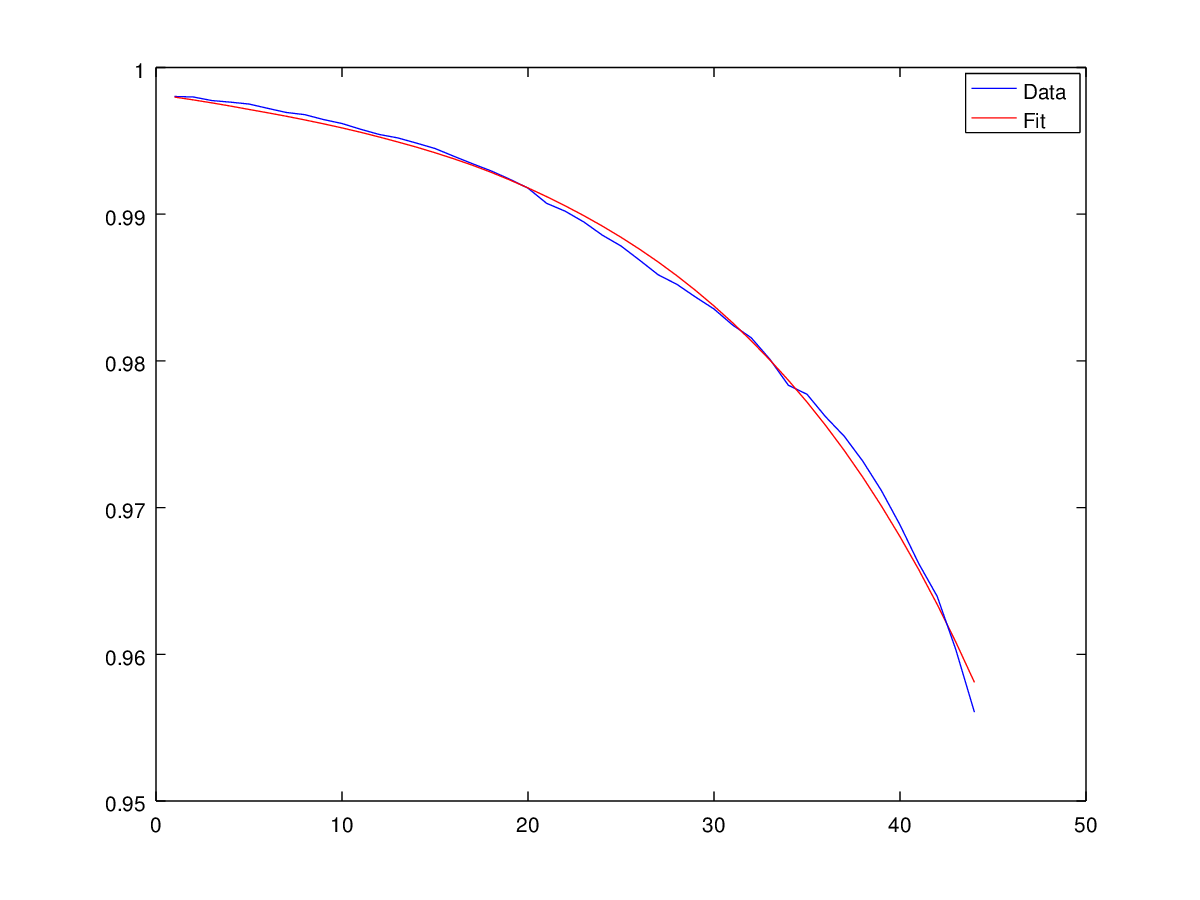
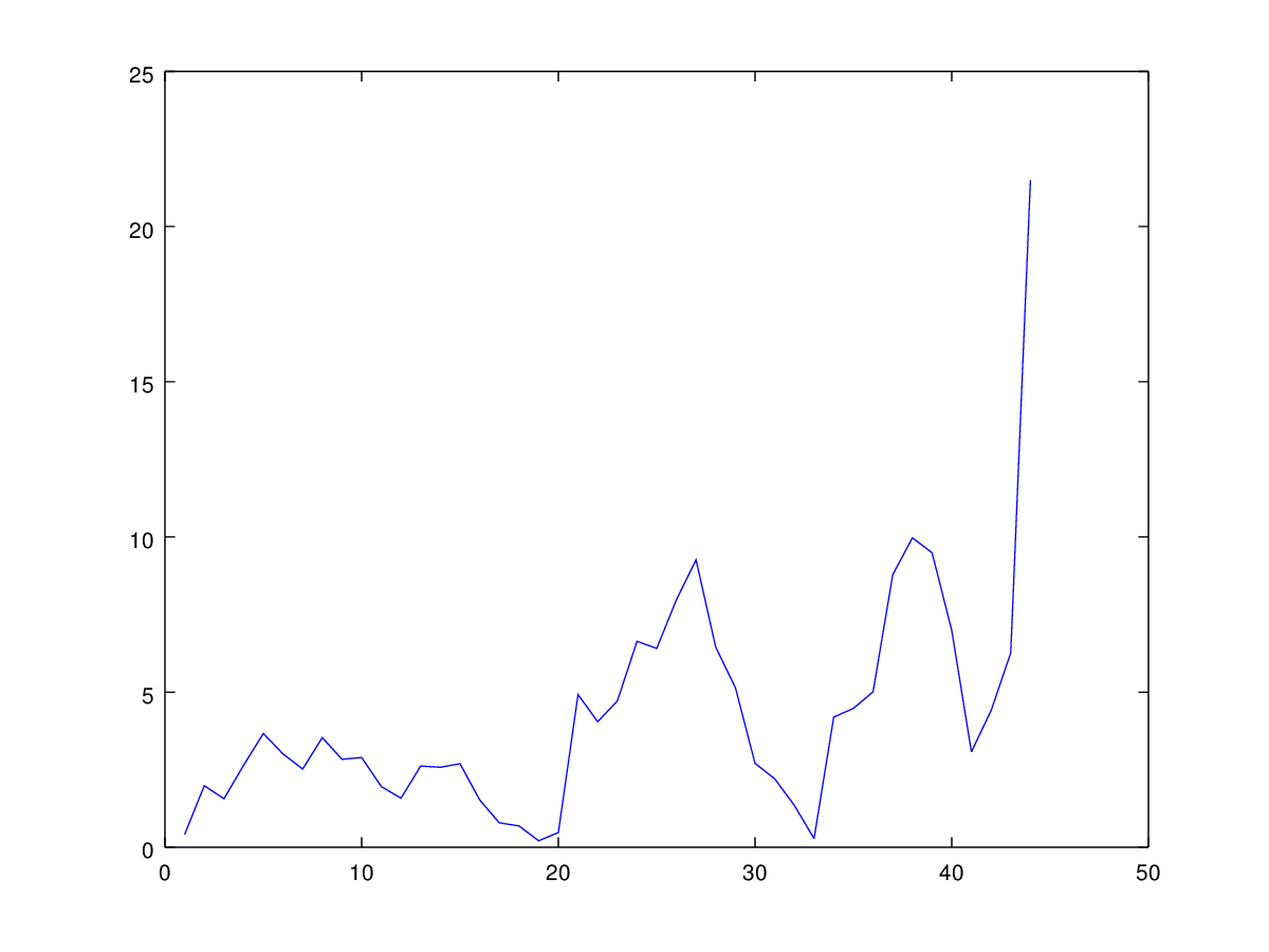
Refer to caption
(a) Longevity index data and fit
Refer to caption
(b) Pricing error generated by Kalman filter
Refer to caption
(c) Longevity index RMSE
Refer to caption
(d) State variable component Y𝑌Y
Refer to caption
(e) Mortality intensity μ𝜇\mu
Figure 2: Longevity index data and fit.

Similarly Figure 2 2(a) plots the observed longevity index data and the fit produced by (5.5) with estimated parameter sets. Figure 22(b) and 2(c), with unit in basis point, show respectively the pricing error associated to (5.5) and the root mean square pricing error (RMSE) computed over 100 Monte Carlo replications. Figure 22(d) displays time series of estimated state variable component Y𝑌Y. Figure 22(e) displays time series of estimated mortality intensity μ𝜇\mu. The simulated samples consist of 44 annual time series observations from January 1970 to January 2013.
The absence of the diffusion term in the Y𝑌Y dynamics produces rather smooth paths for Y𝑌Y and consequently for the longevity index fit. This is reasonable as longevity index data has very light oscillations along the trend, with a mean RMSE value of 15.39 bps. However, the poor data set of the longevity index, with always less than 50 annual observations for one age cohort, and the long time frame between two consecutive data can be a drawback for calibration.

6 Conclusion

We consider a polynomial diffusion state variable on compact state space to model the hybrid financial-insurance market. We include a dependence structure between OIS short rate and mortality intensity and are able to guarantee their positivity when needed. The model is parsimonious and analytically tractable. By following the benchmark approach we compute optimal premium as well as risk-minimizing strategy for life insurance liabilities. We complete our theoretical analysis by a calibration of a particular model specification to real data. As showed in Section 5, we obtain a good fitting to the MSCI and LLMA index also in the parsimonious case of a two-dimensional state variable under linear polynomial specification.

Appendix A Benchmarked risk-minimization for payment streams

We give here the general definitions and results of the benchmarked risk-minimizing method for payment streams by following mainly [6] and [4] for the presentation.

We introduce first the following Hilbert spaces

M02(,𝔾):={M:=(Mt)t[0,T]𝔾-martingale |M0=0,supt[0,T]𝔼[Mt2]<},assignsuperscriptsubscript𝑀02𝔾conditional-setassign𝑀subscriptsubscript𝑀𝑡𝑡0𝑇𝔾-martingale formulae-sequencesubscript𝑀00subscriptsupremum𝑡0𝑇𝔼delimited-[]superscriptsubscript𝑀𝑡2M_{0}^{2}({\mathbb{P}},{\mathbb{G}}):=\left.\{M:=(M_{t})_{t\in[0,T]}\ {\mathbb{G}}\text{-martingale }\right|\ M_{0}=0,\ \sup_{t\in[0,T]}\mathbb{E}\left[M_{t}^{2}\right]<\infty\},
L2(S~,,𝔾)={δl-valued 𝔾-predictable processes |𝔼[0Tδud[S~]uδu]<},superscript𝐿2~𝑆𝔾conditional-set𝛿superscript𝑙-valued 𝔾-predictable processes 𝔼delimited-[]subscriptsuperscript𝑇0subscriptsuperscript𝛿top𝑢dsubscriptdelimited-[]~𝑆𝑢subscript𝛿𝑢L^{2}(\tilde{S},{\mathbb{P}},{\mathbb{G}})=\left.\bigg{\{}\ \delta\ \ {\mathbb{R}}^{l}\text{-valued }{\mathbb{G}}\text{-predictable processes }\right|\ \mathbb{E}\left[\int^{T}_{0}\delta^{\top}_{u}\mathrm{d}[\tilde{S}]_{u}\delta_{u}\right]<\infty\bigg{\}},
(S~,,𝔾)={0TδudS~u|δL2(S~,,𝔾)},~𝑆𝔾conditional-setsubscriptsuperscript𝑇0superscriptsubscript𝛿𝑢topdifferential-dsubscript~𝑆𝑢𝛿superscript𝐿2~𝑆𝔾\mathcal{I}(\tilde{S},{\mathbb{P}},{\mathbb{G}})=\left\{\left.\int^{T}_{0}\delta_{u}^{\top}\mathrm{d}\tilde{S}_{u}\right|\delta\in L^{2}(\tilde{S},{\mathbb{P}},{\mathbb{G}})\right\},

with norms given respectively by

MM02(,𝔾):=supt[0,T]𝔼[Mt2]12=𝔼[MT2]12=supt[0,T]𝔼[[M]t]12=𝔼[[M]T]12,assignsubscriptnorm𝑀superscriptsubscript𝑀02𝔾subscriptsupremum𝑡0𝑇𝔼superscriptdelimited-[]superscriptsubscript𝑀𝑡212𝔼superscriptdelimited-[]superscriptsubscript𝑀𝑇212subscriptsupremum𝑡0𝑇𝔼superscriptdelimited-[]subscriptdelimited-[]𝑀𝑡12𝔼superscriptdelimited-[]subscriptdelimited-[]𝑀𝑇12\left\|M\right\|_{M_{0}^{2}({\mathbb{P}},{\mathbb{G}})}:=\sup_{t\in[0,T]}\mathbb{E}\left[M_{t}^{2}\right]^{\frac{1}{2}}=\mathbb{E}\left[M_{T}^{2}\right]^{\frac{1}{2}}=\sup_{t\in[0,T]}\mathbb{E}\left[[M]_{t}\right]^{\frac{1}{2}}=\mathbb{E}\left[[M]_{T}\right]^{\frac{1}{2}},
δL2(S~,,𝔾):=(𝔼[0Tδud[S~]uδu])12,assignsubscriptnorm𝛿superscript𝐿2~𝑆𝔾superscript𝔼delimited-[]subscriptsuperscript𝑇0subscriptsuperscript𝛿top𝑢dsubscriptdelimited-[]~𝑆𝑢subscript𝛿𝑢12\left\|\delta\right\|_{L^{2}(\tilde{S},{\mathbb{P}},{\mathbb{G}})}:=\left(\mathbb{E}\left[\int^{T}_{0}\delta^{\top}_{u}\mathrm{d}[\tilde{S}]_{u}\delta_{u}\right]\right)^{\frac{1}{2}},
0TδudS~u(S~,,𝔾):=𝔼[(0TδudS~u)2]12,assignsubscriptnormsubscriptsuperscript𝑇0superscriptsubscript𝛿𝑢topdifferential-dsubscript~𝑆𝑢~𝑆𝔾𝔼superscriptdelimited-[]superscriptsubscriptsuperscript𝑇0superscriptsubscript𝛿𝑢topdifferential-dsubscript~𝑆𝑢212\left\|\int^{T}_{0}\delta_{u}^{\top}\mathrm{d}\tilde{S}_{u}\right\|_{\mathcal{I}(\tilde{S},{\mathbb{P}},{\mathbb{G}})}:=\mathbb{E}\left[\left(\int^{T}_{0}\delta_{u}^{\top}\mathrm{d}\tilde{S}_{u}\right)^{2}\right]^{\frac{1}{2}},

for MM02(,𝔾)𝑀superscriptsubscript𝑀02𝔾M\in M_{0}^{2}({\mathbb{P}},{\mathbb{G}}) and δL2(S~,,𝔾)𝛿superscript𝐿2~𝑆𝔾\delta\in L^{2}(\tilde{S},{\mathbb{P}},{\mathbb{G}}). Lemma 3.4 of [4] (or Lemma 2.1 of [45]) shows that (S~,,𝔾)~𝑆𝔾\mathcal{I}(\tilde{S},{\mathbb{P}},{\mathbb{G}}) is a stable subspace of M02(,𝔾)superscriptsubscript𝑀02𝔾M_{0}^{2}({\mathbb{P}},{\mathbb{G}}). In particular, for every δL2(S~,,𝔾)𝛿superscript𝐿2~𝑆𝔾\delta\in L^{2}(\tilde{S},{\mathbb{P}},{\mathbb{G}}) we have

δL2(S~,,𝔾)=0TδudS~u(S~,,𝔾)=0TδudS~uM02(,𝔾).subscriptnorm𝛿superscript𝐿2~𝑆𝔾subscriptnormsubscriptsuperscript𝑇0superscriptsubscript𝛿𝑢topdifferential-dsubscript~𝑆𝑢~𝑆𝔾subscriptnormsubscriptsuperscript𝑇0superscriptsubscript𝛿𝑢topdifferential-dsubscript~𝑆𝑢superscriptsubscript𝑀02𝔾\left\|\delta\right\|_{L^{2}(\tilde{S},{\mathbb{P}},{\mathbb{G}})}=\left\|\int^{T}_{0}\delta_{u}^{\top}\mathrm{d}\tilde{S}_{u}\right\|_{\mathcal{I}(\tilde{S},{\mathbb{P}},{\mathbb{G}})}=\left\|\int^{T}_{0}\delta_{u}^{\top}\mathrm{d}\tilde{S}_{u}\right\|_{M_{0}^{2}({\mathbb{P}},{\mathbb{G}})}.
Definition A.1.

An L2superscript𝐿2L^{2}-admissible strategy is a process δ:=(δt)t[0,T]assign𝛿subscriptsubscript𝛿𝑡𝑡0𝑇\delta:=(\delta_{t})_{t\in[0,T]} such that

  • (1)

    δL2(S~,,𝔾)𝛿superscript𝐿2~𝑆𝔾\delta\in L^{2}(\tilde{S},{\mathbb{P}},{\mathbb{G}}),

  • (2)

    the associated benchmarked value process S~δsuperscript~𝑆𝛿\tilde{S}^{\delta} with

    S~tδ:=δtS~t,t[0,T]formulae-sequenceassignsubscriptsuperscript~𝑆𝛿limit-from𝑡superscriptsubscript𝛿𝑡topsubscript~𝑆𝑡𝑡0𝑇\tilde{S}^{\delta}_{t-}:=\delta_{t}^{\top}\tilde{S}_{t},\ \ \ \ t\in[0,T]

    is in M02(,𝔾)superscriptsubscript𝑀02𝔾M_{0}^{2}({\mathbb{P}},{\mathbb{G}}).

Now we fix a process A𝐴A as defined in (3.4) which models the benchmarked cumulative payments towards a policyholder.

Definition A.2.

The benchmarked cumulative cost process Cδ:=(Ctδ)t[0,T]assignsuperscript𝐶𝛿subscriptsuperscriptsubscript𝐶𝑡𝛿𝑡0𝑇C^{\delta}:=(C_{t}^{\delta})_{t\in[0,T]} of a L2superscript𝐿2L^{2}-admissible strategy δ𝛿\delta associated to A𝐴A is defined by

Ctδ=S~tδ0tδudS~u+At,t[0,T].formulae-sequencesuperscriptsubscript𝐶𝑡𝛿subscriptsuperscript~𝑆𝛿𝑡superscriptsubscript0𝑡subscript𝛿𝑢differential-dsubscript~𝑆𝑢subscript𝐴𝑡𝑡0𝑇C_{t}^{\delta}=\tilde{S}^{\delta}_{t}-\int_{0}^{t}\delta_{u}\mathrm{d}\tilde{S}_{u}+A_{t},\ \ \ \ t\in[0,T].
Definition A.3.

The risk process Rδ:=(Rtδ)t[0,T]assignsuperscript𝑅𝛿subscriptsubscriptsuperscript𝑅𝛿𝑡𝑡0𝑇R^{\delta}:=(R^{\delta}_{t})_{t\in[0,T]} of an L2superscript𝐿2L^{2}-admissible strategy δ𝛿\delta is defined by

Rtδ=𝔼[(CTδCtδ)2|𝒢t],t[0,T].formulae-sequencesuperscriptsubscript𝑅𝑡𝛿𝔼delimited-[]conditionalsuperscriptsuperscriptsubscript𝐶𝑇𝛿superscriptsubscript𝐶𝑡𝛿2subscript𝒢𝑡𝑡0𝑇R_{t}^{\delta}=\mathbb{E}\left.\left[(C_{T}^{\delta}-C_{t}^{\delta})^{2}\right|{\mathcal{G}}_{t}\right],\ \ \ \ t\in[0,T].
Definition A.4.

An L2superscript𝐿2L^{2}-admissible strategy δ¯¯𝛿\bar{\delta} is called benchmarked risk-minimizing for A𝐴A if

  • (1)

    S~Tδ¯=0superscriptsubscript~𝑆𝑇¯𝛿0\tilde{S}_{T}^{\bar{\delta}}=0 {\mathbb{P}}-a.s.,

  • (2)

    Rtδ¯Rtδsuperscriptsubscript𝑅𝑡¯𝛿superscriptsubscript𝑅𝑡𝛿R_{t}^{\bar{\delta}}\leqslant R_{t}^{\delta} {\mathbb{P}}-a.s. for every t[0,T]𝑡0𝑇t\in[0,T] and for any L2superscript𝐿2L^{2}-admissible strategy δ𝛿\delta such that S~Tδ¯=S~Tδsuperscriptsubscript~𝑆𝑇¯𝛿superscriptsubscript~𝑆𝑇𝛿\tilde{S}_{T}^{\bar{\delta}}=\tilde{S}_{T}^{\delta} {\mathbb{P}}-a.s., δ¯u=δusubscript¯𝛿𝑢subscript𝛿𝑢\bar{\delta}_{u}=\delta_{u} {\mathbb{P}}-a.s. for all ut𝑢𝑡u\leqslant t.

Lemma A.5.

The benchmarked cumulative cost process of any benchmarked risk-minimizing strategy is a (,𝔾)𝔾({\mathbb{P}},{\mathbb{G}})-martingale.

Proof.

This lemma is a combination of Lemma 3.5 of [6] and Lemma A.4 of [37]. ∎

Lemma A.6.

The benchmarked value process associated to a benchmarked risk-minimizing strategy δ¯¯𝛿\bar{\delta} for A𝐴A is given by

S~tδ¯=𝔼[ATAt|𝒢t],t[0,T].formulae-sequencesuperscriptsubscript~𝑆𝑡¯𝛿𝔼delimited-[]subscript𝐴𝑇conditionalsubscript𝐴𝑡subscript𝒢𝑡𝑡0𝑇\tilde{S}_{t}^{\bar{\delta}}=\mathbb{E}\left.\left[A_{T}-A_{t}\right|{\mathcal{G}}_{t}\right],\ \ \ \ t\in[0,T].
Proof.

The proof is a straightforward consequence of Lemma A.5 and Lemma 3.12 of [37]. ∎

The following theorem gives the solution of the benchmarked risk-minimizing problem.

Theorem A.7.

Let

AT=𝔼[AT]+0T(δuA)dS~u+LTA,a.s.,subscript𝐴𝑇𝔼delimited-[]subscript𝐴𝑇superscriptsubscript0𝑇superscriptsubscriptsuperscript𝛿𝐴𝑢topdifferential-dsubscript~𝑆𝑢subscriptsuperscript𝐿𝐴𝑇a.s.A_{T}=\mathbb{E}[A_{T}]+\int_{0}^{T}\left(\delta^{A}_{u}\right)^{\top}\mathrm{d}\tilde{S}_{u}+L^{A}_{T},\ \ \ \ {\mathbb{P}}-\text{a.s.}, (A.1)

be the Galtchouk-Kunita-Watanabe decomposition141414See [1] for an overview of Galtchouk-Kunita-Watanabe decomposition. of ATsubscript𝐴𝑇A_{T}, where 0TδuAdS~usuperscriptsubscript0𝑇subscriptsuperscript𝛿𝐴𝑢differential-dsubscript~𝑆𝑢\int_{0}^{T}\delta^{A}_{u}\mathrm{d}\tilde{S}_{u} is the projection of (AT𝔼[AT])subscript𝐴𝑇𝔼delimited-[]subscript𝐴𝑇\left(A_{T}-\mathbb{E}[A_{T}]\right) on the space (S~,,𝔾)~𝑆𝔾\mathcal{I}(\tilde{S},{\mathbb{P}},{\mathbb{G}}) with δAL2(S~,,𝔾)superscript𝛿𝐴superscript𝐿2~𝑆𝔾\delta^{A}\in L^{2}(\tilde{S},{\mathbb{P}},{\mathbb{G}}) and LAM02(,𝔾)superscript𝐿𝐴superscriptsubscript𝑀02𝔾L^{A}\in M_{0}^{2}({\mathbb{P}},{\mathbb{G}}) is {\mathbb{P}}-strongly orthogonal to (S~,,𝔾)~𝑆𝔾\mathcal{I}(\tilde{S},{\mathbb{P}},{\mathbb{G}}). The unique benchmarked risk-minimizing strategy δ¯¯𝛿\bar{\delta} for A𝐴A is given by δ¯=δA¯𝛿superscript𝛿𝐴\bar{\delta}=\delta^{A}. The associated benchmarked cumulative cost process is

Ctδ¯=𝔼[AT]+LtA=C0δ¯+LtA,t[0,T],formulae-sequencesuperscriptsubscript𝐶𝑡¯𝛿𝔼delimited-[]subscript𝐴𝑇subscriptsuperscript𝐿𝐴𝑡superscriptsubscript𝐶0¯𝛿subscriptsuperscript𝐿𝐴𝑡𝑡0𝑇C_{t}^{\bar{\delta}}=\mathbb{E}\left[A_{T}\right]+L^{A}_{t}=C_{0}^{\bar{\delta}}+L^{A}_{t},\ \ \ \ t\in[0,T],

and the benchmarked value process is

S~tδ¯=𝔼[ATAt|𝒢t],t[0,T].formulae-sequencesuperscriptsubscript~𝑆𝑡¯𝛿𝔼delimited-[]subscript𝐴𝑇conditionalsubscript𝐴𝑡subscript𝒢𝑡𝑡0𝑇\tilde{S}_{t}^{\bar{\delta}}=\mathbb{E}\left.\left[A_{T}-A_{t}\right|{\mathcal{G}}_{t}\right],\ \ \ \ t\in[0,T].
Proof.

The theorem follows from Lemma A.5 and Theorem 2.1 of [37]. ∎

As the classic risk-minimizing strategy, the crucial point of the solution of the benchmarked risk-minimizing strategy is finding the Galtchouk-Kunita-Watanabe decomposition (A.1).

We stress that, the orthogonal projection provided by the decomposition (A.1) shows that every benchmarked cumulative payment ATsubscript𝐴𝑇A_{T} has a perfectly hedgeable part 0T(δuA)dS~usuperscriptsubscript0𝑇superscriptsubscriptsuperscript𝛿𝐴𝑢topdifferential-dsubscript~𝑆𝑢\int_{0}^{T}\left(\delta^{A}_{u}\right)^{\top}\mathrm{d}\tilde{S}_{u} and a totally unhedgeable part (𝔼[AT]+LTA)𝔼delimited-[]subscript𝐴𝑇subscriptsuperscript𝐿𝐴𝑇\left(\mathbb{E}\left[A_{T}\right]+L^{A}_{T}\right) covered by the benchmarked cumulative cost process C𝐶C. Furthermore, according to Lemma A.6, the benchmarked value process associated to the unique benchmarked risk-minimizing strategy δ¯¯𝛿\bar{\delta} for a given benchmarked cumulative payment process A𝐴A coincides with the benchmarked value of the real world pricing formula given in (3.5), i.e.

S~tδ¯=VtSt,t[0,T].formulae-sequencesuperscriptsubscript~𝑆𝑡¯𝛿subscript𝑉𝑡subscriptsuperscript𝑆𝑡𝑡0𝑇\tilde{S}_{t}^{\bar{\delta}}=\frac{V_{t}}{S^{*}_{t}},\ \ \ \ t\in[0,T].

The benchmarked hedging problem and its relation with the real world pricing formula have already been studied in [5] and [6] in the case of a T𝑇T-claims D¯¯𝐷\bar{D}, i.e. when the dividend process D𝐷D is given by

Dt=𝟏{t=T}D¯,t[0,T],formulae-sequencesubscript𝐷𝑡subscript1𝑡𝑇¯𝐷𝑡0𝑇D_{t}=\mathbf{1}_{\left\{t=T\right\}}\bar{D},\ \ \ \ t\in[0,T],

with D¯¯𝐷\bar{D} a square integrable 𝒢𝒢{\mathcal{G}}-measurable random variable. The real world pricing formula is reduced to

Vt=St𝔼[D¯ST|𝒢t],t[0,T[,V_{t}=S_{t}^{*}\mathbb{E}\left.\left[\frac{\bar{D}}{S^{*}_{T}}\right|{\mathcal{G}}_{t}\right],\ \ \ \ t\in[0,T[,

which is the original definition of fair price given in e.g. [42] for a T𝑇T-claim D¯¯𝐷\bar{D}. In this case, if the T𝑇T-claim admits a self-financing strategy, then thanks to the supermartingale property of the benchmark portfolio in Definition (3.4), V𝑉V corresponds to the least expensive self-financing portfolio which replicates D¯¯𝐷\bar{D}.

References

  • [1] J. P. Ansel and C. Stricker. Décomposition de Kunita-Watanabe. Séminaire de Probabilités de Strasbourg, 27:30–32, 1993.
  • [2] A. Antonov and M. Spector. Analytical approximations for short rate models, 2010. Available at SSRN: http://ssrn.com/abstract=1692624 or http://dx.doi.org/10.2139/ssrn.1692624.
  • [3] K. Back, T.R. Bielecki, C. Hipp, S. Peng, and W. Schachermayer. Stochastic Methods in Finance. Lectures given at the C.I.M.E.-E.M.S. summer school held in Bressanone/Brixen, Italy, July 6-12, 2003. Springer, 2004.
  • [4] J. Barbarin. Risk-minimizing strategies for life insurance contracts with surrender option, 2007. Available at SSRN: http://ssrn.com/abstract=1334580 or http://dx.doi.org/10.2139/ssrn.1334580.
  • [5] F. Biagini. Evaluating hybrid products: the interplay between financial and insurance markets. In R. Dalang, M. Dozzi, and F. Russo, editors, Stochastic Analysis, Random Fields and Applications VII, Progress in Probability 67. Birkhäuser Verlag, 2013.
  • [6] F. Biagini, A. Cretarola, and E. Platen. Local risk-minimization under the benchmark approach. Mathematics and Financial Economics, 8(2):109–134, 2014.
  • [7] F. Biagini and M. Pratelli. Local risk minimization and numéraire. Journal of Applied Probability, 36(4):1126–1139, 1999.
  • [8] F. Biagini, T. Rheinländer, and I. Schreiber. Risk-minimization for life insurance liabilities with basis risk. Mathematics and Financial Economics, 10(2):151–178, 2016.
  • [9] F. Biagini and I. Schreiber. Risk-minimization for life insurance liabilities. SIAM Journal on Financial Mathematics, 4:243–264, 2013.
  • [10] T. R. Bielecki and M. Rutkowski. Credit Risk: Modelling, Valuation and Hedging. Springer-Finance, Springer, second edition, 2004.
  • [11] D. Blake, A. J. G. Cairns, and K. Dowd. Living with mortality: Longevity bonds and other mortality-linked securities. British Actuarial Journal, 12:153––228, 2008.
  • [12] A. J. G. Cairns, D. Blake, and K. Dowd. Pricing death: frameworks for valuation and securitization of mortality risk. ASTIN Bulletin, 36(1):79–120, 2006.
  • [13] M. Dacorogna and M. Cadena. Exploring the dependence between mortality and market risks. SCOR Papers, 2015.
  • [14] M. Dahl and T. Møller. Valuation and hedging of life insurance liabilities with systematic mortality risk. Insurance: Mathematics and Economics, 39(2):193––217, 2006.
  • [15] G. Deelstra, M. Grasselli, and C. Van Weverberg. The role of the dependence between mortality and interest rates when pricing guaranteed annuity options, 2015. Available at SSRN: http://ssrn.com/abstract=2667939 or http://dx.doi.org/10.2139/ssrn.2667939.
  • [16] F. Delbaen and W. Schachermayer. A general version of the fundamental theorem of asset pricing. Mathemathische Annalen, 300(1):463–520, 1994.
  • [17] F. Delbaen and H. Shirakawa. An interest rate model with upper and lower bounds. Asia-Pacific Financial Markets, 9(3):191–209, 2002.
  • [18] C. Dellacherie and P.A. Meyer. Probabilities and Potential B: Theory of Martingales. Amsterdam: North Holland, 1982.
  • [19] L. Demetrius. Mortality plateaus and directionality theory. Proceedings of the Royal Society B: Biological Sciences, 268(1480):2029–37, 2001.
  • [20] K. Du and E. Platen. Three-benchmarked risk minimization for jump diffusion markets. Quantitative Finance Research Centre, Research Paper No. 296, 2011. Available at SSRN: http://ssrn.com/abstract=2170169 or http://dx.doi.org/10.2139/ssrn.2170169.
  • [21] J. C. Duan and J. G. Simonato. Estimating and testing exponential-affine term structure models by Kalman filter. Review of Quantitative Finance and Accounting, 13(2):111–135, 1999.
  • [22] R. Durrett. Stochastic Calculus: A Practical Introduction. Probability and Stochastics Series. CRC Press, Boca Raton, FL, 1996.
  • [23] D. Filipović and M. Larsson. Polynomial diffusions and applications in finance. Finance and Stochastics, 2016. Forthcoming.
  • [24] D. Filipović, M. Larsson, and A. B. Trolle. Linear-rational term structure models. Journal of Finance, 2016. Forthcoming; Swiss Finance Institute Research Paper, 14-15.
  • [25] B. Flesaker and L.P. Hughston. Positive interest. Risk, 9(1):46–49, 1996.
  • [26] H. Föllmer and D. Sondermann. Hedging of non-redundant contingent claims. In W. Hildenbrand and A. Mas-Colell, editors, Contributions to Mathematical Economics, pages 205–223. North Holland, 1986.
  • [27] A. C. Harvey. Forecasting, Structural Models and the Kalman Filter. Cambridge University Press, New York, 1989.
  • [28] H. Hulley and M. Schweizer. M6superscript𝑀6M^{6}-on minimal market models and minimal martingale measures. In C. Chiarella and A. Novikov, editors, Contemporary Quantitative Finance. Essays in Honour of Eckhard Platen, pages 35–51. Springer, 2010.
  • [29] J. Jacod. Calcul Stochastique et Problèmes de Martingales. Springer-Verlag, 1979.
  • [30] F. Jamshidian. Valuation of credit default swaps and swaptions. Finance and Stochastics, 8(3):343–371, 2004.
  • [31] S. F. Jarner and E. M. Kryger. Modelling adult mortality in small populations: the Saint model. ASTIN Bulletin, 41(02):377–418, 2011.
  • [32] M. Larsson and S. Pulido. Polynomial preserving diffusions on compact quadric sets, 2015. Available at http://arxiv.org/abs/1511.03554.
  • [33] J. Li and A. Szimayer. The uncertain mortality intensity framework: pricing and hedging unit-linked life insurance contracts. Insurance: Mathematics and Economics, 49:471–486, 2011.
  • [34] N. Lima and N. Privault. Analytic bond pricing for short rate dynamics evolving on matrix Lie groups. Quantitative Finance, 16(1), 2016.
  • [35] X. Liu, R. Mamon, and H. Gao. A comonotonicity-based valuation method for guaranteed annuity options. J. Computational Applied Mathematics, 250:58–69, 2013.
  • [36] J. Lund and F. Alle. Non-linear Kalman filtering techniques for term-structure models. Working paper, Aarhus School of Business, 1997.
  • [37] T. Møller. Risk-minimizing hedging strategies for insurance payment processes. Finance and Stochastics, 5:419–446, 1998.
  • [38] T. Møller. Risk-minimizing hedging strategies for unit-linked life insurance contracts. ASTIN Bulletin, 28(1):17–47, 1998.
  • [39] E. Platen. A benchmark framework for risk management. In Stochastic Processes and Applications to Mathematical Finance, pages 305–335. World Scientific, 2004.
  • [40] E. Platen. Diversified portfolios with jumps in a benchmark framework. Asia-Pacific Financial Markets, 11(1):1–22, 2004.
  • [41] E. Platen. A benchmark approach to finance. Mathematical Finance, 16(1):131––151, 2006.
  • [42] E. Platen and D. Heath. A Benchmark Approach to Quantitative Finance. Springer, Berlin, 2006.
  • [43] L. C. G. Rogers and D. Williams. Diffusions, Markov Processes and Martingales. Cambridge University Press, 1994.
  • [44] E. Schlogl and D. Sommer. On short rate processes and their implications for term structure movements, 1994. Available at SSRN: http://ssrn.com/abstract=5768.
  • [45] M. Schweizer. A guided tour through quadratic hedging approaches. In Option Pricing, Interest Rates and Risk Management, pages 538–574. Cambridge University Press, Cambridge, UK, 2001.