Is the motion of a single SPH particle droplet/solid physically correct?

Abstract

In recent years the Smoothed Particle Hydrodynamics (SPH) approach gained popularity in modeling multiphase and free-surface flows. In many situations, due to certain reasons, interface and free-surface fragmentation occurs. As a result single SPH particle solids/droplets of one phase can appear and travel through other phases. In this paper we investigate this issue focusing on a movement of such single SPH particles. The main questions we try to answer here are: is movement of such particles physically correct? What is its physical size? How numerical parameters affect on it? With this in mind we performed simple simulations of solid particles falling due to gravity in a fluid. Considering three different diameters of a single particle, we compared values of the drag coefficient and the velocity obtained through the SPH approach with the experimental and the analytical reference data. In the way to accurately model multiphase flows with free-surfaces we proposed and validated a novel SPH formulation.

1 Introduction

The Smoothed Particle Hydrodynamics method (SPH) is a mesh-free, particle-based approach for fluid-flow modelling. In the early stage it was developed to simulate some astrophysical phenomena at the hydrodynamic level [1]. The main idea behind the SPH method is to introduce kernel interpolants for flow quantities in order to represent fluid dynamics by a set of particle evolution equations. Due to its Lagrangian nature, for multiphase flows, there is no necessity to handle (reconstruct or track) the interface shape as in the grid-based methods. Therefore, there is no additional numerical diffusion related to the interface handling. For this reason and the fact that the SPH approach is well suited to problems with large density contrast, free-surfaces and complex geometries, the SPH method is increasingly used for hydro-engineering and geophysical applications, for review see [2, 3].

In many situations, due to both: physical processes and numerical errors, the interface in multi-phase flows and the surface in free-surface flows can be fragmented, see [2, 4, 5, 6, 7]. As a result, the single SPH particle solids/droplets (or even bubbles) can appear and move in the opposite phase or travel without any friction through the regions without particles (representing gaseous phase in free-surface flows). Since the reason of the appearance of single SPH particle solids/droplets may be different depending on the nature and scale of the problem, we do not intent to discuss the causes in detail. However, in some papers, eg. [8, 9], the authors model a dispersed phase (droplets) moving in the other liquid as a single or a small number of the SPH particles. In the present paper, we focus on the problem of physical correctness of such single particle solids/droplets motion. We try to answer the following questions: is the motion of a single particle droplet physically correct? What is such a droplet’s diameter? What is an influence of the SPH numerical parameters such as $h$, $h/\Delta r$ or the shape of the kernel on the motion of the single particle?

In the following considerations we assume that the reader is familiar with the SPH basics. Those not familiar with the method may find useful information on the SPHERIC - SPH European Research Interest Community web page [10]. Another reliable source of information is a handbook by Violeau (2012) [3].

2 Multiphase SPH formulation

The full set of governing equations for incompressible viscous flows is composed of the Navier-Stokes (N-S) equation

$$\frac{d\mathbf{u}}{dt}=-\frac{1}{\varrho}\nabla p+\frac{1}{\varrho}\left(\nabla\mu\cdot\nabla\right)\mathbf{u}+\mathbf{f},$$ (1)

where $\varrho$ is the density, $\mathbf{u}$ velocity, $t$ time, $p$ pressure, $\mu$ the dynamic viscosity and $\mathbf{f}$ an acceleration; the continuity equation

$$\frac{d\varrho}{dt}=-\varrho\nabla\cdot\mathbf{u}\xrightarrow{\varrho=const}\nabla\cdot\mathbf{u}=0,$$ (2)

and the advection equation (Lagrangian formalism)

$$\frac{d\mathbf{r}}{dt}=\mathbf{u},$$ (3)

where $\mathbf{r}$ denotes position of fluid element.

The governing equations can be expressed in the SPH formalism in many different ways. In general, two SPH approximations: integral interpolation and discretization, lead to the the basic SPH relationship

$$\left\langle A\right\rangle(\mathbf{r})=\sum_{b}A(\mathbf{r}_{b})W(\mathbf{r}-\mathbf{r}_{b},h)\Omega_{b},$$ (4)

where $A$ is a physical field (in a sake of simplicity we consider a scalar field only), $W$ is a weighting function (kernel) with parameter $h$ called the smoothing length, while $\Omega$ is the volume of the SPH particle. In the present paper we use the Wendland kernel [11] in the form

$$W(\mathbf{r},h)=C\left\{\begin{array}[]{cl}\left(1-q/2\right)^{4}(2q+1)&\text{for}\;\;q\leq 2,\\ 0&\text{otherwise},\\ \end{array}\right.$$ (5)

where $q=|\mathbf{r}|/h$ and the normalization constant is $C=7/4\pi h^{2}$ (in 2D) or $21/16\pi h^{3}$ (in 3D). For details how the choice of the kernel and smoothing length affect results see [12]. It is important to note here that the SPH basic approximation, Eq. (4), is common also in other numerical particles-based approaches, e.g. Moving Particle Semi-implicit Method (MPS) [13]. The SPH method differs from other methods in aspect of approximation of differentiation operator. Assuming the kernel symmetry, nabla operator can be shifted from the action on the physical field to the kernel

$$\left\langle\nabla A\right\rangle(\mathbf{r})=\sum_{b}A(\mathbf{r}_{b})\nabla W(\mathbf{r}-\mathbf{r}_{b},h)\Omega_{b}.$$ (6)

It is important to note that although different SPH formulations can be obtained from the same governing equations, some of them may not by applicable for certain types of flows. For instance, the most common SPH form of the N-S pressure term

$$\left\langle\frac{\nabla p}{\varrho}\right\rangle_{a}=-\sum_{b}m_{b}\left(\frac{p_{a}}{\varrho_{a}^{2}}+\frac{p_{b}}{\varrho_{b}^{2}}\right)\nabla_{a}W_{ab},$$ (7)

where $\nabla_{a}W_{ab}=\nabla_{a}W(\mathbf{r}_{a}-\mathbf{r}_{b},h)$, is very useful for modelling single-phase flows with free-surfaces. However, when applied for multi-phase flows with interfaces it leads to some instabilities at interface, for details see [4, 14]. To the best of our knowledge, there are three SPH formulations constructed to model multi-phase flows: Colagrossi and Landrini (2003) [4], Hu and Adams (2006) [15] and Grenier et al. (2009) [5]. For the purposes of this work, we decided to use the Hu and Adams (2006) formalism. In this approach, the N-S pressure term becomes

$$\left\langle\frac{\nabla p}{\varrho}\right\rangle_{a}=-\frac{1}{m_{a}}\sum_{b}\left(\frac{p_{a}}{\Theta_{a}^{2}}+\frac{p_{b}}{\Theta_{b}^{2}}\right)\nabla_{a}W_{ab},$$ (8)

where $\Theta$ is inverse of particle volume, and the viscous N-S term is

$$\left\langle\left(\nabla\mu\cdot\nabla\right)\mathbf{u}\right\rangle_{a}=\frac{1}{m_{a}}\sum_{b}\frac{2\mu_{a}\mu_{b}}{\mu_{a}+\mu_{b}}\left(\frac{1}{\Theta_{a}^{2}}+\frac{1}{\Theta_{b}^{2}}\right)\frac{\mathbf{r}_{ab}\cdot\nabla_{a}W_{ab}}{r_{ab}^{2}+\eta^{2}}\mathbf{u}_{ab},$$ (9)

where $\eta=0.01h$ is a small regularizing parameter, while the continuity equation has the form (of the density definition)

$$\varrho_{a}=m_{a}\sum_{b}W_{ab}=m_{a}\Theta_{a}.$$ (10)

In this variant of the continuity equation the density field is represented only by a spatial distribution of neighbouring particles, but not by their masses. Therefore, in multi-phase flows, particles located near an interface but belonging to different phases may interact without having their density affected by the other fluid. The main drawback of Eq. (10) is inability to deal with free-surfaces. Lack of the SPH particles apart from the fluid causes the underestimation of the density field near the free-surfaces. To overcome this problem, we decided to take a variation of Eq. (10) (assuming constant mass of particles)

$$\delta\varrho_{a}=m_{a}\sum_{b}\left(\delta\mathbf{r}_{a}-\delta\mathbf{r}_{b}\right)\cdot\nabla_{a}W_{ab}.$$ (11)

The new variant of the continuity equation can be explicitly obtained from Eq. (11) by differentiation with respect to time

$$\frac{d\varrho_{a}}{dt}=m_{a}\sum_{b}\mathbf{u}_{ab}\cdot\nabla_{a}W_{ab}.$$ (12)

It is important to note that Eqs. (12) and (8) are variationally consistent, for details see [5, 16]. The definite advantage in using Eq. (12) over (10) is that the density only varies when particles move relative to each other. Therefore, despite a decrease of number of particles near the free-surface, this does not affect significantly the calculation of the density field (except the accuracy – smaller number of particles within the kernel range). The important difference between the Hu and Adams (2006) formulation and our approach is that we do not calculate $\Theta_{a}$ by summation over neighbouring particles, cf. Eq. (10). Instead, in Eqs. (8) and (9), we explicitly write $\Theta_{a}=\varrho_{a}/m_{a}$.

In the present work, we decided to use the most common method of implementing the incompresibility – Weakly Compressible SPH (WCSPH). It involves the set of governing equations closed by a suitably-chosen, artificial equation of state, $p=p(\varrho)$. Following the mainstream, we decided to use the Tait equation of state

$$p=\frac{c^{2}\varrho_{0}}{\gamma}\left[\left(\frac{\varrho}{\varrho_{0}}\right)^{\gamma}-1\right],$$ (13)

where $\varrho_{0}$ is the initial density. The sound speed $c$ and a parameter $\gamma$ are suitably chosen to reduce the density fluctuations down to $1\%$. In the present work we set $\gamma=7$ and $c$ at the level at least 10 times higher than the maximal fluid velocity. It is worth noting that two alternative incompressibility treatments exists: Incompressible SPH (ISPH) where the incompressibility constaint is explicity enforced through the pressure correction procedure to satisfy $\nabla\cdot\mathbf{u}=0$ [12, 17, 18, 19, 20] and Godunov SPH (GSPH) where the acoustic Riemann solver is used [21]. The boundary conditions are fulfilled applying the ghost-particle method [12, 17].

In order to validate the proposed formulation, we decided to model the Rayleigh-Taylor instability, which is one of the generic multi-phase tests. Our case involves two immiscible fluids enclosed in a rectangular domain of the edges’ sizes: $L_{x}=L$ and $L_{y}=2L$. Initially, the phases are separated by the interface located at $y/L-1-0.15\sin{(2\pi x/L)}$. The density and viscosity ratios between the upper (U) and the lower (L) phases are: $\varrho_{U}/\varrho_{L}=1.8$ and $\nu_{U}/\nu_{L}=1$ respectively. Since the system is subject to gravity, $g$, and there is no surface tension, the system destabilizes resulting in generation of vorticity. The Reynolds number of the considered case is $Re=g^{1/2}L^{3/2}\nu_{L}^{-1}=420$.

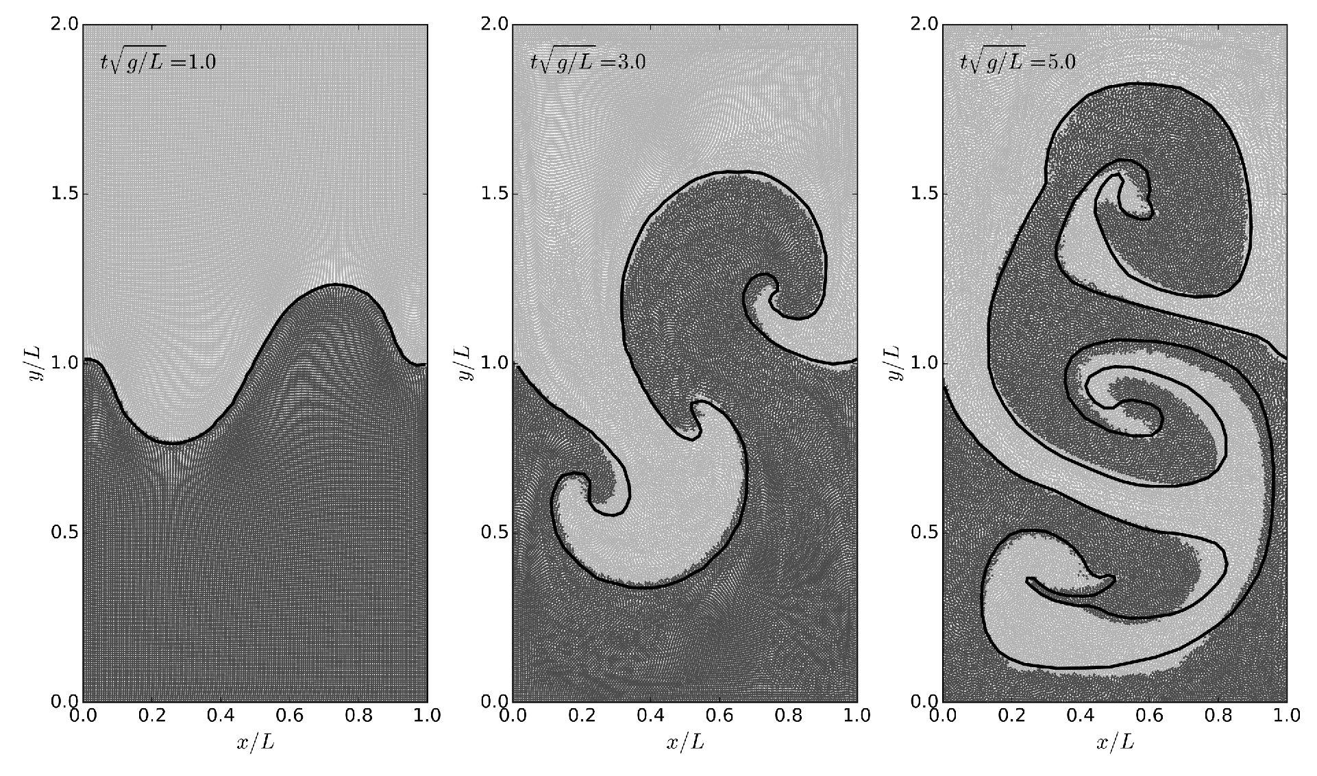
Figure 1: The Rayleigh-Taylor instability ($Re=420$) calculated using the proposed SPH formalism ($h/L=1/64$, $h/\Delta r=2.5$); black line denotes the interface position calculated using the Level-Set method ($312\times 624$ cells) by Grenier et al. (2009) [5].

The simulations were performed for $h/L=1/64$, $h/\Delta r=2.5$ and the Wendland kernel. Figure 1 presents particle positions at $t(g/L)^{1/2}=1$, $3$ and $5$ compared with the reference solutions from the Level-Set method ($312\times 624$ cells) computed by Grenier et al. (2009) [5] (black line). The results obtained with SPH show good agreement with the reference data.

3 Single particle droplets/solids

To illustrate interface fragmentation problem, we consider the multi-phase dam-breaking problem whose evolution is presented in Fig. 2. This simulation involves two liquid columns: black ($B$) and gray ($G$) enclosed in the square box of the edge size $2H$, where $H$ is the heigh of the black column. The density and viscosity ratios between phases are respectively $\varrho_{B}/\varrho_{G}=4$ and $\mu_{B}/\mu_{G}=2$. The Reynolds number is $Re=\varrho_{B}g^{1/2}H^{3/2}\mu_{B}^{-1}=2000$. The simulations were performed for $h/H=1/32$, $h/\Delta r=2$ and the Wendland kernel. Due to the gravity, $g$, the denser (black) fluid spreads over the bottom of the tank. Since the tongue of black phase propagates, it induces a very violent sloshing flow of the lighter (gray) phase. The presented simulation reveals two events of interface fragmentation whose physical interpretation is not clear. The first one, indicated in Fig. 2 by frame A and zoomed in Fig. 3(A) manifests itself as the appearance of the single particle droplets of the denser phase within the lighter one. The second one, indicated in Fig. 2 by frame B and zoomed in Fig. 3(B) results in fragmentation of the free-surface what leads to the release of particle droplets into the area free of particles, which represents an air.

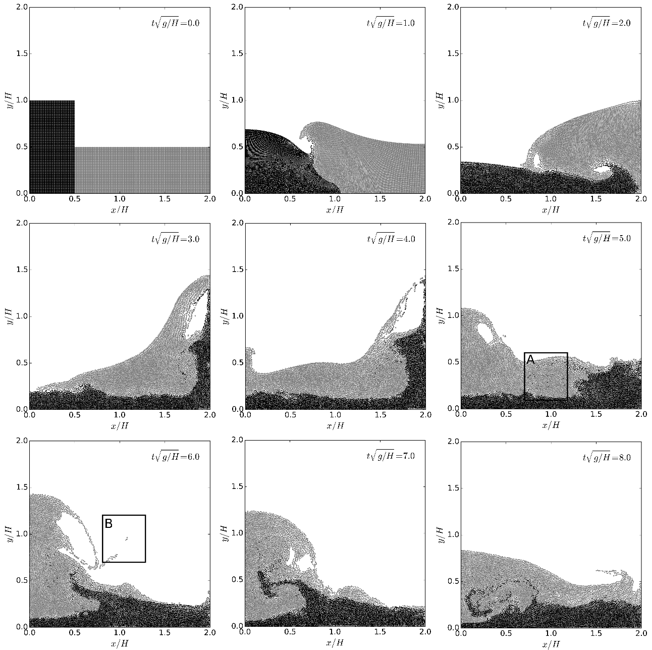
Figure 2: Evolution of the dam breaking test case $(Re=2000)$ calculated using the SPH approach ($h/H=1/32$, $h/\Delta r=2$); frames A and B (zoomed in Fig. 3) indicate regions where some single SPH particle droplets/solids appears and travel through the domain.

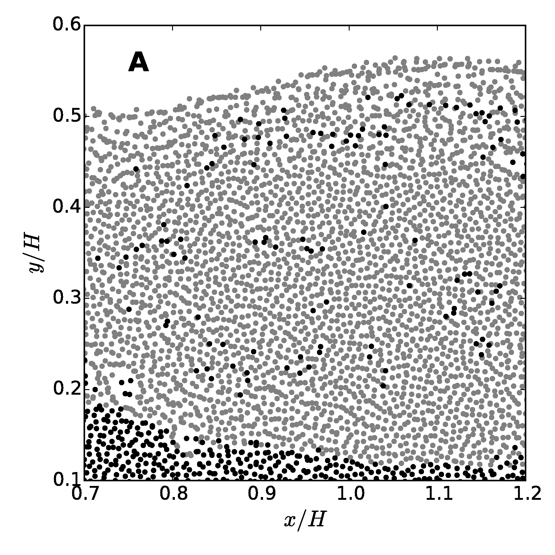
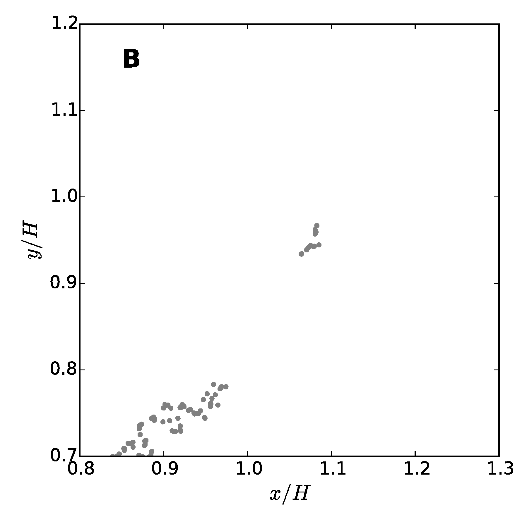
Figure 3: Zoom of the regions where single SPH particles droplets/solids appear and travel in the dam breaking test case simulation; frame A shows swarms of single particles of the denser phase within the lighter one; frame B presents the fragmentation of the free-surface.

From the physical point of view, in both: A and B cases, the single droplets could appear in the flow as an effect of the instabilities in the flow, e.g. Rayleigh-Taylor or Kelvin-Helmholtz in the case A, the Rayleigh-Plateau in the case B, and shear. However, in the case of the SPH modelling, the size of the single droplet is determined by the size of a single SPH particle. What is more, since the single SPH particle is represented by position (point), density and mass, the definition of the SPH particle size is not obvious. Although the mass of particle is usually fixed, the density can change which implies the change of the particle volume. Therefore, the physical interpretation of the process of appearance of single droplets is not evident. Probably, in most of the cases such a behaviour has to be interpreted as a numerical error related to the low-resolution, sub-kernel particle motion, or/and non-physical pressure pulsation in WCSPH or lack of volume conservation in ISPH. The problem is that the dense droplet swarms as presented in Fig. 3(A) or free-falling droplets, see Fig. 3(B), hitting (with high velocity) the free-surface can significantly modify the flow in the whole domain. Nevertheless, for further discussion, let us assume that the resolution is high enough to interpret appearance of the single particle droplet as a physically correct process. Is the motion of a single particle droplet physically correct? What is a diameter of such a droplet? What is an influence of the SPH numerical parameters such as $h$, $h/\Delta r$ or the shape of the kernel on the motion of the single particle?

4 Drag coefficient of single particle droplet/solid

In order to answer all raised questions about the motion of single droplet, we decided to perform a simple numerical experiment. We considered a cuboid of the edges’ sizes: $L_{x}=L$, $L_{y}=L$ and $L_{z}=2L$. The whole domain is filled with the fluid of density, $\varrho_{L}$. Since the hydrostatic pressure balances the effect of the gravitational acceleration, the system is at rest. At some point, we change the density of one particle (located centrally in the upper part of the domain) into the density of the solid/droplet particle, $\varrho_{S}$. Due to the gravity, the solid particle begins to fall. It accelerates to reach the terminal velocity $u_{T}$. The evolution of the described set-up is presented in Fig. 4.

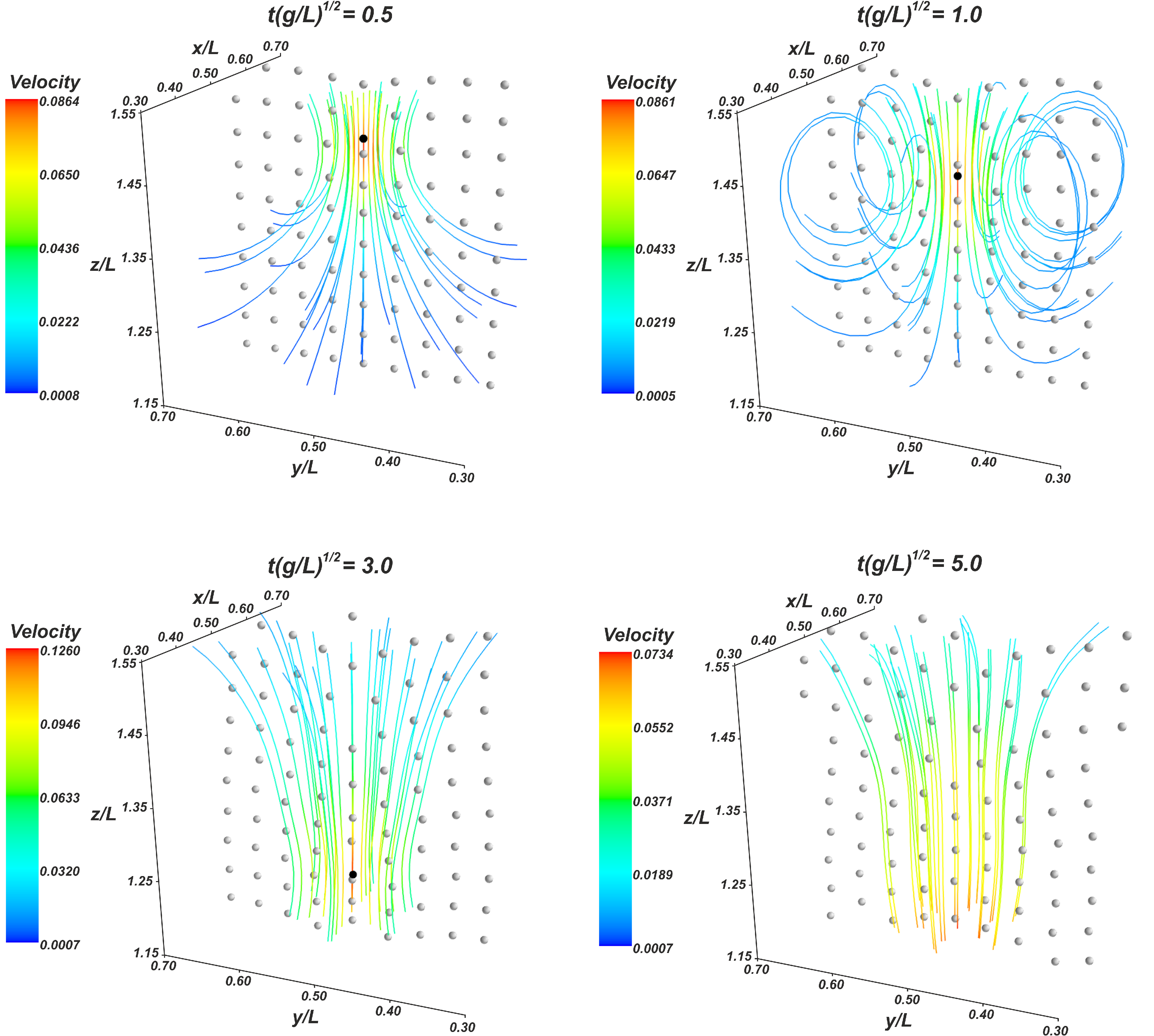
Figure 4: Results of the SPH modeling of single SPH particle solid (black one) falling down due to gravity; gray particles represent fluid; the streamlines are calculated using the Mayavi [25] plotting tool.

In reality, the solid object inserted into the liquid should move according to the relation

$$m\frac{d\mathbf{u}}{dt}=\mathbf{F}_{G}+\mathbf{F}_{B}+\mathbf{F}_{D},$$ (14)

where $\mathbf{F}_{G}=m\mathbf{g}$ is the gravitational force, $\mathbf{F}_{B}$ is the buoyancy force and $\mathbf{F}_{D}$ is the drag (lift forces are omitted). In general (from the Buckingham $\Pi$ theorem), the drag force can be expressed in the form

$$F_{D}=\frac{1}{2}\varrho_{L}\mathbf{u}^{2}AC_{D},$$ (15)

where $A$ is the cross sectional area of the body, while $C_{D}$ is the drag coefficient – a dimensionless number, which is dependent on the Reynolds number, see [22, 23] for details. Assuming that the considered body is sphere with the diameter $D$, the Reynolds number, defined as $Re=uD/\nu$, is low ($Re<1$ – Stokes flow). Hence, the drag coefficient takes a very elegant form [24]

$$C_{D}=\frac{24}{Re}.$$ (16)

For higher Reynolds numbers (including the turbulent flow), there are many different propositions of correlations between the drag coefficient and the Reynolds number, see [23] for review (for non-spherical particles see [26]). The most commonly used correlation which is reasonably for the Reynolds numbers up to $Re=800$ is the relationship proposed by Schiller and Naumann (1933) [27]

$$C_{D}=\frac{24}{Re}\left(1+0.15Re^{0.687}\right).$$ (17)

Assuming the Stokes regime of the flow, Eq. (16), the solution of Eq. (14) is

$$u(t)=\frac{D^{2}g}{18\mu}(\varrho_{S}-\varrho_{L})\left(1-e^{-\frac{18\mu}{D^{2}\varrho_{s}}t}\right),$$ (18)

which asymptotically approaches the terminal velocity

$$u_{T}=\frac{D^{2}g}{18\mu}(\varrho_{S}-\varrho_{L}).$$ (19)

The drag coefficient, for the terminal velocity, can be measured from the relationship

$$C_{D}=\frac{4}{3}\frac{gD}{u_{T}^{2}}\left(\frac{\varrho_{S}}{\varrho_{L}}-1\right).$$ (20)

It is important to note that Eqs. (18)-(20) explicitly depend on the diameter of the particle/droplet. This fact implies another question – what is the diameter of the SPH particle seen by the fluid. Taking into account the initial homogeneous distribution of particles, the intuitive diameter of particle is $D=\Delta r$. On the other hand, in the SPH modeling we have two characteristic sizes which determine the resolution: $\Delta r$ and $h$. The third option is the particle diameter $D_{\Omega}$ determined from the assumption of particle sphericity and a constant volume $\Omega=m/\varrho$

$$D_{\Omega}=\sqrt[3]{\frac{6}{\pi}\frac{m}{\varrho}}=\sqrt[3]{\frac{6}{\pi}}\Delta r.$$ (21)

Due to this ambiguity, we decided to consider all three possibilities.

In order to check whether the SPH method can give proper predictions of velocities when single particle/droplets are considered, we decided to perform a set of simulations for different density ratios, $\varrho_{S}/\varrho_{L}$ and two different resolutions: $h/L=1/16$ and $h/L=1/32$. In all simulations we decided to use the Wendland kernel and $h/\Delta r=1.5625$. The dimensionless velocities calculated with the SPH method compared with the analytical predictions, Eq. (18), are presented in Fig. 5.

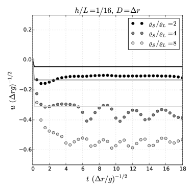
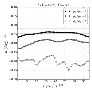
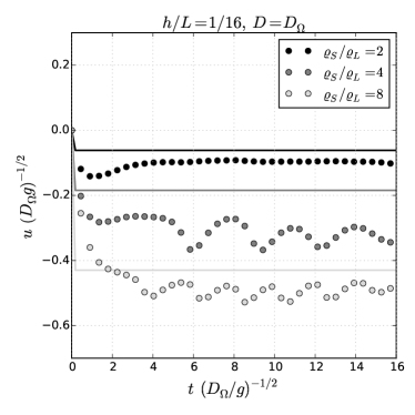
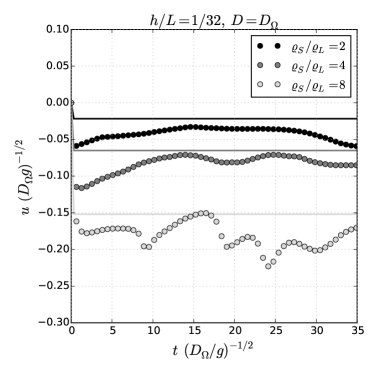
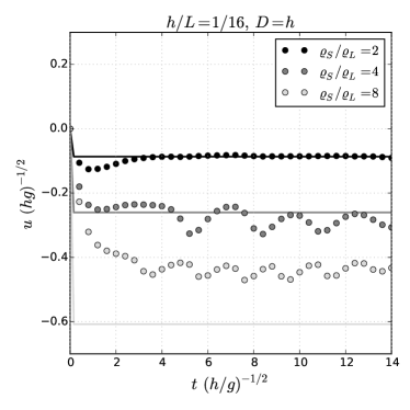
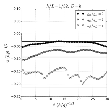
Figure 5: Vertical velocity of solid particle falling down within fluid; the results obtained using the SPH approach (dots), and compared with the analytical predictions (solid lines), for different values of $h/L$ and different assumptions about the SPH particle diameter $D$.

The obtained results show very high oscillations related to the interactions with the internal structure of the liquid, consisting of finite number of the SPH particles. However, the most interesting is a much better agreement with the reference solution if we assume that $D=h$. For $D=D_{\Omega}$ the results are slightly less accurate, while for $D=\Delta r$ we obtained the worst agreement with Eq. (18).

In the next step, we decided to calculate the drag coefficient $C_{D}$ for different density ratios which corresponds to different Reynolds numbers $Re$, and then compare it with the analytical Stokes (1851), Eq. (16), and experimental Schiller and Naumann (1933), Eq. (17) correlations. The results obtained for two different resolutions: $h/L=1/16$ and $1/32$, and three different assumptions about the diameter of particle: $D=\Delta r$, $D_{\Omega}$ and $h$, are presented in Fig. 6.

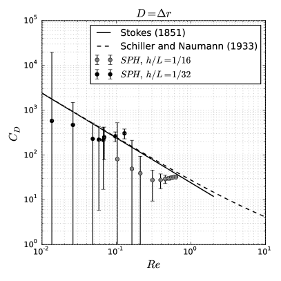
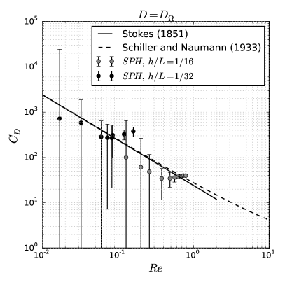
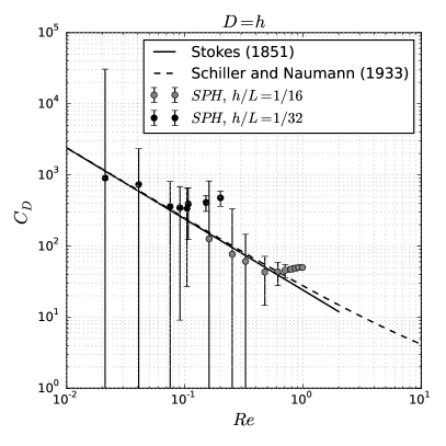
Figure 6: Drag coefficient $C_{D}$ of falling particle as function of the Reynolds number $Re$ calculated using the SPH approach (dots); the SPH results are compared with the analytical (solid line) and experimental predictions (dashed line) for different assumptions about the particle diameter $D$.

The first conclusion from these results is the underestimation of the drag coefficient in the case of $D=\Delta r$. The second conclusion is a very high standard deviation of the calculated drag coefficients for relatively slow particles, which is the result of the oscillations presented in Fig. 5. The third outcome is a high mismatch between the SPH calculations and the reference correlations for relatively fast particles (these with small errorbars).

Therefore, taking into account the above-mentioned conclusions, the question about the physical correctness of the single particle droplets/solids should be answered: this motion is highly affected by SPH nodes (particles) and therefore non-physical. However, on the other hand, trying to be more open-minded, since the results obtained for relatively low velocities (these with large errorbars in Fig. 6) are with (high) margin of error in agreement with the reference data, we could potentially model large swarms of solid particles (e.g. sediments) interpreting the obtained results statistically.

However, very intriguing is the question about the diameter of the particle. The obtained results show much better agreement with the reference data for $D=h$ and $D=D_{\Omega}$, than $D=\Delta r$. Since the smoothing length can be chosen independently from the particle mass and density (for given $h$ mass is determined by the parameter $h/\Delta r$), a good agreement for $D=h$ is very surprising. In order to check whether this fact is just a coincidence, we decided to investigate the influence of the $h/\Delta r$ parameter on the resulting drag coefficient. The simulations were performed for three different values of $h/L=1/16$, $1/32$ and $1/64$, four different values of $h/\Delta r=1.5625$, $1.75$, $1.9375$, $2.125$ and constant $\varrho_{S}/\varrho_{L}=6$.

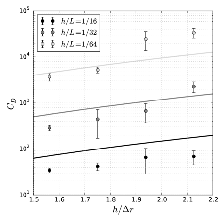
Figure 7: Influence of $h/\Delta r$ parameter on the value of drag coefficient; comparison of results from simulations (dots) with the analytical predictions (lines), see Eq. (22).

The obtained results are presented in Fig. 7. The solid lines denote the expected, analytical (Stokes regime) dependency between the drag coefficient, $C_{D}$, and the parameter $h/\Delta r$

$$C_{D}=\frac{72\mu^{2}\pi}{g(\varrho_{S}-\varrho_{L})\varrho_{L}h^{3}}\left(\frac{h}{\Delta r}\right)^{3}.$$ (22)

Since both the SPH calculations and the analytical curve, Eq. (22), shows a similar upward trend with an increase in $h/\Delta r$, this indicates that the SPH particle diameter seen by fluid can not be $h$ – in fact, it is $D_{\Omega}$.

5 Conclusions

Our simple numerical experiment yields important information on how single SPH particles should be viewed. The obtained results clearly indicate that movement of single SPH particles can not be considered as physically correct. Simulations of solid particles falling down in liquid showed that its behavior is highly affected by interactions with particles representing fluid. This issue is reflected in oscillations of velocity. Comparison of values of drag coefficient with the analytical and the experimental predictions also does not speak in favour of such a modeling using the SPH framework. While numerical results for relatively slow particles are within margin of error, agreement decreases significantly for faster ones. This leads towards conclusion, that in SPH simulations of multiphase flows, movement of single SPH particle solids/droplets should be regarded as numerical error, not psychical phenomenon. Furthermore ambiguities concerning size of single SPH particle has been cleared out. Among three candidates for diameter seen by fluid, i.e. $h$, $\Delta r$ and $D_{\Omega}$, the last one obtained from assumption of sphericity and constant volume $\Omega=m/\varrho$, was proved to be the best estimation.

References

- [1] Monaghan JJ. Smoothed Particle Hydrodynamics. Annual Review of Astronomy and Astrophysics 1992; 30 : 543-574.
- [2] Monaghan JJ. Smoothed Particle Hydrodynamics and its diverse applications. Annual Review of Fluid Mechanics 2012; 44 : 323-346.
- [3] Violeau D. Fluid Mechanics and the SPH Method: Theory and Applications. Oxford University Press, 2012.
- [4] Colagrossi A, Landrini M. Numerical simulation of interfacial flows by smoothed particle hydrodynamics. Journal of Computational Physics 2003; 191 : 227-264.
- [5] Grenier N, Antuono M, Colagrossi A., Le Touzé D, Allesandrini B. An Hamiltonian interface SPH formulation for multi-fluid and free-surface flows. Journal of Computational Physics 2009; 228 : 8380-8393.
- [6] Szewc K, Pozorski J, Minier JP. Spurious interface fragmentation in multiphase Smoothed Particle Hydrodynamics. International Journal for Numerical Methods in Engineering 2015; accepted.
- [7] Szewc K, Pozorski J, Minier JP. Simulations of single bubbles rising through viscous liquids using Smoothed Particle Hydrodynamics. International Journal of Multiphase Flow 2013; 50 : 98-105.
- [8] Wieth L, Christian L, Kurz W, Braun S, Koch R, Bauer HJ. Numerical modeling of an aero-engine bearing chamber using the meshless smoothed particle hydrodynamics method. Proceedings of ASME Turbo Expo 2015: Turbine Technical Conference and Exposition; GT2015-42316.
- [9] Wieth L, Braun S, Koch R, Bauer HJ, Kelemen K, Schuchmann HP. Smoothed Particle Hydrodynamics (SPH) simulation of a high-pressure homogenizer. Proceedins of the 9th SPHERIC International Workshop 2015, Paris.
- [10] SPHERIC - SPH European Research Interest Community. https://wiki.manchester.ac.uk/spheric/.
- [11] Wendland H. Piecewise polynomial, positive definite and compactly supported radial functions of minimal degree. Advances in Computational Mathematics 1995; 4 : 389-396.
- [12] Szewc K, Pozorski J, Minier JP. Analysis of the incompressibility constraint in the SPH method. International Journal for Numerical Methods in Engineering 2012; 92 343-369.
- [13] Koshizuka S, Nobe A, Oka Y. Numerical analysis of breaking waves using the moving particle semi-implicit method. International Journal for Numerical Methods in Fluids 1998; 26 : 751-769.
- [14] Szewc K, Tanière A, Pozorski J, Minier JP. A study on application of smoothed particle hydrodynamics to multi-phase flows. International Journal of Nonlinear Sciences and Numerical Simulations 2012; 13 : 383-395.
- [15] Hu XY, Adams NA. A multi-phase SPH method for macroscopic and mesoscopic flows. Journal of Computational Physics 2006; 213 : 844-861.
- [16] Monaghan JJ. Smoothed particle hydrodynamics. Reports on Progress in Physics 2005; 68 : 1703-1759.
- [17] Cummins S, Rudman M. An SPH projection method. Journal of Computational Physics 1999; 152 : 584-607.
- [18] Hu XY, Adams NA. An incompressible multi-phase sph method. Journal of Computational Physics 2007; 227 : 264-278.
- [19] Shao S, Lo EYM. Incompressible SPH method for simulating Newtonian and non-Newtonian flows with a free surface. Advances in Water Resources 2003; 26 : 787-800.
- [20] Xu R, Stansby P, Laurence D. Accuracy and stability in incompressible sph based on the projection method and a new approach. Journal of Computational Physics 2009; 228 : 6703-6725.
- [21] Rafiee A, Cummins S, Rudman M, Thiagarajan K. Comparative study on the accuracy and stability of SPH schemes in simulating energetic free-surface flows. European Journal of Mechanics - B/Fluids 2012; 36 : 1-16.
- [22] Batchelor GK. An Introduction to Fluid Dynamics. Cambridge University Press, 2000.
- [23] Crowe CT, Schwarzkopf JD, Sommerfeld M, Tsuji Y. Multiphase Flows with Droplets and Particles. CRC Press, Taylor & Francis Group, 2012.
- [24] Stokes GG. On the effect of the internal friction of fluids on the motion of pendulums. Transactions of the Cambridge Philosophical Society 1851; 9 : 8-106.
- [25] Ramachandran P, Varoquaux G. Mayavi: 3D visualization of scientific data. IEEE Computing in Science & Engineering 2011; 13 : 40-51.
- [26] Ouchene R, Khalij M, Tanière A, Arcen B. Drag, lift and torque coefficients for ellipsoidal particles: From low to moderate particle Reynolds numbers. Computers & Fluids 2015; article in press.
- [27] Schiller I, Naumann A. Fundamental calculations in gravitational processing. Vereines Deutscher Ingenieure 1933; 77 : 318-20.