Constraining Neutrino mass using the large scale HI distribution in the Post-reionization epoch
Abstract
The neutral intergalactic medium in the post reionization epoch allows us to study cosmological structure formation through the observation of the redshifted 21 cm signal and the Lyman-alpha forest. We investigate the possibility of measuring the total neutrino mass through the suppression of power in the matter power spectrum. We investigate the possibility of measuring the neutrino mass through its imprint on the cross-correlation power spectrum of the 21-cm signal and the Lyman-alpha forest. We consider a radio-interferometric measurement of the 21 cm signal with a SKA1-mid like radio telescope and a BOSS like Lyman-alpha forest survey. A Fisher matrix analysis shows that at the fiducial redshift , a 10,000 hrs 21-cm observation distributed equally over 25 radio pointings and a Lyman-alpha forest survey with 30 quasars lines of sights in , allows us to measure at a level. A total of 25,000 hrs radio-interferometric observation distributed equally over 25 radio pointings and a Lyman-alpha survey with will allow to be measured at a level. This corresponds to an idealized measurement of at the precision of and at level.
keywords:
cosmology: theory – large-scale structure of Universe - cosmology: diffuse radiation – cosmology: neutrino mass1 Introduction
It has been established from neutrino oscillation experiments that neutrinos have mass. There are profound implications of these particles being massive and cosmological observations are expected to put strong constrains on neutrino physics. Several cosmological probes are used in this regard (Lesgourgues et al., 2013). We believe that at least two of the three species of neutrinos are non-relativistic today. Neutrinos are in expected to be in thermal equilibrium with CMBR in the early Universe and their number is fixed. Accordingly their fractional contribution to the present day matter budget is given by where =eV (Lesgourgues & Pastor, 2012, 2014) with denoting the mass of each neutrino species. When the temperature of the universe is very high they can be treated as a part of radiation and after the CMB temperature drops below their masses, they can contribute to the matter density of the Universe. The free streaming behaviour of neutrinos causes them to wipe out fluctuations on scales smaller than the horizon scale when the neutrinos became non-relativistic (Hu & Eisenstein, 1998; Eisenstein & Hu, 1999; Lesgourgues et al., 2013). The free-streaming comoving vector is given by where denotes the free-streaming speed. When neutrinos are relativistic, this coincides with the horizon scale, and when neutrinos become non-relativistic at (Agarwal & Feldman, 2011) it becomes
For modes neutrinos behave like usual dark matter and there is no suppression of power. Modes with have neutrino perturbations wiped out and consequently CDM power spectrum is also suppressed. Cosmological measurement of neutrino mass (Croft et al., 1999a; Hannestad, 2003; Pritchard & Pierpaoli, 2008; Gratton et al., 2008; Vallinotto et al., 2009; Palanque-Delabrouille et al., 2015; Di Valentino et al., 2015; Giusarma et al., 2014; Allison et al., 2015; Chen et al., 2016) depends directly on the level of precision at which this suppression of power in the matter power spectrum can be detected. Whereas CMBR gives stringent constraints on neutrino mass (Lesgourgues et al., 2006; Oyama et al., 2013; Pan & Knox, 2015; Planck Collaboration et al., 2014, 2015) it is necessary to obtain measurements from the low redshift Universe. Matter power spectrum for is highly non-linear and neutrino mass measurements have degeneracies with competition from dark energy (Hannestad, 2005).
Mapping the neutral hydrogen distribution (HI) in the post-reionization epoch using the observation of the redshifted 21 cm signal towards measurement of the matter power spectrum has been studied as a means to measure neutrino mass (McQuinn et al., 2006a; Pritchard & Pierpaoli, 2008; Oyama et al., 2013; Shimabukuro et al., 2014; Liu et al., 2016; Oyama et al., 2016). At redshifts , HI responsible for the 21 cm signal lies predominantly in the Damped Lyman Alpha (DLA) clouds (Wolfe et al., 2005) and the diffuse collective 21 cm emission from these clouds form a background in radio observations. The redshifted 21-cm diffuse emission from the post-reionization epoch is well modelled using a constant neutral fraction (Storrie-Lombardi et al., 1996; P’eroux et al., 2003), and a bias function (Bagla et al., 2010; Guha Sarkar et al., 2012). The diffuse neutral gas distribution in the same redshift range can also be probed using the distinct absorption features of the Lyman-alpha forest (Rauch, 1998). Large astrophysical foregrounds (Di Matteo et al., 2002; Santos et al., 2005; Gleser et al., 2008; Liu et al., 2009; Ghosh et al., 2011; Alonso et al., 2015) come in the way of detecting the 21 cm signal. The cross correlation of the 21 cm signal with other cosmological probes like the Lyman-alpha forest and Lyman-Break galaxies, has been proposed as a viable way (Guha Sarkar et al., 2011; Guha Sarkar & Datta, 2015; Villaescusa-Navarro et al., 2015a) to mitigate the effect of foregrounds. The flux through the Lyman-alpha forest and the redshifted 21 cm signal can both be modeled as biased tracers of the underlying dark matter distribution and are expected to be correlated (McDonald, 2003; Bagla et al., 2010; Guha Sarkar et al., 2012; Villaescusa-Navarro et al., 2014). The cross-correlation signal is a direct probe of the matter power spectrum over a large redshift range in the post reionization epoch.
In this paper we investigate the constraints on total neutrino mass using the cross correlation of the Lyman-alpha forest and the 21-cm signal from the post reionization epoch. The suppression of power on scales allows us to constrain the neutrino mass. In this paper we constrain the parameters and using the cross-correlation signal. These are the only two free parameters in our analysis. The values of are fixed to their fiducial values as obtained from (Planck Collaboration et al. (2015)Table 4: TT + lowP) for this analysis. varies but is not treated as a free independent parameter. We consider a future radio interferometric observation of the 21 cm using a telescope like SKA1-mid 111https://www.skatelescope.org/ and a BOSS 222https://www.sdss3.org/surveys/boss.php like Lyman-alpha forest survey for obtaining predictions for bounds on the parameters.
2 Cross correlation signal and estimation of Neutrino mass
The cross-correlation of the redshifted 21-cm signal and the transmitted flux through the Lyman-alpha forest has been proposed and studied as a cosmological probe of structure formation and background evolution in the post-reionization epoch (Guha Sarkar & Datta, 2015). The two signals of interest owe their origins to neutral hydrogen (HI) in distinct astrophysical systems at redshifts but are expected to be correlated on large scales.
Bulk of the HI in the post-reionization epoch is believed to be housed in the dense self-shielded DLA systems. These clumps are the dominant source of the 21-cm emission in this epoch. The signal from individual DLA sources is rather weak and resolving individual sources is also rather unfeasible. The collective emission from the clouds, however form a diffuse background in all radio observations at observing frequencies less than MHz. Tomographic imaging using the low resolution intensity mapping of this diffuse background radiation is a potentially rich probe of cosmology (Bharadwaj & Sethi, 2001; Loeb & Wyithe, 2008; Chang et al., 2008; Wyithe, 2008; Bharadwaj et al., 2009; Wyithe & Loeb, 2009; Camera et al., 2013; Bull et al., 2015).
Along a line of sight traversing a HI cloud at redshift the CMBR brightness temperature changes from to owing to the emission/absorption corresponding to the spin flip Hyperfine transition at MHz in the rest frame of the gas.
| (1) |
where is the 21-cm optical depth and is the spin temperature (Furlanetto et al., 2006). The quantity of interest in radio observations at a frequency is the excess brightness temperature redshifted to the observer at present. This is given by
| (2) |
Writing , where is the comoving distance corresponding to , we have the fluctuations in given by (Bharadwaj & Ali, 2004) , where
| (3) |
and
| (4) |
Here denote the mean neutral fraction, denotes the HI density fluctuations and is a function that takes into account the fluctuations of the spin temperature assuming it to be related to the HI fluctuations. The peculiar velocity of the gas, introduces the anisotropic term .
In the post reionization epoch one has whereby the 21 cm signal is seen in emission and we have
| (5) |
In Fourier space the fluctuation in 21-cm excess brightness temperature is denoted by and is given by
| (6) |
where is the Fourier transform of the dark matter over density and we have assumed that the peculiar velocity is sourced by dark matter over density. The quantity is similar to the redshift space distortion (Hamilton, 1998) parameter and . The redshift dependent quantity is given by where denotes a bias that relates the HI fluctuations in Fourier space to the underlying dark matter fluctuations as . The 21 cm bias has been studied in several independent studies (Khandai et al., 2009; Marín et al., 2010; Guha Sarkar et al., 2012). The small scale fluctuations clearly have a scale dependent bias which grows monotonically with . There is also some additional scale dependence owing to fluctuations in the ionizing background (Wyithe & Loeb, 2009). Numerical simulations show that on large scales the bias is however found to be a constant increasing only with redshift (Khandai et al., 2009; Marín et al., 2010; Guha Sarkar et al., 2012). We adopt a linear bias model (Guha Sarkar et al., 2012) in this work. It is important to note that in cosmologies with massive neutrinos HI is more clustered. This is an additional effect which occurs because we fundamentally believe that the gas is contained in halos and halos are rarer in models with neutrino mass and are thereby more biased (Massara et al., 2015). This enhances the 21-cm power spectrum by a roughly scale independent factor of at (Villaescusa-Navarro et al., 2015b).
Whereas the dense clumpy HI sources the 21 cm emission, the diffuse intergalactic HI in the post reionization epoch also produces distinct absorption lines in the spectra of background quasars namely the Lyman-alpha forest (Hui & Gnedin, 1997; Kim et al., 2007). The 21 cm signal and the Lyman-alpha forest arises from two distinct astrophysical systems. Bulk of the 21 cm emission comes from the dense HI clouds which are self shielded from the ionizing photons. The Lyman-alpha forest, on the other hand consists of absorption lines in the Quasar spectra which originates from tiny fluctuations in the low density diffuse HI along the line of sight. The Flux through the Lyman-alpha forest is modeled using the fluctuating Gunn-Peterson approximation (Gunn & Peterson, 1965; Bi & Davidsen, 1997)
| (7) |
where is related to the slope of the temperature density relationship as , and (Kim et al., 2007) is a redshift dependent parameter depending on several astrophysical and cosmological parameters like the photo-ionization rate, IGM temperature and the evolution history (Croft et al., 1998, 1999b). The relationship between the observed flux through the Lyman-alpha forest and the underlying dark matter distribution is non-linear(Slosar et al., 2011). However, on large scales the smoothed Lyman-alpha forest flux traces the dark matter fluctuations (Viel et al., 2002; Saitta et al., 2008; Slosar et al., 2009) via a bias. The precise analytic understanding about the bias is not very robust and has been studied under certain approximations. However, a linear bias model is largely supported by numerical simulations of the Lyman-alpha forest (McDonald, 2003).
The fluctuations of the flux through the Lyman-alpha forest can hence be related to the dark matter fluctuations in Fourier space as
| (8) |
The parameters are independent of one another and depend on , and the flux probability distribution function. The predictions for from particle-mesh simulations indicate that increasing the smoothing length has the effect of lowering the value of which is ideally set by choosing the smoothing scale at the Jean’s length which is in turn sensitive to the IGM temperature. We adopt the values from simulations of Lyman-alpha forest (McDonald, 2003).
Being tracers of the underlying dark matter distribution the Lyman-alpha forest and 21 cm signal are expected to be correlated. The cross correlation of the Lyman-alpha forest and the 21cm signal has been proposed as a cosmological probe (Guha Sarkar et al., 2011; Guha Sarkar & Datta, 2015). Apart from mitigating the serious issue of 21 cm foregrounds, the cross correlation if detected, ascertains the cosmological origin of the signal as opposed to the auto correlation 21 cm signal. Several advantages of the cross-correlation have been studied in earlier works (Guha Sarkar & Datta, 2015). The 3D cross correlation power spectrum is defined through
| (9) |
with
| (10) |
where is the dark matter power spectrum.
Observationally the Lyman-alpha forest survey as well as radio observations of the 21 cm signal will probe certain volumes of the Universe. The cross-correlation can however be computed only in the overlapping region denoted by . The Lyman-alpha surveys typically shall cover a larger volume and thus is set by the 21-cm observations. If be the observational bandwidth of the 21 cm observation and if is the angular patch that the radio telescope probes, then .
The observed 21 cm signal denoted by shall include a noise term and may be written as
| (11) |
Similarly the observed Lyman-alpha forest transmitted flux fluctuation in Fourier space may be written as
| (12) |
which involves a convolution of the three dimensional field with a normalized sampling function in Fourier space , and denotes a pixel noise contribution. The sampling function relates the one dimensional Lyman-alpha forest skewers to the 3D field and is given by
| (13) |
with a set of weight functions that are used to maximize the SNR and is used to normalize . The sum extends over all the QSO locations in the field. The error in measurement of the cross power spectrum is hence given by , where
| (14) |
where denotes the one dimensional power spectrum of Lyman-alpha forest flux fluctuations
| (15) |
Here and denotes the noise power spectrum for 21 cm observation and the Lyman-alpha forest respectively and denotes the power spectrum of the weight functions. The quantity is the number of available Fourier modes and is given by
| (16) |
The noise power spectrum for the 21 cm observations and the Lyman-alpha forest depend on the specific observational parameters. For radio-interferometric observation of the 21 cm signal the noise power spectrum is a function of the mode being probed and the observation frequency and is given by (McQuinn et al., 2006b; Wyithe et al., 2008)
| (17) |
where, denotes the effective collecting area of a single antenna, and is the total observation time for a single pointing. The system temperature is denoted by . If denotes the total number of antennae and (Datta et al., 2007; Geil et al., 2011; Villaescusa-Navarro et al., 2015a) is the normalized baseline distribution function.
For the Lyman-alpha forest observations, the noise power spectrum is given by (McQuinn & White, 2011)
| (18) |
where is the average quasar number density in the field given by for a total of QSO spectra in the field of view and is the variance of the pixel noise with
| (19) |
The signal to ratio in a pixel of size , with matched to the frequency smoothing scale of the 21 cm observation is considered to be held at a constant average value of . To make error estimates for the two parameters and we use the Fisher matrix with elements
| (20) |
where and can take values and . The Cramer-Rao bound gives a limit on the the theoretical errors on the parameter as which we use in this paper.
3 Results and Discussion
We have assumed a fiducial cosmological model with = (Planck Collaboration et al., 2015) for this analysis. The fiducial redshift is chosen since the quasar distribution peaks in the redshift range . At this fiducial redshift the Lyman-alpha forest spectrum can be measured in an approximate range . This is owing to the fact that part of the quasar spectrum blue-ward of the Lyman-alpha emission and red-ward of the Ly- line has to eliminated to avoid the quasar proximity effect and contamination from Ly- and other metal lines respectively. A high quasar density is required for the cross-correlation to be measured at high level of sensitivity. We consider a BOSS like Lyman-alpha forest survey with a quasar density of with an average sensitivity for the measured spectra. The BOSS survey covers a large part of the sky with a transverse coverage of . The volume probed by the Lyman-alpha forest is hence given by with and . We note, however that the cross-correlation can only be computed only in the overlapping volume between the Lyman-alpha forest survey and 21cm survey volume which is expected to be much smaller.
We consider an 21cm intensity mapping experiment using a radio interferometer with specifications roughly following that of SKA1-mid 333http://www.skatelescope.org/wp-content/uploads/2012/07/SKA-TEL-SKO-DD-001-1_BaselineDesign1.pdf. The radio interferometer shall operate in frequency range from MHz to GHz. The fiducial redshift of corresponds to a frequency of falls in this frequency range. We assume the array to be composed of a total of dish like antennae. Each individual antenna is of diameter m with an antenna efficiency of . We assume that the distribution of the antennae is mostly condensed to a central core with , , , and of the total antennae are within km, km, km, and km radius respectively with density of antennae falling off radially as an inverse square power law (Villaescusa-Navarro et al., 2014). This allows us to compute the normalized baseline distribution function. It is evident that there can not be any baselines below . Typical intensity mapping experiments aim towards higher power spectrum sensitivity at large scales. The telescope design supports this, since the telescopes are mostly distributed in a central region. The baseline coverage at very small non-linear scales is poor. We assume the system temperature to be K at observational frequency of MHz. Further, the telescope is assumed to have a band width.
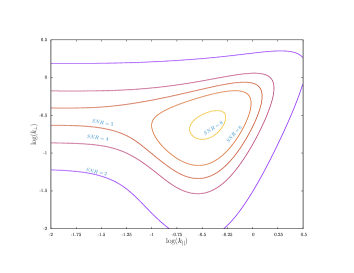
Figure (1) shows the signal to noise ratio for the cross-correlation signal in the plane. We have considered a observation of the 21-cm signal in a single pointing of the telescope. We find that a statistically significant detection of the cross-correlation signal at a SNR is possible in the range and . The anisotropy in the space owes its origin to the redshift space distortion effects and the preferential sensitivity of the noise in the space. We have assumed here that a perfect foreground subtraction has been achieved. Foreground residuals are expected to degrade the SNR. The issue of foreground removal has been discussed later. The low sensitivity at small baselines owes it origin to cosmic variance whereas the sensitivity at large scales is dictated by instrument noise.
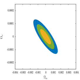
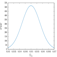
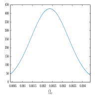
We next, look at the results of the Fisher matrix analysis towards constraining the parameters . Figure (2) shows the confidence ellipses at , and levels. We have considered a total 21 cm observation for 25 pointings of radio telescope each corresponding to a observation. The Lyman-alpha forest survey is assumed to have QSO number density of where each spectrum is measured at an average pixel noise level. We find that for these observational parameters, and can be measured at and respectively. Figure (2) also shows the marginalized probability distribution for the parameters and .
The SKA1-mid kind of radio interferometer considered here has a angular coverage of at redshift of . This is much smaller than volume covered by the Lyman-alpha survey. The BOSS Lyman-alpha survey covers a much larger volume than a typical 21 cm observation. A significant part of the Lyman-alpha survey volume can be used in the cross-correlation by considering multiple pointings of the radio interferometer. We keep the total observation time fixed at but now consider radio pointings each of duration. Further we consider the possibility of dividing the total observing time into 100 pointings.The results show a clear improvement in the constraints. We tabulate all the results in tables (1) and ( 2). This implies that for a QSO survey with a number density and with SKA like instrument, it is more advantageous to distribute the total observation time over as many fields of views as possible instead of deep imaging of a single radio field.
| Parameter | Fiducial | Error | Error | Error |
|---|---|---|---|---|
| value | 25 pointings | 50 pointings | 100 pointings | |
| 0.315 | .361 | 0.280 | 0.222 | |
| 0.315 | 0.310 | 0.237 | 0.184 | |
| 0.315 | 0.298 | 0.227 | 0.176 | |
| 0.315 | 0.296 | 0.227 | 0.174 | |
| 0.315 | 0.292 | 0.222 | 0.171 |
| Parameter | Fiducial | Error | Error | Error |
|---|---|---|---|---|
| value | 25 pointings | 50 pointings | 100 pointings | |
| 7.10 | 20.70 | 16.53 | 13.81 | |
| 1.42 | 6.47 | 5.21 | 4.25 | |
| 2.13 | 3.73 | 3.00 | 2.45 | |
| 2.37 | 3.25 | 2.61 | 2.13 | |
| 2.84 | 2.57 | 2.07 | 1.68 |
Up-to this point our analysis is focused on the estimates of the parameters HI 21 cm intensity mapping using (with SKA1-mid) and Lyman-alpha (BOSS) surveys, with some specific observational parameters (i.e, QSO density, number of antennae,and time of observations). In the next analysis our interest is focused on the variation of the error estimates if the above mentioned observational parameters are changed within the known possible range.
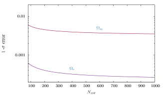
We first consider the effect of the variation of number of antennae from 100 to 1000 keeping the time of observation and QSO density ( ) unchanged. The total 10000 hrs time is hence divided over 25 radio pointings. The collecting area and resolution of the radio telescopes will increase with the number of antennae (keeping the dishes identical) . Figure (3) shows the error bound on varying with the number of antennas in the radio array. We find that there is no significant improvement in the constraints when number of antennas are increased beyond 350 and, the error bound saturates to a limit set by cosmic variance and the parameters of the Lyman-alpha survey.
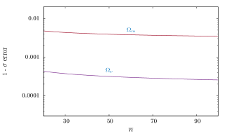
The noise contribution from the Lyman-alpha forest power spectrum measurement depends on the number density of Quasars in the survey. Figure (4) represents the improvement of 1 error in the estimation of parameters due to the of variation QSO density (). In this case we find that beyond the decline of the error is very slow and the cosmic variance limit is asymptotically reached.
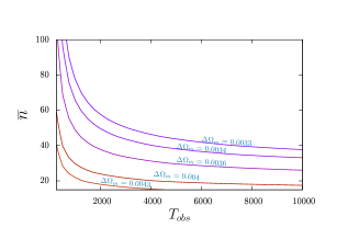
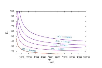
For a more practical scenario it is useful to investigate the optimal observational strategy. We characterize the radio observation with the time of observation and Lyman-alpha forest survey with the quasar number density in the survey with high SNR spectra. Figure (5) shows the contours of constant 1 errors of for a single pointing radio observation. The bottom left corresponds to large observational noise owing to small quasar number density and small time of observation. The top right corner corresponds to large quasar density and long duration radio observation. The error in the parameters show a decrease as one moves from the bottom left to the top right corner through the contours. However, beyond a point there is no further improvement and this corresponds to the cosmic variance limit. In this limit the parameter can be measured at a level and can be measured at . Further improvement is only possible through increase of the number of pointings which increases the survey volume and the errors scale as . A total of 25,000 hrs radio observation distributed equally over 25 pointings and a Lyman-alpha survey with will allow to be measured at a level. This corresponds to a measurement of at the precision of and at . Our general observation is that there should be greater emphasis of increasing survey volumes through bigger bandwidths or using smaller dishes and considering multiple fields of views against extremely deep surveys in small fields. This shall make the constraints parameters stronger. we however note that 25,000 hrs observation in 25 pointings is a rather unfeasible observational strategy. In this idealized survey it is possible to even look into the mass hierarchy for neutrinos. However, Several observational issues poses severe problems towards detection of the signal. The crucial issue as regarding the 21 cm signal, is the issue of foregrounds. Foregrounds like the galactic synchrotron radiation and extra galactic point sources are several orders of magnitude larger than the cosmological 21 cm signal. Further, man made RFIs (Ellingson, 2005) also contaminate the signal severely. Several foreground subtraction methods have been proposed. We note that though foreground subtraction is crucial towards measuring the 21 cm signal, these contaminants appear as noise in the cross-correlation and foreground residuals even of the same order of magnitude as the signal shall not entirely inhibit the detection of the cross-correlation signal unlike the unlike the auto correlation. Assuming a fiducial model with we find that if we have a foreground residual of the 21-cm signal at 200% of the signal itself then the constraint on degrades from to . Further, if the Lyman- forest pixel noise is at , the constaint on neutrino mass degrades to .
The Lyman-alpha forest surveys require very high SNR measurement of a large number of spectra for high precision detection of the cross-correlation signal which is necessary for obtaining stringent bounds on the neutrino mass. Further, one has to worry about several other observational issues like the effect of Galactic super wind. contamination from other metal lines etc. We conclude by noting that with future radio-observations of the cosmological redshifted 21-cm signal and Lyman-alpha forest surveys, it is possible to measure neutrino mass at a high level of precision using the cross-correlation power spectrum. We predict that the bounds obtained from such a measurement shall be competitive with other probes.
4 Acknowledgements
TGS would like to acknowledge the Department of Science and Technology (DST), Government of India for providing financial support through the project SR/FTP/PS-172/2012.
References
- Agarwal & Feldman (2011) Agarwal S., Feldman H. A., 2011, MNRAS, 410, 1647
- Allison et al. (2015) Allison R., Caucal P., Calabrese E., Dunkley J., Louis T., 2015, PRD, 92, 123535
- Alonso et al. (2015) Alonso D., Bull P., Ferreira P. G., Santos M. G., 2015, MNRAS, 447, 400
- Bagla et al. (2010) Bagla J. S., Khandai N., Datta K. K., 2010, MNRAS, 407, 567
- Bharadwaj & Ali (2004) Bharadwaj S., Ali S. S., 2004, MNRAS, 352, 142
- Bharadwaj & Sethi (2001) Bharadwaj S., Sethi S. K., 2001, Journal of Astrophysics and Astronomy, 22, 293
- Bharadwaj et al. (2009) Bharadwaj S., Sethi S. K., Saini T. D., 2009, PRD, 79, 083538
- Bi & Davidsen (1997) Bi H., Davidsen A. F., 1997, ApJ, 479, 523
- Bull et al. (2015) Bull P., Ferreira P. G., Patel P., Santos M. G., 2015, ApJ, 803, 21
- Camera et al. (2013) Camera S., Santos M. G., Ferreira P. G., Ferramacho L., 2013, Physical Review Letters, 111, 171302
- Chang et al. (2008) Chang T., Pen U., Peterson J. B., McDonald P., 2008, Physical Review Letters, 100, 091303
- Chen et al. (2016) Chen Y., Ratra B., Biesiada M., Li S., Zhu Z.-H., 2016, preprint, (arXiv:1603.07115)
- Croft et al. (1998) Croft R. A. C., Weinberg D. H., Katz N., Hernquist L., 1998, ApJ, 495, 44
- Croft et al. (1999a) Croft R. A. C., Hu W., Davé R., 1999a, Physical Review Letters, 83, 1092
- Croft et al. (1999b) Croft R. A. C., Weinberg D. H., Pettini M., Hernquist L., Katz N., 1999b, ApJ, 520, 1
- Datta et al. (2007) Datta K. K., Choudhury T. R., Bharadwaj S., 2007, MNRAS, 378, 119
- Di Matteo et al. (2002) Di Matteo T., Perna R., Abel T., Rees M. J., 2002, ApJ, 564, 576
- Di Valentino et al. (2015) Di Valentino E., Giusarma E., Mena O., Melchiorri A., Silk J., 2015, preprint, (arXiv:1511.00975)
- Eisenstein & Hu (1999) Eisenstein D. J., Hu W., 1999, ApJ, 511, 5
- Ellingson (2005) Ellingson S. W., 2005, in N. Kassim, M. Perez, W. Junor, & P. Henning ed., Astronomical Society of the Pacific Conference Series Vol. 345, Astronomical Society of the Pacific Conference Series. pp 321–332
- Furlanetto et al. (2006) Furlanetto S. R., Oh S. P., Briggs F. H., 2006, Physics Report, 433, 181
- Geil et al. (2011) Geil P. M., Gaensler B. M., Wyithe J. S. B., 2011, MNRAS, 418, 516
- Ghosh et al. (2011) Ghosh A., Bharadwaj S., Ali S. S., Chengalur J. N., 2011, MNRAS, 418, 2584
- Giusarma et al. (2014) Giusarma E., Di Valentino E., Lattanzi M., Melchiorri A., Mena O., 2014, PRD, 90, 043507
- Gleser et al. (2008) Gleser L., Nusser A., Benson A. J., 2008, MNRAS, 391, 383
- Gratton et al. (2008) Gratton S., Lewis A., Efstathiou G., 2008, PRD, 77, 083507
- Guha Sarkar & Datta (2015) Guha Sarkar T., Datta K. K., 2015, J. Cosmology Astropart. Phys., 8, 001
- Guha Sarkar et al. (2011) Guha Sarkar T., Bharadwaj S., Choudhury T. R., Datta K. K., 2011, MNRAS, 410, 1130
- Guha Sarkar et al. (2012) Guha Sarkar T., Mitra S., Majumdar S., Choudhury T. R., 2012, MNRAS, 421, 3570
- Gunn & Peterson (1965) Gunn J. E., Peterson B. A., 1965, ApJ, 142, 1633
- Hamilton (1998) Hamilton A. J. S., 1998. Kluwer Academic Publishers ASSL 231
- Hannestad (2003) Hannestad S., 2003, J. Cosmology Astropart. Phys., 5, 004
- Hannestad (2005) Hannestad S., 2005, Phys. Rev. Lett.
- Hu & Eisenstein (1998) Hu W., Eisenstein D. J., 1998, ApJ, 498, 497
- Hui & Gnedin (1997) Hui L., Gnedin N. Y., 1997, MNRAS, 292, 27
- Khandai et al. (2009) Khandai N., Datta K. K., Bagla J. S., 2009, preprint, (arXiv:0908.3857)
- Kim et al. (2007) Kim T., Bolton J. S., Viel M., Haehnelt M. G., Carswell R. F., 2007, MNRAS, 382, 1657
- Lesgourgues & Pastor (2012) Lesgourgues J., Pastor S., 2012, preprint, (arXiv:1212.6154)
- Lesgourgues & Pastor (2014) Lesgourgues J., Pastor S., 2014, New Journal of Physics, 16, 065002
- Lesgourgues et al. (2006) Lesgourgues J., Perotto L., Pastor S., Piat M., 2006, PRD, 73, 045021
- Lesgourgues et al. (2013) Lesgourgues J., Mangano G., Miele G., Pastor S., 2013, Neutrino Cosmology. Cambridge University Press, https://books.google.co.in/books?id=um6TyAv3pTwC
- Liu et al. (2009) Liu A., Tegmark M., Bowman J., Hewitt J., Zaldarriaga M., 2009, MNRAS, 398, 401
- Liu et al. (2016) Liu A., Pritchard J. R., Allison R., Parsons A. R., Seljak U., Sherwin B. D., 2016, PRD, 93, 043013
- Loeb & Wyithe (2008) Loeb A., Wyithe J. S. B., 2008, Physical Review Letters, 100, 161301
- Marín et al. (2010) Marín F. A., Gnedin N. Y., Seo H.-J., Vallinotto A., 2010, ApJ, 718, 972
- Massara et al. (2015) Massara E., Villaescusa-Navarro F., Viel M., Sutter P. M., 2015, J. Cosmology Astropart. Phys., 11, 018
- McDonald (2003) McDonald P., 2003, ApJ, 585, 34
- McQuinn & White (2011) McQuinn M., White M., 2011, MNRAS, 415, 2257
- McQuinn et al. (2006a) McQuinn M., Zahn O., Zaldarriaga M., Hernquist L., Furlanetto S. R., 2006a, ApJ, 653, 2
- McQuinn et al. (2006b) McQuinn M., Zahn O., Zaldarriaga M., Hernquist L., Furlanetto S. R., 2006b, ApJ, 653, 815
- Oyama et al. (2013) Oyama Y., Shimizu A., Kohri K., 2013, Physics Letters B, 718, 1186
- Oyama et al. (2016) Oyama Y., Kohri K., Hazumi M., 2016, J. Cosmology Astropart. Phys., 2, 008
- Palanque-Delabrouille et al. (2015) Palanque-Delabrouille N., et al., 2015, J. Cosmology Astropart. Phys., 2, 045
- Pan & Knox (2015) Pan Z., Knox L., 2015, MNRAS, 454, 3200
- P’eroux et al. (2003) P’eroux C., McMahon R. G., Storrie-Lombardi L. J., Irwin M. J., 2003, MNRAS, 346, 1103
- Planck Collaboration et al. (2014) Planck Collaboration et al., 2014, A&A, 571, A16
- Planck Collaboration et al. (2015) Planck Collaboration et al., 2015, preprint, (arXiv:1502.01589)
- Pritchard & Pierpaoli (2008) Pritchard J. R., Pierpaoli E., 2008, PRD, 78, 065009
- Rauch (1998) Rauch M., 1998, Annual Review of Astronomy & Astrophysics, 36, 267
- Saitta et al. (2008) Saitta F., D’Odorico V., Bruscoli M., Cristiani S., Monaco P., Viel M., 2008, MNRAS, 385, 519
- Santos et al. (2005) Santos M. G., Cooray A., Knox L., 2005, ApJ, 625, 575
- Shimabukuro et al. (2014) Shimabukuro H., Ichiki K., Inoue S., Yokoyama S., 2014, PRD, 90, 083003
- Slosar et al. (2009) Slosar A., Ho S., White M., Louis T., 2009, Journal of Cosmology and Astro-Particle Physics, 10, 19
- Slosar et al. (2011) Slosar A., Font-Ribera A., Pieri M. M. e. a., 2011, J. Cosmology Astropart. Phys., 9, 1
- Storrie-Lombardi et al. (1996) Storrie-Lombardi L. J., McMahon R. G., Irwin M. J., 1996, MNRAS, 283, L79
- Vallinotto et al. (2009) Vallinotto A., Viel M., Das S., Spergel D. N., 2009, preprint, (arXiv:0910.4125)
- Viel et al. (2002) Viel M., Matarrese S., Mo H. J., Haehnelt M. G., Theuns T., 2002, MNRAS, 329, 848
- Villaescusa-Navarro et al. (2014) Villaescusa-Navarro F., Viel M., Datta K. K., Choudhury T. R., 2014, J. Cosmology Astropart. Phys., 9, 50
- Villaescusa-Navarro et al. (2015a) Villaescusa-Navarro F., Viel M., Alonso D., Datta K. K., Bull P., Santos M. G., 2015a, J. Cosmology Astropart. Phys., 3, 034
- Villaescusa-Navarro et al. (2015b) Villaescusa-Navarro F., Bull P., Viel M., 2015b, ApJ, 814, 146
- Wolfe et al. (2005) Wolfe A. M., Gawiser E., Prochaska J. X., 2005, ARA&A, 43, 861
- Wyithe (2008) Wyithe J. S. B., 2008, MNRAS, 388, 1889
- Wyithe & Loeb (2009) Wyithe J. S. B., Loeb A., 2009, MNRAS, 397, 1926
- Wyithe et al. (2008) Wyithe J. S. B., Loeb A., Geil P. M., 2008, MNRAS, 383, 1195