Fast Nonsmooth Regularized Risk Minimization with Continuation

Abstract

In regularized risk minimization, the associated optimization problem becomes particularly difficult when both the loss and regularizer are nonsmooth. Existing approaches either have slow or unclear convergence properties, are restricted to limited problem subclasses, or require careful setting of a smoothing parameter. In this paper, we propose a continuation algorithm that is applicable to a large class of nonsmooth regularized risk minimization problems, can be flexibly used with a number of existing solvers for the underlying smoothed subproblem, and with convergence results on the whole algorithm rather than just one of its subproblems. In particular, when accelerated solvers are used, the proposed algorithm achieves the fastest known rates of $O(1/T^{2})$ on strongly convex problems, and $O(1/T)$ on general convex problems. Experiments on nonsmooth classification and regression tasks demonstrate that the proposed algorithm outperforms the state-of-the-art.

Introduction

In regularized risk minimization, one has to minimize the sum of an empirical loss and a regularizer. When both are smooth, it can be easily optimized by a variety of solvers (?). In particular, a popular choice for big data applications is stochastic gradient descent (SGD), which is easy to implement and highly scalable (?). For many nonsmooth regularizers (such as the $\ell_{1}$ and nuclear norm regularizers), the corresponding regularized risks can still be efficiently minimized by the proximal gradient algorithm and its accelerated variants (?). However, when the regularizer is smooth but the loss is nonsmooth (e.g., the hinge loss and absolute loss), or when both the loss and regularizer are nonsmooth, proximal gradient algorithms are not directly applicable.

On nonsmooth problems, SGD can still be used, by simply replacing the gradient with subgradient. However, the information contained in the subgradient is much less informative (?), and convergence is hindered. On general convex problems, SGD converges at a rate of $O(\log T/\sqrt{T})$, where $T$ is the number of iterations; whereas on strongly convex problems, the rate is $O(\log T/T)$. In contrast, its smooth counterparts converge with the much faster $O(1/\sqrt{T})$ and $O(1/T)$ rates, respectively (?; ?). Recently, ? (?) recovered these rates by using a polynomial-decay averaging scheme on the SGD iterates. However, a major drawback is that it does not exploit properties of the regularizer. For example, when used with a sparsity-inducing regularizer, its solution obtained may not be sparse (?).

? (?) proposed to smooth the nonsmooth objective so that it can then be efficiently optimized. This smoothing approach is now popularly used for nonsmooth optimization. However, the optimal smoothness parameter needs to be known in advance. This restriction is later avoided by the (batch) excessive gap algorithm (?). In the stochastic setting, ? (?) combined Nesterov’s smoothing with SGD. Though these methods achieve the fastest known convergence rates in the batch and stochastic settings respectively, they assume a Lipschitz-smooth regularizer, and nonsmooth regularizers (such as the sparsity-inducing regularizers) cannot be used.

Recently, based on the observation that the training set is indeed finite, a number of fast stochastic algorithms are proposed for both smooth and composite optimization problems (?; ?; ?; ?; ?). They are based on the idea of variance reduction, and attain comparable convergence rates as their batch counterparts. However, they are not applicable when both the loss and regularizer are nonsmooth. To alleviate this, ? (?) suggested running these algorithms on the smoothed approximation obtained by Nesterov’s smoothing. However, as in (?), it requires a careful setting of the smoothness parameter. Over-smoothing deteriorates solution quality, while under-smoothing slows down convergence.

The problem of setting the smoothness parameter can be alleviated by continuation (?). It solves a sequence of smoothed problems, in which the smoothing parameter is gradually reduced from a large value (and the corresponding smoothed problem is easy to solve) to a small value (which leads to a solution closer to that of the original nonsmooth problem). Moreover, solution of the intermediate problem is used to warm-start the next smoothed problem. This approach is also similar to that of gradually changing the regularization parameter in (?; ?; ?). Empirically, continuation converges much faster than the use of a fixed smoothing parameter (?). However, the theoretical convergence rate obtained in (?) is only for one stage of the continuation algorithm (i.e., on the smoothed problem with a particular smoothing parameter), while the convergence properties for the whole algorithm are not clear. Recently, ? (?) obtained a linear convergence rate for their continuation algorithm, though only for the special case of $\ell_{1}$-regularized least squares regression.

In this paper, we consider the general nonsmooth optimization setting, in which both the loss and regularizer may be nonsmooth. The proposed continuation algorithm can be flexibly used with a variety of existing batch/stochastic solvers in each stage. Theoretical analysis shows that the proposed algorithm, with this wide class of solvers, achieves the rate of $O(1/T^{2})$ on strongly convex problems, and $O(1/T)$ on general convex problems. These are the fastest known rates for nonsmooth optimization. Note that these rates are for the whole algorithm, not just one of its stages as in (?). Experiments on nonsmooth classification and regression models demonstrate that the proposed algorithm outperforms the state-of-the-art.

Notation. For $x,y\in\mathbb{R}^{d}$, $\|x\|_{2}=\sqrt{\sum_{i=1}^{d}x_{i}^{2}}$ is its $\ell_{2}$-norm, $\|x\|_{1}=\sum_{i=1}^{d}|x_{i}|$ is its $\ell_{1}$-norm, and $\langle x,y\rangle$ is the dot product between $x,y$. Moreover, $\partial f$ denotes the subdifferential of a nonsmooth function $f$, if $f$ is differentiable, then $\nabla f$ denotes its gradient. $I$ is the identity matrix.

Related Work

Consider nonsmooth functions of the form

$$g(x)=\hat{g}(x)+\max_{u\in\mathcal{U}}[\langle Ax,u\rangle-Q(u)],$$ (1)

where $\hat{g}$ is convex, continuously differentiable with $\hat{L}$-Lipschitz-continuous gradient, $\mathcal{U}\subseteq\mathbb{R}^{p}$ is convex, $A\in\mathbb{R}^{p\times d}$, and $Q$ is a continuous convex function. ? (?) proposed the following smooth approximation:

$$\tilde{g}_{\gamma}(x)=\hat{g}(x)+\max_{u\in\mathcal{U}}\left[\langle Ax,u\rangle-Q(u)-\gamma\omega(u)\right],$$ (2)

where $\gamma$ is a smoothness parameter, and $\omega$ is a nonnegative $\zeta$-strongly convex function.

For example, consider the hinge loss $g(x)=\max(0,1-y_{i}z_{i}^{T}x)$, where $x$ is the linear model parameter, and $(z_{i},y_{i})$ is the $i$th training sample with $y_{i}\in\{\pm 1\}$. Using $\omega(u)=\frac{1}{2}\|u\|_{2}^{2}$, $g$ can be smoothed to (?)

$$\tilde{g}_{\gamma}(x)=\left\{\begin{array}[]{ll}0&y_{i}z_{i}^{T}x\geq 1\\ 1-y_{i}z_{i}^{T}x-\frac{\gamma}{2}&y_{i}z_{i}^{T}x<1-\gamma\\ \frac{1}{2\gamma}(1-y_{i}z_{i}^{T}x)^{2}&\text{otherwise}\end{array}\right..$$ (3)

Similarly, the $\ell_{1}$ loss $g(x)=|y_{i}-z_{i}^{T}x|$ can be smoothed to

$$\tilde{g}_{\gamma}(x)=\left\{\begin{array}[]{ll}y_{i}-z_{i}^{T}x-\frac{\gamma}{2}&y_{i}-z_{i}^{T}x\geq\gamma\\ -(y_{i}-z_{i}^{T}x)-\frac{\gamma}{2}&y_{i}-z_{i}^{T}x<-\gamma\\ \frac{1}{2\gamma}(y_{i}-z_{i}^{T}x)^{2}&\text{otherwise}\end{array}\right..$$ (4)

Other examples in machine learning include popular regularizers such as the $\ell_{1}$, total variation (?), overlapping group lasso, and graph-guided fused lasso (?).

Minimization of the smooth (and convex) $\tilde{g}_{\gamma}$ can be performed efficiently using first-order methods, including the so-called “optimal method” and its variants (?) that achieve the optimal convergence rate.

Nesterov Smoothing with Continuation

Table 1: Examples of non-accelerated and accelerated solvers. Note that Prox-GD and APG are batch solvers while the others are stochastic solvers. Here, $\theta$ and $p$ are parameters related to the stepsize, and are fixed across stages. In particular, $\theta\in(0,0.25)$ and satisfies $(1-4\theta)\rho_{s}-4\theta>0$, and $p\in(0,1)$ and satisfies $\rho_{s}>\frac{p(2+p)}{1-p}$. Accelerated Prox-SVRG has $T_{s}=O(\sqrt{\kappa_{s}}\log(1/\rho_{s}))$ only when a sufficiently large mini-batch is used.

		$T_{s}$	$\phi(\rho_{s})$	$a$	$b$	$c$
non-accelerated	Prox-GD (?)	$4\kappa_{s}\log(1/\rho_{s})$	$\log(1/\rho_{s})$	$4$	$0$	$0$
	Prox-SVRG (?)	$\frac{\theta}{(1-4\theta)\rho_{s}-4\theta}\left(\kappa_{s}+4\right)$	$\frac{1}{(1-4\theta)\rho_{s}-4\theta}$	$\theta$	$4\theta$	$0$
	SAGA (?)	$\frac{3n}{\rho_{s}}\left(\frac{3\kappa_{s}}{n}+1\right)$	$\frac{1}{\rho_{s}}$	$9$	$3n$	$0$
	MISO (?)	$\frac{n\kappa_{s}}{\rho_{s}}$	$\frac{1}{\rho_{s}}$	$n$	$0$	$0$
accelerated	APG (?)	$\sqrt{\kappa_{s}}\log(2/\rho_{s})$	$\log(2/\rho_{s})$	$1$	$0$	$0$
	Accelerated Prox-SVRG (?)	$\sqrt{\kappa_{s}}\frac{\sqrt{2}}{(1-p)}\log\left(\frac{1}{\frac{\rho_{s}}{2+p}-\frac{p}{1-p}}\right)$	$\log\left(\frac{1}{\frac{\rho_{s}}{2+p}-\frac{p}{1-p}}\right)$	$\frac{\sqrt{2}}{(1-p)}$	$0$	$0$

Consider the following nonsmooth minimization problem

$$\min_{x}P(x)\equiv f(x)+r(x),$$ (5)

where both $f$ and $r$ are convex and nonsmooth. In machine learning, $x$ usually corresponds to the model parameter, $f$ is the loss, and $r$ the regularizer. We assume that the loss $f$ on a set of $n$ training samples can be decomposed as $f(x)=\frac{1}{n}\sum_{i=1}^{n}f_{i}(x)$, where $f_{i}$ is the loss value on the $i$th sample. Moreover, each $f_{i}$ can be written as in (1), i.e., $f_{i}(x)=\hat{f}_{i}(x)+\max_{u\in\mathcal{U}}\left[\langle A_{i}x,u\rangle-Q(u)\right]$. One can then apply Nesterov’s smoothing, and $P(x)$ in (5) is smoothed to

$$\tilde{P}(x)=\tilde{f}_{\gamma}(x)+r(x),$$ (6)

where $\tilde{f}_{\gamma}(x)=\frac{1}{n}\sum_{i=1}^{n}\tilde{f}_{i}(x)$ and

$$\tilde{f}_{i}(x)=\hat{f}_{i}(x)+\max_{u\in\mathcal{U}}\left[\langle A_{i}x,u\rangle-Q(u)-\gamma\omega(u)\right].$$ (7)

As for $r$, we assume that it is “simple”, namely that its proximal operator, $\text{prox}_{\lambda r}(\cdot)\equiv\arg\min_{x}\frac{1}{2}\|x-\cdot\|^{2}+\lambda r(x)$ for any $\lambda>0$, can be easily computed (?).

Strongly Convex Objectives

In this section, we assume that $P$ is $\mu$-strongly convex. This strong convexity may come from $f$ (e.g., $\ell_{2}$-regularized hinge loss) or $r$ (e.g., elastic-net regularizer) or both.

Assumption 1.

$P$ is $\mu$-strongly convex, i.e., there exists $\mu>0$ such that $P(y)\geq P(x)+\xi^{T}(y-x)+\frac{\mu}{2}\|y-x\|^{2}_{2},\forall\xi\in\partial P(x)$ and $x,y\in\mathbb{R}^{d}$.

The proposed algorithm is based on continuation. It proceeds in stages, and a smoothed problem is solved in each stage (?). The smoothness parameter is gradually reduced across stages, so that the smoothed problem becomes closer and closer to the original one. In each stage, an iterative solver $\mathcal{M}$ is used to solve the smoothed problem. It returns an approximate solution, which is then used to warm-start the next stage.

In stage $s$, let the smoothness parameter be $\gamma_{s}$, the smoothed objective in (6) be $\tilde{P}_{s}(x)$, $x_{s}^{*}=\arg\min_{x}\tilde{P}_{s}(x)$, and $\tilde{x}_{s}$ be the solution returned by $\mathcal{M}$. As $\mathcal{M}$ is warm-started by $\tilde{x}_{s-1}$, the error before running $\mathcal{M}$ is $\tilde{P}_{s}(\tilde{x}_{s-1})-\tilde{P}_{s}(x_{s}^{*})$. At the end of stage $s$, we assume that the error is reduced by a factor of $\rho_{s}$. The expectation $\mathbb{E}$ below is over the stochastic choice of training samples for a stochastic solver. For a deterministic solver, this expectation can be dropped.

Assumption 2.

$\mathbb{E}\tilde{P}_{s}(\tilde{x}_{s})-\tilde{P}_{s}(x_{s}^{*})\leq\rho_{s}(\tilde{P}_{s}(\tilde{x}_{s-1})-\tilde{P}_{s}(x_{s}^{*}))$, where $\rho_{s}\in(0,1)$.

We consider two types of solvers, which differ in the number of iterations ($T_{s}$) it takes to satisfy Assumption 2.

1. Non-accelerated solvers: $T_{s}=a\kappa_{s}\phi(\rho_{s})+b\phi(\rho_{s})+c$;

2. Accelerated solvers: $T_{s}=a\sqrt{\kappa_{s}}\phi(\rho_{s})+b\phi(\rho_{s})+c$.

Here, $\kappa_{s}$ is the condition number of the objective, $a,b,c\geq 0$ are constants not related to $\kappa_{s}$ and $\phi(\rho_{s})$. Moreover, $\phi$ satisfies (i) $\phi(\rho_{s})>0$ and non-increasing for $\rho_{s}\in(0,1)$; (ii) $\phi(\rho_{s})$ is not related to $\kappa_{s}$. Note that when $\kappa_{s}$ is large (as is typical when the smoothed problem approaches the original problem), non-accelerated solvers need a larger $T_{s}$ than accelerated solvers. Table 1 shows some non-accelerated and accelerated solvers popularly used in machine learning.

Algorithm 1 shows the proposed procedure, which will be called CNS (Continuation for NonSmooth optimization). It is similar to that in (?), which however does not have convergence results. Moreover, a small but important difference is that Algorithm 1 specifies how $T_{s}$ should be updated across stages, and this is essential for proving convergence. Note the different update options for non-accelerated and accelerated solvers.

Algorithm 1 CNS algorithm for strongly convex problems.

1:  Input: number of iterations $T_{1}$ and smoothness parameter $\gamma_{1}$ for stage 1, and shrinking parameter $\tau>1$.

2:  Initialize: $\tilde{x}_{0}$.

3:  for $s=1,2,\dots$ do

4:     $\tilde{P}_{s}\leftarrow\text{smooth $P$ with smoothing parameter $\gamma_{s}$}$;

5:     $\tilde{x}_{s}\leftarrow$ minimize $\tilde{P}_{s}(x)$ by running $\mathcal{M}$ for $T_{s}$ iterations;

6:     $\gamma_{s+1}=\gamma_{s}/\tau$;

7:     Option $\mathrm{\@slowromancap i@}$ (non-accelerated solvers): $T_{s+1}=\tau T_{s}$;

8:     Option $\mathrm{\@slowromancap ii@}$ (accelerated solvers): $T_{s+1}=\sqrt{\tau}T_{s}$;

9:  end for

10:  Output: $\tilde{x}_{s}.$

The following Lemma shows that when $T_{1}$ is large enough, error reduction can be guaranteed across all stages.

Lemma 1.

For both non-accelerated and accelerated solvers, if $T_{1}$ is large enough such that $\rho_{1}\leq 1/\tau^{2}$, then $\rho_{s}\leq 1/\tau^{2}$ for all $s>1$.

If $\kappa_{1}$ is known, a sufficiently large $T_{1}$ can be obtained from Table 1; otherwise, we can obtain $T_{1}$ by ensuring $\tilde{P}_{1}(\tilde{x}_{1})\leq\tilde{P}_{1}(\tilde{x}_{0})/\tau^{2}$, which then implies $\tilde{P}_{1}(\tilde{x}_{1})-\tilde{P}_{1}(x_{1}^{*})\leq(\tilde{P}_{1}(\tilde{x}_{0})-\tilde{P}_{1}(x_{1}^{*}))/\tau^{2}$.

Convergence when Non-Accelerated Solver is used

Let $x^{*}=\arg\min_{x}P(x)$, and $D_{u}=\max_{u\in\mathcal{U}}\omega(u)$. The following Lemma shows that if $x$ is an $\epsilon$-accurate solution of the $\tilde{P}_{s}$ (i.e., $\tilde{P}_{s}(x)-\tilde{P}_{s}(x_{s}^{*})\leq\epsilon$), it is also an $(\epsilon+\gamma_{s}D_{u})$-accurate solution of the original objective $P$.

Lemma 2.

$\tilde{P}_{s}(x)-\tilde{P}_{s}(x_{s}^{*})-\gamma_{s}D_{u}\leq P(x)-P(x^{*})\leq\tilde{P}_{s}(x)-\tilde{P}_{s}(x_{s}^{*})+\gamma_{s}D_{u}$.

Since Lemma 2 holds for any $x$, it also holds in expectation, i.e., $\mathbb{E}\tilde{P}_{s}(\tilde{x}_{s})-\tilde{P}_{s}(x_{s}^{*})-\gamma_{s}D_{u}\leq\mathbb{E}P(\tilde{x}_{s})-P(x^{*})\leq\mathbb{E}\tilde{P}_{s}(\tilde{x}_{s})-\tilde{P}_{s}(x_{s}^{*})+\gamma_{s}D_{u}$.

Theorem 1.

Assume that $T_{1}$ in Algorithm 1 is large enough so that $\rho_{1}\leq 1/\tau^{2}$. When non-accelerated solvers are used,

$$\!\!\!\!\mathbb{E}P(\tilde{x}_{S})\!\!-\!\!P(x^{*}) \!\!\!\!\!\leq\!\!\!\!\! \!\!\left(\prod_{s=1}^{S}\rho_{s}\!\!\!\right)\!\!\left(P(\tilde{x}_{0})\!\!-\!\!P(x^{*})\right)\!\!+\!\!O\!\!\left(\!\!\frac{\gamma_{1}D_{u}}{T}\!\!\!\right)\!\!,$$ (8)

where $S$ is the number of stages, $T=\sum_{s=1}^{S}T_{s}$, and $\prod_{s=1}^{S}\rho_{s}=O(1/T^{2})$.

The first term on the RHS of (8) reflects the cumulative decrease of the objective after $S$ stages, while the second term is due to smoothing. The condition $\rho_{1}\leq 1/\tau^{2}$ is used to obtain the $O(1/T)$ rate in the last term of (8). If we instead require that $\rho_{1}\leq 1/\tau$, it can be shown that the rate will be slowed to $O(\log T/T)$; if $\rho_{1}\leq 1/\sqrt{\tau}$, it degrades further to $O(1/\sqrt{T})$. On the other hand, if $\rho_{1}\leq 1/\tau^{c}$ with $c>2$, the rate will not be improved.

Corollary 1.

Together with Lemma 1, we have

$$\!\!\!\!\mathbb{E}P(\tilde{x}_{S})-P(x^{*}) \!\!\!\!\!\leq\!\!\!\!\! \frac{P(\tilde{x}_{0})-P(x^{*})}{\tau^{2S}}+O\left(\frac{\gamma_{1}D_{u}}{T}\right),$$ (9)

where $1/\tau^{2S}=O(1/T^{2})$.

Existing stochastic algorithms such as SGD, FOBOS and RDA have a convergence rate of $O(\log T/T)$ (?; ?; ?), while here we have the faster $O(1/T)$ rate. Recent works in (?; ?) also achieve a $O(1/T)$ rate. However, ? (?) use stochastic subgradient, and do not exploit properties of the regularizer (such as sparsity). This can lead to inferior performance (?; ?; ?). On the other hand, (?) is restricted to $r\equiv 0$ in (5).

Next, we compare with the case where continuation is not used (i.e., $\gamma_{s}$ is a constant). Equivalently, this corresponds to setting $\tau=1$ in Algorithm 1.

Proposition 1.

When continuation is not used, let $\rho\in(0,1)$ be the error reduction factor at each stage, and $\gamma>0$ be the fixed smoothing parameter. When either an accelerated or non-accelerated solver is used,

$$\!\!\!\!\!\!\!\mathbb{E}P(\tilde{x}_{S})\!-\!P(x^{*})\!\!\!\!\!\! \leq \!\!\!\!\!\!\rho^{S}(P(\tilde{x}_{0})\!-\!P(x^{*}))\!+\!(1\!+\!\rho^{S})\gamma D_{u}.$$ (10)

Proposition 2.

Assume that the two terms on the RHS of (9) and (10) are equal to $\alpha\epsilon$ and $(1-\alpha)\epsilon$, respectively, where $\alpha>0$ and $\epsilon>0$. Let $\rho_{1}=\rho=1/\tau^{2}$ in (8) and (10). Assume that Algorithm 1 needs a total of $T$ iterations to obtain an $\epsilon$-accurate solution, while its fixed-$\gamma_{s}$ variant takes $T^{\prime}$ iterations. Then,

$$T\!\!\! \!\!\geq\!\! \!\!\!\frac{\tau^{S}-1}{\tau-1}\left(a\kappa_{1}\phi\left(\frac{1}{\tau^{2}}\right)\!+\!b\phi\left(\frac{1}{\tau^{2}}\right)\!+\!c\right),$$

$$T^{\prime}\!\!\! \!\!\geq\!\! \!\!\!S\left(a\left(\frac{\tau^{2S}+1}{\tau^{S+1}+\tau^{S}}\kappa_{1}\!+\!C\right)\phi\left(\frac{1}{\tau^{2}}\right)\!+\!b\phi\left(\frac{1}{\tau^{2}}\right)\!+\!c\right),$$

where $S\geq\log\left(\frac{\alpha\epsilon}{\left(P(\tilde{x}_{0})-P(x^{*})\right)}\right)/\log\left(\frac{1}{\tau^{2}}\right)$, $C=\left(1-\frac{\tau^{2S}+1}{\tau^{S+1}+\tau^{S}}\right)\frac{K}{\mu}$, and $K$ is a constant,

$T$ and $T^{\prime}$ are usually dominated by the $a\kappa_{1}\phi(1/\tau^{2})$ term, and $T^{\prime}$ is roughly $S$ times that of $T$. This is also consistent with empirical observations that continuation is much faster than fixed smoothing (?).

Convergence when Accelerated Solver is used

Theorem 2.

Assume that $T_{1}$ in Algorithm 1 is large enough so that $\rho_{1}\leq 1/\tau^{2}$. When accelerated solvers are used,

$$\!\!\!\!\mathbb{E}P(\tilde{x}_{S})\!\!-\!\!P(x^{*}\!) \!\!\!\!\!\leq\!\!\!\!\! \!\left(\!\prod_{s=1}^{S}\rho_{s}\!\!\right)\!\!\left(P(\tilde{x}_{0})\!\!-\!\!P(x^{*})\right)\!\!+\!\!O\!\!\left(\frac{\gamma_{1}D_{u}}{T^{2}}\!\!\right)\!\!.$$

where $T=\sum_{s=1}^{S}T_{s}$, and $\prod_{s=1}^{S}\rho_{s}=O(1/T^{4})$.

As the $\rho_{s}$’s for non-accelerated and accelerated solvers are different, the $\prod_{s=1}^{S}\rho_{s}$ term here is different from that in Theorem 1. Moreover, the last term is improved from $O(1/T)$ in Theorem 1 to $O(1/T^{2})$ with accelerated solvers. This is also better than the rates of existing stochastic algorithms ($O(\log T/T)$ in (?; ?) and $O(1/T)$ in (?; ?; ?)). Besides, the black-box lower bound of $O(1/T)$ for strongly convex problems (?) does not apply here, as we have additional assumptions that the objective is of the form in (1) and the number of training samples is finite. Though the (batch) excessive gap algorithm (?) also has a $O(1/T^{2})$ rate, it is limited to $r\equiv 0$ in (5).

As in Proposition 2, the following shows that if continuation is not used, the algorithm is roughly $S$ times slower.

Proposition 3.

With the same assumptions in Proposition 2,

$$T\!\!\! \!\!\geq\!\! \!\!\!\frac{\sqrt{\tau}^{S}-1}{\sqrt{\tau}-1}\left(a\sqrt{\kappa_{1}}\phi\left(\frac{1}{\tau^{2}}\right)\!+\!b\phi\left(\frac{1}{\tau^{2}}\right)\!+\!c\right),$$

$$T^{\prime}\!\!\! \!\!\geq\!\! \!\!\!S\left(a\sqrt{\frac{\tau^{2S}+1}{\tau^{S+1}+\tau^{S}}\kappa_{1}\!+\!C}\phi\left(\frac{1}{\tau^{2}}\right)\!+\!b\phi\left(\frac{1}{\tau^{2}}\right)\!+\!c\right),$$

where $S,C$ are as defined in Proposition 2.

General Convex Objectives

When $P$ is not strongly convex, we add to it a small $\ell_{2}$ term (with weight $\lambda_{s}$). We then gradually decrease $\gamma_{s}$ and $\lambda_{s}$ simultaneously to approach the original problem. The revised procedure is shown in Algorithm 2.

Algorithm 2 CNS algorithm for general convex problems.

1:  Input: number of iterations $T_{1}$, smoothness parameter $\gamma_{1}$ and strong convexity parameter $\lambda_{1}$ for stage 1, and shrinking parameter $\tau>1$.

2:  Initialize: $\tilde{x}_{0}$.

3:  for $s=1,2,\dots$ do

4:     $\tilde{P}_{s}\leftarrow\text{smooth $P$ with smoothing parameter $\gamma_{s}$}$;

5:     $\tilde{x}_{s}\leftarrow$ minimize $\tilde{P}_{s}(x)+\frac{\lambda_{s}}{2}\|x\|_{2}^{2}$ by running $\mathcal{M}$ for $T_{s}$ iterations;

6:     $\gamma_{s+1}=\gamma_{s}/\tau$; $\lambda_{s+1}=\lambda_{s}/\tau$;

7:     Option $\mathrm{\@slowromancap i@}$ (non-accelerated solvers): $T_{s+1}=\tau^{2}T_{s}$;

8:     Option $\mathrm{\@slowromancap ii@}$ (accelerated solvers): $T_{s+1}=\tau T_{s}$;

9:  end for

10:  Output: $\tilde{x}_{s}.$

We assume that there exists $R>0$ such that $\|x^{*}\|_{2}\leq R$, and $\|x_{s}^{*}\|_{2}\leq R$ for all $s$. Define $H_{s}(x)=\tilde{P}_{s}(x)+\frac{\lambda_{s}}{2}\|x\|_{2}^{2}$, and let $x_{s}^{*}=\arg\min_{x}H_{s}(x)$. The following assumption is similar to that for strongly convex problems.

Assumption 3.

$\mathbb{E}H_{s}(\tilde{x}_{s})-H_{s}(x_{s}^{*})\leq\rho_{s}(H_{s}(\tilde{x}_{s-1})-H_{s}(x_{s}^{*}))$, where $\rho_{s}\in(0,1)$.

Theorem 3.

Assume that $T_{1}$ in Algorithm 2 is large enough so that $\rho_{1}\leq 1/\tau^{2}$. When non-accelerated solvers are used,

$$\mathbb{E}P(\tilde{x}_{S})\!\!-\!\!P(x^{*}) \!\!\!\!\!\!\!\!\!\!\!\!\leq\!\!\!\!\!\!\!\!\!\!\!\! \left(\prod_{s=1}^{S}\rho_{s}\right)\!\!\left(P(\tilde{x}_{0})\!\!-\!\!P(x^{*})\!\!+\!\!\frac{\lambda_{1}}{2}\|\tilde{x}_{0}\|_{2}^{2}\right)$$ (11)

$$+O\left(\frac{\lambda_{1}R^{2}/2}{\sqrt{T}}\right)+O\left(\frac{\gamma_{1}D_{u}}{\sqrt{T}}\right),$$

where $\prod_{s=1}^{S}\rho_{s}=O(\frac{1}{T})$. For accelerated solvers,

$$\mathbb{E}P(\tilde{x}_{S})\!\!-\!\!P(x^{*}) \!\!\!\!\!\!\!\!\!\!\!\!\leq\!\!\!\!\!\!\!\!\!\!\!\! \left(\prod_{s=1}^{S}\rho_{s}\right)\!\!\left(P(\tilde{x}_{0})\!\!-\!\!P(x^{*})\!\!+\!\!\frac{\lambda_{1}}{2}\|\tilde{x}_{0}\|_{2}^{2}\right)$$ (12)

$$+O\left(\frac{\lambda_{1}R^{2}/2}{T}\right)+O\left(\frac{\gamma_{1}D_{u}}{T}\right),$$

where $\prod_{s=1}^{S}\rho_{s}=O(\frac{1}{T^{2}})$.

For non-accelerated solvers, the $O(1/\sqrt{T})$ convergence rate in (11) is only as good as that obtained in (?; ?; ?; ?). Hence, they will not be studied further in the sequel. However, for accelerated solvers, the $O(1/T)$ convergence rate in (12) is faster than the $O(1/\sqrt{T})$ rate in (?; ?; ?; ?) and the $O(\frac{1}{T^{2}}+\frac{\log T}{T})$ rate in (?). The $O(1/T)$ convergence rate is also obtained in (?; ?), but again only for $r\equiv 0$ in (5).

When continuation is not used, the following results are analogous to those obtained in the previous section.

Proposition 4.

Let $\tilde{x}_{0}=0$. When continuation is not used, let $\rho$ be the error reduction factor at each stage. When either an accelerated or non-accelerated solver is used,

$$\mathbb{E}P(\tilde{x}_{S})-P(x^{*}) \leq \rho^{S}(P(\tilde{x}_{0})-P(x^{*}))$$ (13)

$$+(1+\rho^{S})\gamma D_{u}+\frac{\lambda}{2}R^{2}.$$

Proposition 5.

Let $\tilde{x}_{0}=0$. Suppose that the three terms on the RHS of (13) are equal to $\alpha\epsilon$, $\beta\epsilon$ and $\zeta\epsilon$, respectively, where $\alpha,\beta,\zeta>0$ and $\alpha+\beta+\zeta=1$. Let $\rho_{1}=\rho=1/\tau^{2}$ in (12) and (13). Assume that Algorithm 2 (with accelerated solver) needs a total of $T$ iterations to obtain an $\epsilon$-accurate solution, while its fixed-$\gamma_{s}$ variant takes $T^{\prime}$ iterations. Then,

$$T\!\! \!\!\geq\!\! \!\!\frac{\tau^{S}-1}{\tau-1}\left(a\sqrt{\kappa_{1}}\phi\left(\frac{1}{\tau^{2}}\right)+b\phi\left(\frac{1}{\tau^{2}}\right)+c\right),$$

$$T^{\prime}\!\! \!\!\geq\!\! \!\!S\left(a\sqrt{\frac{\tau^{2S}+1}{(\tau+1)^{2}}\kappa_{1}\!+\!C}\phi\left(\frac{1}{\tau^{2}}\right)+b\phi\left(\frac{1}{\tau^{2}}\right)+c\right),$$

where $S\geq\log\left(\frac{\alpha\epsilon}{\left(P(\tilde{x}_{0})-P(x^{*})\right)}\right)/\log\left(\frac{1}{\tau^{2}}\right)$, $C=\left(1-\frac{\tau^{2S}+1}{(\tau+1)^{2}}\right)+\left(\frac{\tau^{S}}{1+\tau}-\frac{\tau^{2S}+1}{(\tau+1)^{2}}\right)\frac{K}{\lambda_{1}}$ and $K$ is a constant.

A summary of the convergence results is shown in Table 2. As can be seen, the convergence rates of the proposed CNS algorithm match the fastest known rates in nonsmooth optimization, but CNS is less restrictive and can exploit the composite structure of the optimization problem.

Table 2: Comparison with the fastest known convergence rates for nonsmooth optimization problem (1). The fastest known batch solver is restricted to $r\equiv 0$, while the fastest known stochastic solver does not exploit properties of $r$.

strongly	batch	stochastic	CNS (batch/stochastic)
convex	solver	solver	non-accel.	accel.
yes	$1/T^{2}$	$1/T$	$1/T$	$1/T^{2}$
no	$1/T$	$1/\sqrt{T}$	$1/\sqrt{T}$	$1/T$

Experiments

Because of the lack of space, we only report results on two data sets (Table 3) from the LIBSVM archive: (i) the popularly used classification data set rcv1; and (ii) YearPredictionMSD, the largest regression data in the LIBSVM archive, and is a subset of the Million Song data set. We use the hinge loss for classification, and $\ell_{1}$ loss for regression. Both can be smoothed using Nesterov’s smoothing (to (3) and (4), respectively). As for the regularizer, we use the

1. elastic-net regularizer $r(x)=\nu_{1}\|x\|_{1}+\frac{\nu_{2}}{2}\|x\|_{2}^{2}$ (?), and problem (5) is strongly convex; and

2. $\ell_{1}$ regularizer $r(x)=\nu_{1}\|x\|_{1}$, and (5) is (general) convex.

Here, $\nu_{1},\nu_{2}$ are tuned by 5-fold cross-validation. Obviously, all losses and regularizers are convex but nonsmooth. We use mini-batch for all methods. The mini-batch size $b$ is 50 for rcv1, and 100 for YearPredictionMSD.

Table 3: Data sets used in the experiments.

	#train	#test	#features
rcv1	20,242	677,399	47,236
YearPredictionMSD	463,715	51,630	90

The following stochastic algorithms are compared:

1. Forward-backward splitting (FOBOS) (?), a standard baseline for nonsmooth stochastic composite optimization.

2. SGD with polynomial-decay averaging (Poly-SGD) (?), the state-of-art for nonsmooth optimization.

3. Regularized dual averaging (RDA) (?): This is another state-of-the-art for sparse learning problems.

4. The proposed CNS algorithm: We use proximal SVRG (PSVRG) (?) as the underlying non-accelerated solver, and accelerated proximal SVRG (ACC-PSVRG) (?) as the accelerated solver. The resultant procedures are denoted CNS-NA and CNS-A, respectively. We set $\gamma_{1}=0.01,\tau=2$, and $T_{1}=\lceil n/b\rceil$. Empirically, this ensures $\rho_{1}\leq 1/\tau^{2}$ (in Theorems 1 and 3) on the two data sets.

Note that FOBOS, RDA and the proposed CNS can effectively make use of the composite structure of the problem, while Poly-SGD cannot. For each method, the stepsize is tuned by running on a subset containing $20\%$ training data for a few epochs (for the proposed method, we tune $\eta_{1}$). All algorithms are implemented in Matlab.

Strongly Convex Objectives

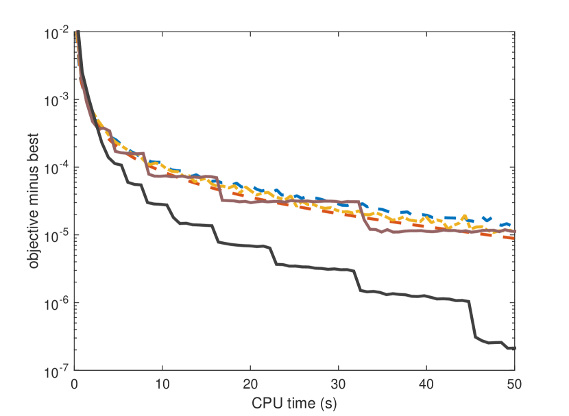
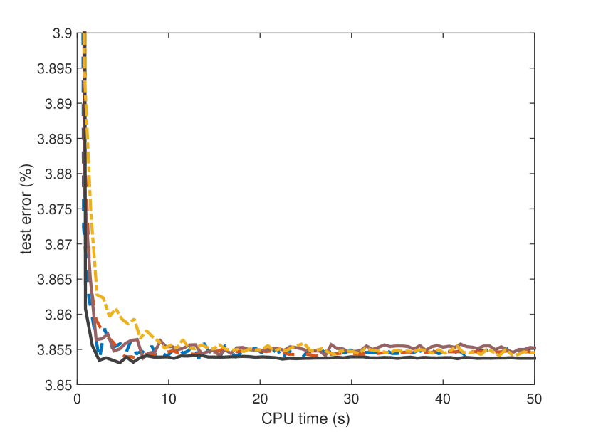
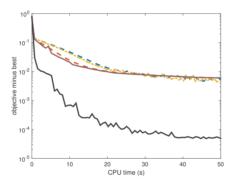
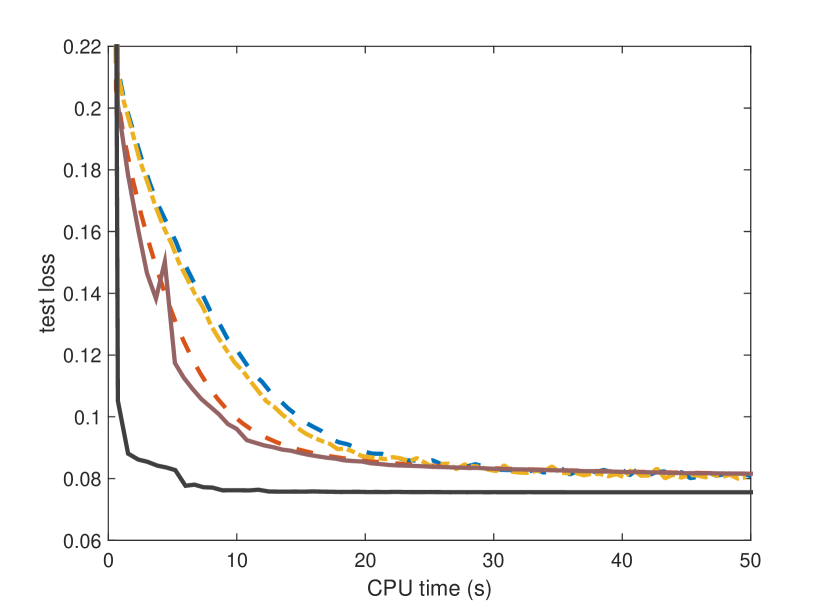
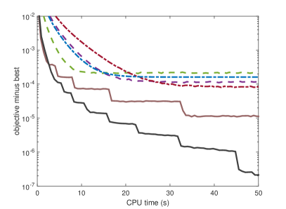
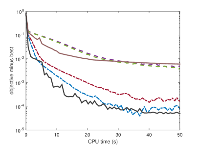
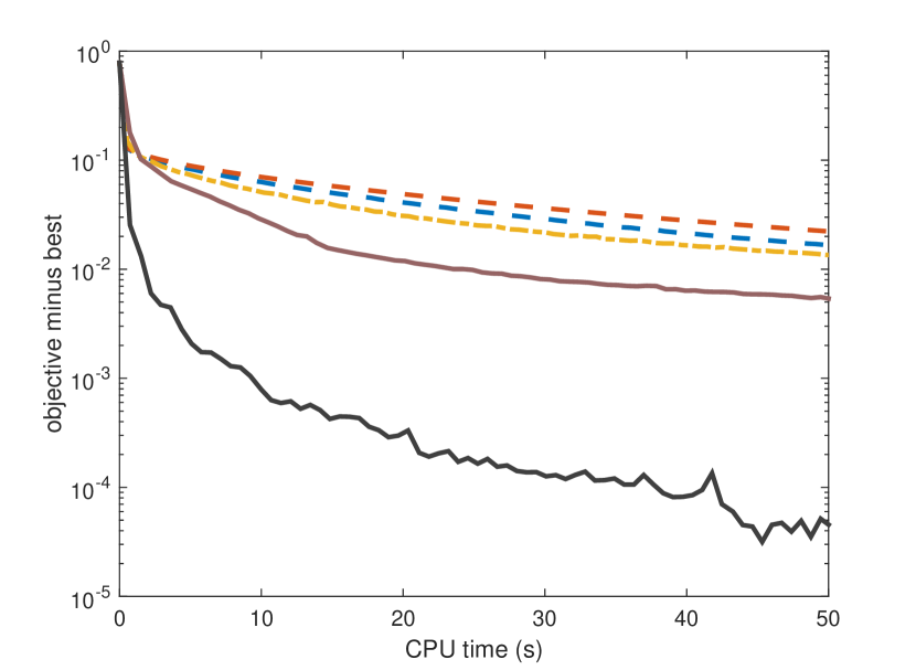
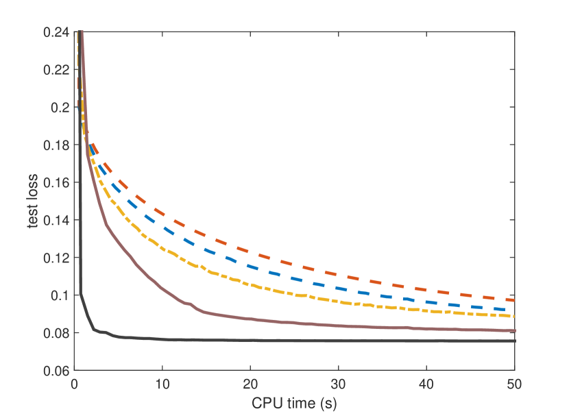
Figure 1 shows convergence of the objective and testing performance (classification error for rcv1 and $\ell_{1}$-loss for YearPredictionMSD). The trends are consistent with Theorem 1. CNS-A is the fastest (with a of $O(1/T^{2})$). This is followed by CNS-NA and Poly-SGD, both with $O(1/T)$ rate (from Theorem 1 and (?)). The slowest are FOBOS and RDA, which converge at a rate of $O(\log T/T)$ (?; ?).

rcv1.

YearPredictionMSD.

Figure 1: Objective (top) and testing performance (bottom) vs CPU time (in seconds) on a strongly convex problem.

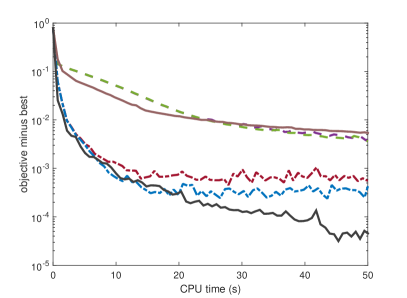
Figure 2 compares with the case where continuation is not used. Two fixed smoothness settings, $\gamma=10^{-2}$ and $\gamma=10^{-3}$, are used. As can be seen, they are much slower (Propositions 2 and 3). Moreover, a smaller $\gamma$ leads to slower convergence but better solution, while a larger $\gamma$ leads to faster convergence but worse solution. This is also consistent with Proposition 1, as using a fixed $\gamma$ only allows convergence to the optimal solution with a tolerance of $(1+\rho^{S})\gamma D_{u}$. Moreover, a smaller $\gamma$ leads to a larger condition number, and convergence becomes slower.

(a) rcv1.

(b) YearPredictionMSD.

Figure 2: Effect of continuation (strongly convex problem).

General Convex Objectives

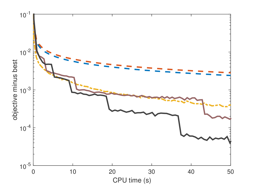
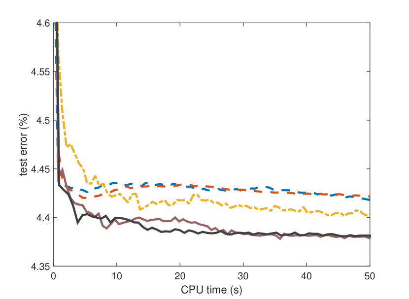
We set $\lambda_{1}$ in Algorithm 2 to $10^{-5}$ for rcv1, and $10^{-7}$ for YearPredictionMSD. As can be seen from Figure 3, the trends are again consistent with Theorem 3. CNS-A is the fastest ($O(1/T)$ convergence rate), while the others all have a rate of $O(1/\sqrt{T})$ (?; ?; ?). Also, RDA shows better performance than FOBOS and Poly-SGD. Recall that Poly-SGD outperforms FOBOS and RDA on strongly convex problems. However, on general convex problems, Poly-SGD is the worst as its rate is only as good as others, and it does not exploit the composite structure of the problem.

rcv1.

YearPredictionMSD.

Figure 3: Objective (top) and testing performance (bottom) vs CPU time (in seconds) on a general convex problem.

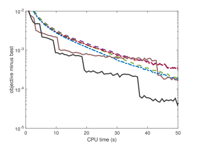
Figure 4 compares with the case where continuation is not used. As in the previous section, CNS-NA and CNS-A show faster convergence than its fixed-smoothing counterparts.

(a) rcv1.

(b) YearPredictionMSD.

Figure 4: Effect of continuation (general convex problem).

Conclusion

In this paper, we proposed a continuation algorithm (CNS) for regularized risk minimization problems, in which both the loss and regularizer may be nonsmooth. In each of its stages, the smoothed subproblem can be easily solved by either existing accelerated or non-accelerated solvers. Theoretical analysis establishes convergence results on the whole continuation algorithm, not just one of its stages. In particular, when accelerated solvers are used, the proposed CNS algorithm achieves the rate of $O(1/T^{2})$ on strongly convex problems, and $O(1/T)$ on general convex problems. These are the fastest known rates for nonsmooth optimization. However, CNS is advantageous in that it allows the use of a regularizer (unlike the fastest batch algorithm) and can exploit the composite structure of the optimization problem (unlike the fastest stochastic algorithm). Experiments on nonsmooth classification and regression models demonstrate that CNS outperforms the state-of-the-art.

References

- [Agarwal et al. 2009] Agarwal, A.; Wainwright, M. J.; Bartlett, P. L.; and Ravikumar, P. K. 2009. Information-theoretic lower bounds on the oracle complexity of convex optimization. In Advances in Neural Information Processing Systems, 1–9.
- [Becker, Bobin, and Candès 2011] Becker, S.; Bobin, J.; and Candès, E. J. 2011. NESTA: A fast and accurate first-order method for sparse recovery. SIAM Journal on Imaging Sciences 4(1):1–39.
- [Chen et al. 2012] Chen, X.; Lin, Q.; Kim, S.; Carbonell, J. G.; Xing, E. P.; et al. 2012. Smoothing proximal gradient method for general structured sparse regression. Annals of Applied Statistics 6(2):719–752.
- [Defazio, Bach, and Lacoste-Julien 2014] Defazio, A.; Bach, F.; and Lacoste-Julien, S. 2014. SAGA: A fast incremental gradient method with support for non-strongly convex composite objectives. In Advances in Neural Information Processing Systems, 2116–2124.
- [Duchi and Singer 2009] Duchi, J., and Singer, Y. 2009. Efficient online and batch learning using forward backward splitting. Journal of Machine Learning Research 10:2899–2934.
- [Hale, Yin, and Zhang 2007] Hale, E.; Yin, W.; and Zhang, Y. 2007. A fixed-point continuation method for -regularized minimization with applications to compressed sensing. Technical Report CAAM TR07-07, Rice University.
- [Johnson and Zhang 2013] Johnson, R., and Zhang, T. 2013. Accelerating stochastic gradient descent using predictive variance reduction. In Advances in Neural Information Processing Systems, 315–323.
- [Kushner and Yin 2003] Kushner, H. J., and Yin, G. 2003. Stochastic Approximation and Recursive Algorithms and Applications, volume 35. Springer Science & Business Media.
- [Mairal 2013] Mairal, J. 2013. Optimization with first-order surrogate functions. In Proceedings of the 30th International Conference on Machine Learning.
- [Mazumder, Hastie, and Tibshirani 2010] Mazumder, R.; Hastie, T.; and Tibshirani, R. 2010. Spectral regularization algorithms for learning large incomplete matrices. Journal of Machine Learning Research 11:2287–2322.
- [Nemirovski and Yudin 1983] Nemirovski, A., and Yudin, D. 1983. Problem Complexity and Method Efficiency in Optimization. Wiley.
- [Nesterov 2004] Nesterov, Y. 2004. Introductory Lectures on Convex Optimization, volume 87. Springer.
- [Nesterov 2005a] Nesterov, Y. 2005a. Excessive gap technique in nonsmooth convex minimization. SIAM Journal on Optimization 16(1):235–249.
- [Nesterov 2005b] Nesterov, Y. 2005b. Smooth minimization of non-smooth functions. Mathematical Programming 103(1):127–152.
- [Nesterov 2013] Nesterov, Y. 2013. Gradient methods for minimizing composite functions. Mathematical Programming 140(1):125–161.
- [Nitanda 2014] Nitanda, A. 2014. Stochastic proximal gradient descent with acceleration techniques. In Advances in Neural Information Processing Systems, 1574–1582.
- [Orabona, Argyriou, and Srebro 2012] Orabona, F.; Argyriou, A.; and Srebro, N. 2012. PRISMA: Proximal iterative smoothing algorithm. Preprint arXiv:1206.2372.
- [Ouyang and Gray 2012] Ouyang, H., and Gray, A. G. 2012. Stochastic smoothing for nonsmooth minimizations: Accelerating SGD by exploiting structure. In Proceedings of the 29th International Conference on Machine Learning, 33–40.
- [Parikh and Boyd 2014] Parikh, N., and Boyd, S. 2014. Proximal algorithms. Foundations and Trends in Optimization 1(3):127–239.
- [Rakhlin, Shamir, and Sridharan 2012] Rakhlin, A.; Shamir, O.; and Sridharan, K. 2012. Making gradient descent optimal for strongly convex stochastic optimization. In Proceedings of the 29th International Conference on Machine Learning, 449–456.
- [Schmidt, Roux, and Bach 2011] Schmidt, M.; Roux, N. L.; and Bach, F. R. 2011. Convergence rates of inexact proximal-gradient methods for convex optimization. In Advances in Neural Information Processing Systems, 1458–1466.
- [Schmidt, Roux, and Bach 2013] Schmidt, M.; Roux, N. L.; and Bach, F. 2013. Minimizing finite sums with the stochastic average gradient. Preprint arXiv:1309.2388.
- [Shalev-Shwartz and Zhang 2014] Shalev-Shwartz, S., and Zhang, T. 2014. Accelerated proximal stochastic dual coordinate ascent for regularized loss minimization. In Proceedings of the 31st International Conference on Machine Learning, 64–72.
- [Shamir and Zhang 2013] Shamir, O., and Zhang, T. 2013. Stochastic gradient descent for non-smooth optimization: Convergence results and optimal averaging schemes. In Proceedings of the 30th International Conference on Machine Learning, 71–79.
- [Wen et al. 2010] Wen, Z.; Yin, W.; Goldfarb, D.; and Zhang, Y. 2010. A fast algorithm for sparse reconstruction based on shrinkage, subspace optimization, and continuation. SIAM Journal on Scientific Computing 32(4):1832–1857.
- [Xiao and Zhang 2012] Xiao, L., and Zhang, T. 2012. A proximal-gradient homotopy method for the -regularized least-squares problem. In Proceedings of the 29th International Conference on Machine Learning, 839–846.
- [Xiao and Zhang 2014] Xiao, L., and Zhang, T. 2014. A proximal stochastic gradient method with progressive variance reduction. SIAM Journal on Optimization 24(4):2057–2075.
- [Xiao 2009] Xiao, L. 2009. Dual averaging method for regularized stochastic learning and online optimization. In Advances in Neural Information Processing Systems, 2116–2124.
- [Zou and Hastie 2005] Zou, H., and Hastie, T. 2005. Regularization and variable selection via the elastic net. Journal of the Royal Statistical Society: Series B 67(2):301–320.