Dependence of stellar magnetic activity cycles on rotational period in nonlinear solar-type dynamo

Abstract

We study turbulent generation of large-scale magnetic fields using nonlinear dynamo models for solar-type stars in the range of rotational periods from 14 to 30 days. Our models take into account non-linear effects of dynamical quenching of magnetic helicity, and escape of magnetic field from the dynamo region due to magnetic buoyancy. The results show that the observed correlation between the period of rotation and the duration of activity cycles can be explained in the framework of a distributed dynamo model with a dynamical magnetic feedback acting on the turbulent generation either from magnetic buoyancy or magnetic helicity. We discuss implications of our findings for the understanding of dynamo processes operating in solar-like stars.

1 Introduction

The solar-type cyclic magnetic activity is often observed among main-sequence stars with external convective envelopes (e.g., Baliunas et al., 1995; Hall et al., 2007). After Parker (1955), it is widely believed that the magnetic activity on solar-like stars results from large-scale dynamo processes driven by turbulent convection and rotation. Interpretation of the stellar magnetic activity is rather complicated because of nonlinear dynamo effects that needs to be taken into account (Noyes et al., 1984). Moreover, even in the case of the solar dynamo many details are poorly known (Charbonneau, 2011). In particular, the origin of the large-scale poloidal magnetic field of the Sun (the component of the field which lies in meridional planes) is not well understood.

One of the interesting question is how observations of stellar magnetic activity can help us in understanding the key processes of the solar dynamo and vice verse (Brun et al., 2014). The dependence of magnetic activity cycles on the period of rotation is of particular interest. Observations show that the stellar magnetic activity grows almost linearly with the increasing rotation rate (Vidotto et al., 2014), but the dynamo period decreases (Noyes et al., 1984). Thus, the solar-like stars show an anti-correlation between the dynamo period and the amplitude of magnetic activity. It is interesting that this relationship can be deduced from the solar activity data (Vitinsky et al., 1986), as well. A comparative study of this relation for solar and stellar cycles was published by Soon et al. (1994). Further studies revealed that this correlation is not unique, and that several branches corresponding to different magnetic activity levels can be identified (Saar & Brandenburg, 1999; Böhm-Vitense, 2007; Saar, 2011).

Theoretically, the observed correlation between the amplitude and period of the dynamo cycle is expected in a kinematic regime (Noyes et al., 1984). However, results of such linear analysis can not be applied to the nonlinear dynamo. Theoretical arguments of Noyes et al. (1984), and, also, Tobias (1998) and Ossendrijver (1997) had shown that dynamo saturation mechanisms affect the correlation. Also, the dynamo scenario type is important in this context. The concept of flux-transport dynamo has been popular in the solar community (Charbonneau, 2011). However, the stellar dynamo models which were constructed following this idea show a growth of the cycle period with an increase of the rotation rate, (e.g., see, Jouve et al. 2010, and Karak et al. 2014). This contradicts to the observations. The solution of this issue is not clear yet. Jouve et al. (2010) found that in the framework of the flux-transport models this issue can be resolved by assuming certain multiple-cell patterns of the meridional circulation. However, it is unclear how such circulation patterns are compatible with the angular momentum balance in stars. Pipin (2015) argued that the problem with the flux-transport models can be related to the direction of the dynamo wave propagation in the convective zone. In the flux-transport models the dynamo wave propagates inward from high to low latitudes towards the regions with low magnetic diffusivity. This causes an increase of the dynamo period when the large-scale toroidal field concentrates stronger at the bottom of the convection zone. Such effect has been found in 3D dynamo simulations by Guerrero et al (2016). In the distributed dynamo models (Brandenburg, 2005; Pipin & Kosovichev, 2011b) the dynamo wave propagates outwards from high to low latitudes. This type of dynamo agrees with observations in case both of the solar (Pipin & Kosovichev, 2011a; Pipin et al., 2012) and stellar cycles (Pipin, 2015).

In this paper we study the influence of nonlinear dynamo saturation mechanisms on basic properties of the magnetic activity cycles in solar-like stars with different rotation rates. We restrict ourselves by slowly rotating stars with the rotational periods from 14 to 30 days. In these cases the magnetic feedback on the differential rotation is not very strong compared to the saturation caused by magnetic buoyancy and magnetic helicity. From the results of Pipin (2015) it follows that the strongest variations of the latitudinal rotational shear due to the dynamo-generated magnetic activity are about 1% of the mean value for the case of a solar analog rotating with the period of 14 days. This agrees with the observational findings of Saar (2011), as well. The impact of such variations on the dynamo processes is not as strong as of the others nonlinear effects. Thus, we neglect variations of the differential rotation in this study.

2 Basic equations

2.1 Dynamo model

Following Krause & Rädler (1980), we explore the evolution of the induction vector of the mean magnetic field, $\overline{\mathbf{B}}$, in a highly conductive turbulent media with the mean flow velocity, $\overline{\mathbf{U}}$, and the mean electromotive force, $\boldsymbol{\mathcal{E}}=\overline{\mathbf{u}\times\mathbf{b}}$ (hereafter MEMF), where $\mathbf{u}$ and $\mathbf{b}$ are small-scale turbulent fluctuations of the flow velocity and magnetic field:

$$\frac{\partial\overline{\mathbf{B}}}{\partial t}=\boldsymbol{\nabla}\times\left(\boldsymbol{\mathcal{E}}+\overline{\mathbf{U}}\times\overline{\mathbf{B}}\right)\text{.}$$ (1)

We employ a decomposition of the axisymmetric field into a sum of the azimuthal (toroidal) and poloidal (meridional plane) components:

$$\overline{\mathbf{B}}=\mathbf{e}_{\phi}B+\nabla\times\frac{A\mathbf{e}_{\phi}}{r\sin\theta},$$

where $\mathbf{e}_{\phi}$ is the unit vector in the azimuthal direction, $\theta$ is the polar angle, and $A\mathbf{e}_{\phi}$ is the vector-potential of the large-scale poloidal magnetic field. The mean electromotive force, $\boldsymbol{\mathcal{E}}$, is expressed as follows:

$$\mathcal{E}_{i}=\left(\alpha_{ij}+\gamma_{ij}\right)\overline{B}_{j}-\eta_{ijk}\nabla_{j}\overline{B}_{k}.$$ (2)

The tensor, $\alpha_{ij}$, models the generation of the magnetic field by the $\alpha$ effect; the anti-symmetric tensor, $\gamma_{ij}$, controls pumping of the large-scale magnetic fields in the turbulent media; the tensor, $\eta_{ijk}$, governs the turbulent diffusion and takes into account the generation of the magnetic fields by the $\Omega\times J$ effect (Rädler, 1969). We take into account the effect of rotation and magnetic field on the mean-electromotive force. Here, we study of the dynamo saturation due to the nonlinear $\alpha$ effect and magnetic buoyancy.

The $\alpha$ effect takes into account the kinetic and magnetic helicities in the following form:

$$\alpha_{ij} = C_{\alpha}\sin^{2}\theta\psi_{\alpha}(\beta)\alpha_{ij}^{(H)}\eta_{T}+\alpha_{ij}^{(M)}\frac{\overline{\chi}\tau_{c}}{4\pi\overline{\rho}\ell^{2}}$$ (3)

where $C_{\alpha}$ is a free parameter, the $\alpha_{ij}^{(H)}$ and $\alpha_{ij}^{(M)}$ express the kinetic and magnetic helicity parts of the $\alpha$ effect, respectively; $\overline{\chi}$ is the small-scale magnetic helicity, $\ell$ is the typical length scale of the turbulence, and $\eta_{T}$ is the turbulent diffusivity. Tensors $\alpha_{ij}^{(H)}$ and $\alpha_{ij}^{(M)}$ depend on the Coriolis number, $\Omega^{*}=4\pi{\displaystyle\frac{\tau_{c}}{P_{rot}}}$, where $P_{rot}$ is the rotational period, $\tau_{c}$ is the convective turnover time. The reader can find a detailed description of these parameters in the paper of Pipin (2015). The magnetic quenching function of the hydrodynamical part of the $\alpha$ effect is defined as:

$$\psi_{\alpha}=\frac{5}{128\beta^{4}}\left(16\beta^{2}-3-3\left(4\beta^{2}-1\right)\frac{\arctan\left(2\beta\right)}{2\beta}\right),$$ (4)

where $\beta=\left|\mathbf{B}\right|/\sqrt{4\pi\overline{\rho}u^{\prime 2}}$, $u^{\prime}$ is the RMS of the convective velocity. This is so-called “algebraic” quenching describes the “instantaneous” magnetic feedback on the dynamo generation. It is assumed that the large-scale magnetic field varies much slower than the typical convective time-scale. In addition, there is a so-called “dynamical” quenching due to the magnetic helicity conservation (Pouquet et al., 1975). Similarly to Kleeorin & Ruzmaikin (1982), Blackman & Brandenburg (2003) and Kleeorin et al. (2003) (also, see, Kitiashvili & Kosovichev 2009; Sokoloff et al. 2013; Blackman & Subramanian 2013), we model this effect though the second term of Eq.(3) and the equation which governs the evolution of the helicity density of the fluctuating part of magnetic field, $\overline{\chi}$, (Hubbard & Brandenburg, 2012; Pipin et al., 2013):

$$\frac{\partial\overline{\chi}^{(tot)}}{\partial t}=-\frac{\overline{\chi}}{R_{m}\tau_{c}}-2\eta\overline{\mathbf{B}}\cdot\mathbf{\overline{J}}-\boldsymbol{\nabla\cdot}\boldsymbol{\boldsymbol{\mathcal{F}}}^{\chi},$$ (5)

where $\overline{\chi}^{(tot)}=\overline{\chi}+\overline{\mathbf{A}}\cdot\overline{\mathbf{B}}$ is the total magnetic helicity density, and the $\boldsymbol{\boldsymbol{\mathcal{F}}}^{\chi}$ is the diffusive flux of the magnetic helicity, $R_{m}$ is the magnetic Reynolds number, and $\eta$ is the microscopic magnetic diffusivity.

The turbulent mean-field pumping contains a sum of contributions due to the mean density gradient (Kichatinov, 1991), $\gamma_{ij}^{(\rho)}$, the diamagnetic pumping (Krivodubskij, 1987), $\gamma_{ij}^{(\eta)}$, the mean-field magnetic buoyancy (Kichatinov & Pipin, 1993), $\gamma_{ij}^{(b)}$, and due to effects of the large-scale shear (Pipin, 2013), $\gamma_{ij}^{(H)}$:

$$\gamma_{ij}=\gamma_{ij}^{(\rho)}+\gamma_{ij}^{(\eta)}+\gamma_{ij}^{(b)}+\gamma_{ij}^{(H)}.$$ (6)

In our study the most essential pumping is related to the mean-field magnetic buoyancy:

$$\gamma_{ij}^{(b)} = \frac{\alpha_{MLT}u^{\prime}}{\gamma}\beta^{2}K\left(\beta\right)g_{n}\varepsilon_{inj},$$

where $\alpha_{MLT}$ is the mixing-length parameter, $\gamma$ is the adiabatic exponent, and $\mathbf{g}$ is the unit vector in the radial direction. The quenching of the magnetic buoyancy (see Kichatinov & Pipin 1993) is defined by function $K\left(\beta\right)$:

$$K\left(\beta\right)=\frac{1}{16\beta^{4}}\left(\frac{\left(\beta^{2}-3\right)}{\beta}\arctan\left(\beta\right)+\frac{\left(\beta^{2}+3\right)}{\left(\beta^{2}+1\right)}\right).$$

A detailed formulation has been published by Pipin (2015). The distribution of the turbulent parameters, e.g, such as the typical convective turn-over time, $\tau_{c}$, the mixing length, $\ell$, the RMS convective velocity, $u^{\prime}$, the mean density, $\bar{\rho}$ and its gradient $\mathbf{\boldsymbol{\Lambda}}^{(\rho)}=\boldsymbol{\nabla}\log\overline{\rho}$ are computed using the mixing-length model of the solar convection zone of Stix (2002). In particular, it uses the mixing length $\ell=\alpha_{{\rm MLT}}\left|\Lambda^{(p)}\right|^{-1}$, where $\Lambda{}^{(p)}={\nabla}\log\overline{p}$, is the inverse pressure height, and $\alpha_{{\rm MLT}}=2$. The turbulent diffusivity profile is given in the form $\eta_{T}=C_{\eta}{\displaystyle\frac{u^{\prime 2}\tau_{c}}{3f_{ov}\left(r\right)}}$, where function $f_{ov}(r)=1+\exp\left(50\left(r_{ov}-r\right)\right)$, controls quenching of the turbulent effects near the bottom of the convection zone, $r_{ov}=0.725R_{\odot}$ . The parameter $C_{\eta}$, (in the range $0<C_{\eta}<1$) is a free parameter that controls the efficiency of large-scale magnetic field mixing by turbulence. It is used to adjust the period of the dynamo cycle. We use the same model of the convection zone for all the rotational periods considered in this paper.

At the bottom of the convection zone we apply a perfectly conducting boundary condition. At the top of the convection zone the poloidal field is smoothly matched to the external potential field, and the toroidal field is allowed to penetrated to the surface:

$$\delta\frac{\eta_{T}}{r_{e}}B+\left(1-\delta\right)\mathcal{E}_{\theta} = 0,$$ (7)

where $\delta=0.99$ (Moss & Brandenburg, 1992; Pipin & Kosovichev, 2011b). The numerical integration is carried out in latitude from the pole to pole, and in radius, from $r_{b}=0.715R_{\odot}$ to $r_{e}=0.99R_{\odot}$. The numerical scheme employs the pseudo-spectral approach for the numerical integration in latitude and the second-order finite differences in radius.

Runs	Quenching	Dynamo Period, [YR]	Flux, 1024[MX]	$\overline{\left|B^{\left(p\right)}\right|}$, [G]	Polar, $\left|B_{r}\right|$, [G]
M0	AQ	13.2, 14, 17.6, 21, 21.4, 23	2.2, 6.4, 11.4, 14.8, 18.3, 20.8	10, 12, 15, 23, 25, 27	11, 20, 25, 29, 30, 31
M1	AQ, BQ	11.1, 8.8, 6.8, 5, 4.8, 4.6	0.7, 1.2, 1.5, 1.7, 1.8, 1.9	3, 5.5, 8, 10, 7.5, 6.8	2, 4, 4.3, 3.8, 3.6, 3.4
M2 , $R_{m}=10^{6}$	MHQ	12.7, 10.8, 8.1, 6.6, 6.2, 5.2(5.9)	0.4, 1., 1.9, 2.7, 3, 3.6	1.5, 2.7, 3.1, 3.1, 4.3, 7.5	1.5, 2.5, 2., 3.5, 2.8, 7.8
M3	MHQ, BQ ,AQ	11.6, 9.9,7.2, 5.8, 5.4, 5	0.4, 0.9, 1.3, 1.8, 1.9, 2.1	2.3, 2.5, 3.4, 3.1, 4.5, 7	2.2, 2.3, 1.9, 2.5, 3.2, 4
M3A, $C_{\alpha}=0.03$	-/-	12.4, 11, 8.4, 6.5, 6.1, 5.5	0.3, 0.6, 1.1, 1.5, 1.7, 1.9	1.3, 2.4, 3.2, 3.5, 3.6, 4.5	1.3, 2.1, 1.7, 1.7, 2.1, 2.7
M3B, $C_{\alpha}=0.06$	-/-	9.5, 7.6, 5.7, 4.7, 4.5, 4.0	0.8, 1.3, 1.9, 2.3, 2.5, 2.8	3.9, 4.7, 7.2, 11.3, 13.7, 16	3.2, 2.9, 4.6, 20, 28, 44

Table 1: Results of the model runs for the set of six rotational periods $P_{rot}=\left[29.4,25,20,16.7,15.6,14.3\right]$ days from left to right in each cell. Four types of the dynamo models with different non-linear quenching mechanisms (second column): the algebraic quenching (AQ), the magnetic buoyancy quenching (BQ) and, the magnetic helicity quenching (MHQ). The other columns show the dynamo period, the total unsigned magnetic flux, the mean poloidal magnetic field strength at the surface, $\overline{\left|B^{\left(p\right)}\right|}$, the strength of the radial polar field, $\left|B_{r}\right|$ .

3 Results

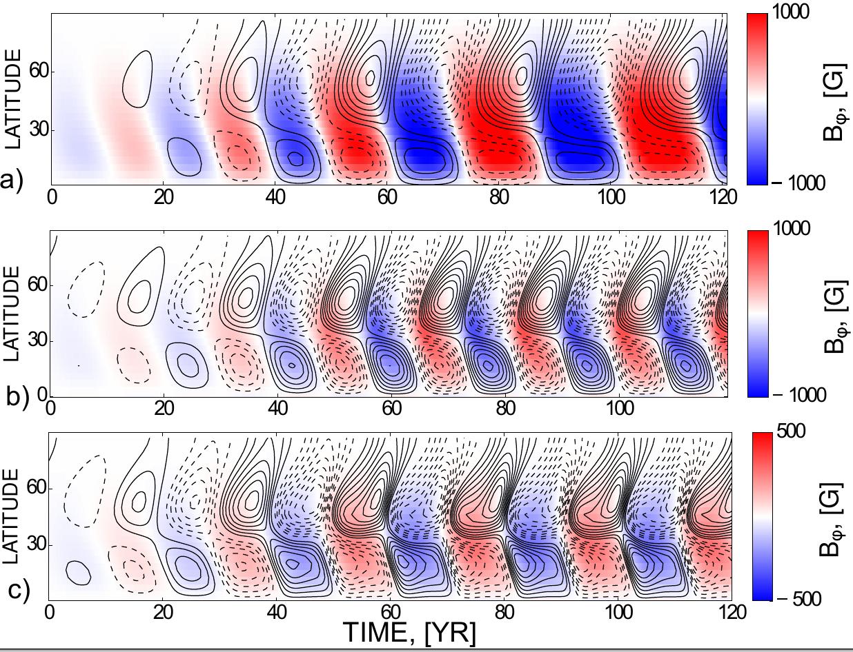
Figure 1: Time-latitude diagrams for the radial magnetic field at the surface (contours) and the toroidal field in the subsurface layer (background image) for the rotational period of 25 days: a) model M0; b) model M1; c) model M2 (Table 1). The strength of the radial field varies in range of $\pm$20G in model M0, $\pm 5$G in model M1 and $\pm 3$G in model M2.

The free parameters, $C_{\alpha}$, $C_{\eta}$ and $R_{m}$ are used to calibrate the model for the best possible agreement with the solar-cycle observations for the solar rotation period. In this study we use $C_{\alpha}=0.04$, $C_{\eta}=0.05$ and $R_{m}=10^{4}$. In model M2 (Table 1) we use $R_{m}=10^{6}$, which provides a better conservation of magnetic helicity, which is the primary non-linear effect in this case. The profile of the rotation law is taken from the helioseismology inversion of Howe et al. (2011). It is fixed, as well (see, Pipin 2015). However, the radial profile of the Coriolis number $\Omega^{*}=4\pi{\displaystyle\frac{\tau_{c}}{P_{rot}}}$ varies with the rotational period. In our runs, we employ the following set of rotational periods:

$$P_{rot}=\left[29.4,25,20,16.7,15.6,14.3\right]$$ (8)

For this set we compute the dynamo models (Eqs(1,5)) taking into account the different saturation mechanisms, as specified in Table 1. The models which are listed in Table 1 employ the $\alpha$ effect parameter, $C_{\alpha}=0.04$. This value is of twenty percents above the threshold for the $P_{rot}=25$ days. Table 1 also shows results for the dynamo cycle period, the magnitude of the unsigned magnetic flux generated in the whole convection zone, the mean strength of the poloidal magnetic field at the surface, $\overline{\left|B^{\left(p\right)}\right|}$ , (which we will use as a proxy of the line-of-sight magnetic field strength), and the strength of the radial polar magnetic field, $\left|B_{r}\right|$, during the cycle minimum. The dynamo models are calculated untill they reach a stationary phase. In the study we consider the magnetic field geometry antisymmetric relative to the equator. This is done via imposing a weak seed poloidal magnetic field of the dipole symmetry in the initial conditions. Model M3 was explored for a set of the $\alpha$ effect parameter, $C_{\alpha}=[0.03,0.04,0.06]$. Also, for model M2 we made additional runs for the rotational periods 16.7 and 15.6 days using $C_{\alpha}=0.06$ and $C_{\alpha}=0.05$ respectively to study the behavior of the long-term variations in the dynamo process for different rotational periods.

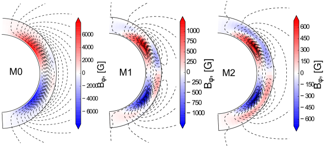
Figure 2: Snapshots of magnetic field distributions in the minimum of the magnetic cycle for models M0, M1 and M2 (Table 1) for the samerotational period 25 day, the color background image shows the strength of the toroidal magnetic field and contours show streamlines of the poloidal magnetic field. The strength of the poloidal field is given in Table 1.

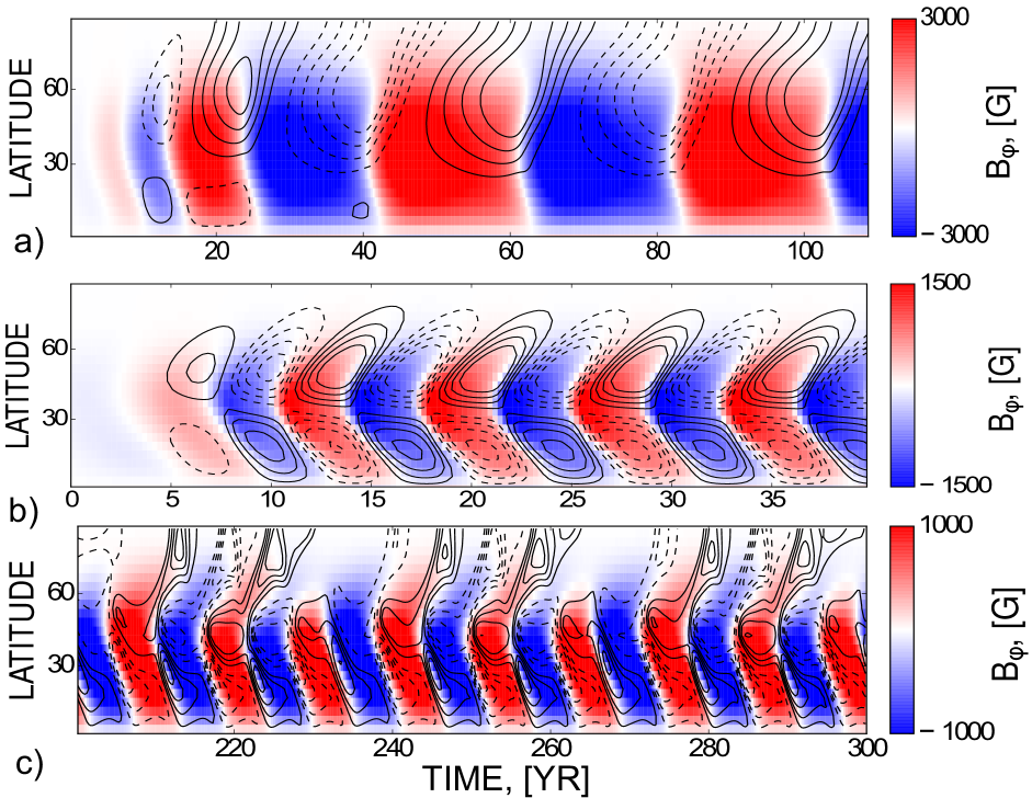
Figure 3: The same as Fig.1 for the rotational period 14 days. Model M2 has a much longer relaxation time. The radial magnetic field varies in range $\pm 25$G in model M0, $\pm 5$G in M1 and $\pm 15$G in M2.

The effect of the quenching mechanisms on the time-latitude evolution of the toroidal and poloidal magnetic field is illustrated in Figures 1, 2 and 3, where we show results for the rotational periods of 25 and 16.7 days for models M0, M1 and M2. For the rotation period of 25 days all models produce the solar-like time-latitude magnetic butterfly diagrams. Model M0 has the strongest large-scale magnetic field, and it has the longest dynamo period among all the runs (see Table 1). It is also seen that the dynamo period in model M0 increases when the dynamo approaches the stationary state. This seems to be due to the strong concentration of the dynamo wave near the bottom of the convection zone in model M0. This is illustrated by snapshots of the magnetic fields distributions in Figure 2.

Increasing the rotation rate results in an increase of the dynamo period in model M0 because the toroidal field is amplified near the bottom of the convection zone. Simultaneously, the $\alpha$ effect is suppressed there. This results in a spatial separation of the dynamo generation by the $\alpha$ and $\Omega$ effects. Deinzer et al. (1974) had shown that this causes an increase of the dynamo period. Note, that in the flux-transport models the $\alpha$ and $\Omega$ effects are spatially separated by design of the models. Models M1, M2 and M3 show a decrease of the dynamo period when the period of rotation decreases, as they preserve a distributed character of the dynamo process.

Increasing non-linearity in the dynamo process can increase the complexity of the dynamo evolution. This happens in model M2 for the rotational period of 14 days. The model shows a long-term modulation with a period of about 40 years while having two primary dynamo periods of 5.3 and 5.9 years. The modulation disappears when the kinetic helicity parameter $C_{\alpha}$ increases. Similar long-term modulations were found for the rotational periods 16.7 and 15.6 days with $C_{\alpha}=0.06$ and $C_{\alpha}=0.05$ respectively. The long-term modulation in axisymmetric dynamo models with the dynamical quenching of the $\alpha$ effect was demonstrated earlier in the number of papers (see, e.g., Covas et al. 1998; Kitiashvili & Kosovichev 2009). Model M2 illustrates an interesting possibility when the surface radial magnetic field almost disappears during the maximum of the grand cycle of the toroidal magnetic field. A situation when the toroidal field dominates on the stellar surface is also observed in stellar activity, but for a non-axisymmetric field, and for the faster rotating star, see, e.g., the review by Donati & Landstreet (2009).

Variations of the total unsigned flux of the toroidal field in the convection zone for the star rotating with the period of 16 days are shown in Figure 4. It is seen that the non-linear mechanism involved in the dynamo affects the amplitude of the dynamo generated flux, the range and period of the variations. Model M2 has a long-term modulation of the magnetic activity for $C_{\alpha}=0.06$. The same effect is found for model M2 with the rotational period of 14 days and $C_{\alpha}=0.04$ (see Figure 3c). It is interesting that individual cycles are not always well recognized in the long-term modulations of the flux.

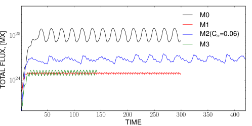
Figure 4: Variations of the total unsigned flux of toroidal field in the convection zone for the star rotating with period of 16 days. Model M2 has long-term modulation of the magnetic activity for $C_{\alpha}=0.06$.

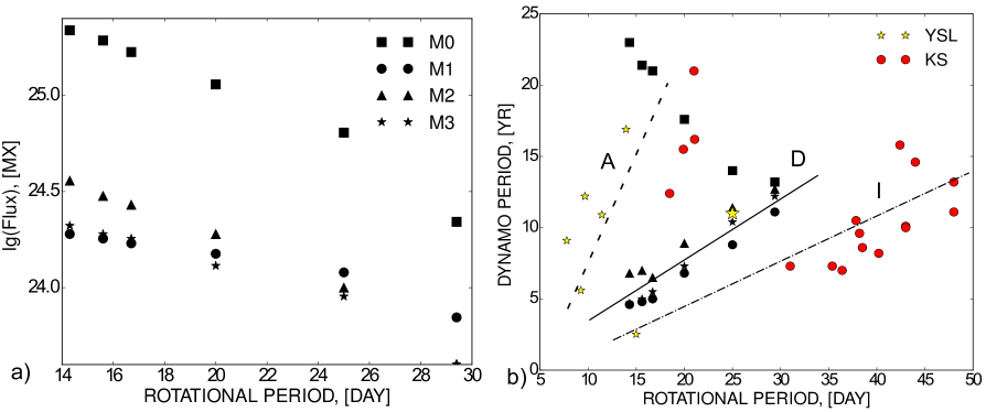
Figure 5: a) Dependence of the amplitude of dynamo generated magnetic flux in the convection zone on the period of rotation; b) the dynamo period vs the rotational period in the models (Table 1) and in sample of young solar like stars, denoted as YSL (the sample of G-stars from Böhm-Vitense, 2007), KS denotes the sample of K-stars from the same paper, the Sun is marked by big yellow symbol star. The “A” (dashed line) stands for the active branch, “I” (dash-dot line) - the inactive one and “D” (solid line) - the branch produced by our models M1 and M2.

Figure 5a shows the dependence of the dynamo generated unsigned magnetic flux in the convection zone on the period of rotation. It shows an increase of the generated flux with an increase of the rotation rate. It is seen that the magnetic helicity conservation produces the strongest quenching of the dynamo process among all the non-linear mechanisms.

Thus, variations of the dynamo period with the rotational period depend on the dynamo saturation mechanism. Figure 4b illustrates our results together with the observational results shown earlier by Böhm-Vitense (2007). The algebraic quenching of the $\alpha$ effect is a simple anzatz most widely used in various dynamo models. However, this non-linear effect results in an increase of the dynamo period with increasing rotation rate. This tendency disagrees with the observations. The opposite trend is demonstrated by models M1, M2 and M3. It qualitatively agrees with the observations that show a complicated behavior of the stellar activity periods, indicating the existence of two populations of magnetically “active” and “inactive” stars (Saar & Brandenburg, 1999; Böhm-Vitense, 2007; Saar, 2011).

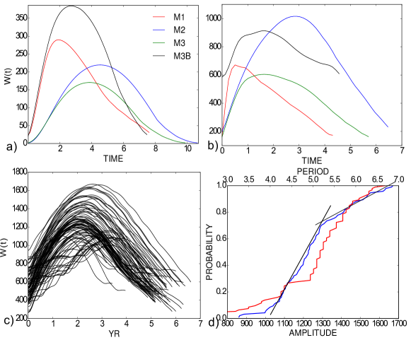
Figure 6: The Wolf number for the individual cycles: a) the rotational period of 25 days; b) the same for the rotational periods of 16 days; c) the set of cycles for the model M2 with long-term modulation, the rotational period 16 days and $C_{\alpha}=0.06$; d) Probability of the cycle amplitude(blue) and period (red) in the long-term modulation of magnetic activity. Two intervals with the different uniform probability distributions of the cycle amplitude are marked by the linear trends.

It is interesting to estimate how the magnetic activity changes parameters of spotness during the magnetic cycle. For this purpose we employ a simple relation between the Wolf susnspot number $W\left(t\right)$ and the amplitude of the toroidal magnetic field in the subsurface layer $B_{max}$,

$$W={\displaystyle B_{max}\exp\left(-\frac{B_{0}}{B_{max}}\right)},$$ (9)

where $B_{0}=1000$G (Pipin et al., 2012). The parameter $B_{0}$ is slightly different to that one used in the above cited paper, because here the $B_{max}$ value is estimated from the layer in the upper convection zone where the maximum of the dynamo wave is located. Thus, the depth of the $B_{max}$ is not fixed and it varies with time. This provides a smoother profile of $W(t)$ for the fast rotating stars compared to the previous definition. Examples of the Wolf number profiles for different models are shown in Figure 6. The cycle of the model M0 is substantially larger than in other models and it is not shown. It is seen that magnetic buoyancy is responsible for the most asymmetric profile of $W\left(t\right)$. Also, it is found that the rise time decreases when the cycle amplitude increases. This effect works in both cases for the decrease of the rotational period and for the increase of the $\alpha$-effect amplitude. Similar phenomenon is observed in solar activity (Vitinsky et al., 1986).

All models listed in Table 1, except model M2 with the rotational period 14 days, reach a stationary state, which is characterized by a non-linear oscillation of some fixed period. For the rotational periods of 14, 15, and 16 days we find long-term modulations in model M2 with $C_{\alpha}=\left[0.04,0.05,0.06\right]$ respectively. In these cases the basic dynamo period has no fixed value. For each time series of the theoretical Wolf number parameter $W$, we extract the individual cycles and compute the cycle parameters, i.e., the magnitude of the maximum, the period, the rise time and the decay time. We do this in the same way as previously in Pipin & Kosovichev (2011a). Figure 6c shows variations of $W$ for the individual cycle profiles. These profiles were extracted from the time series of model M2 with the rotational periods of 16 days, and $C_{\alpha}=0.06$. It is seen that the stronger cycles have longer period in this set. The amplitude of the period variations is about 3 years. The amplitude of $W$ varies about twice of the minimal amplitude. The probability distribution functions are constructed as follows. We sort the amplitudes of $W$ in the increasing order and compute the cumulative probability distribution:

$$CDF=\frac{\sum_{k=1}^{i}k}{N},$$ (10)

where, $i$ is the order number (after sorting the set in the increasing order), and $N$ is the total number of instances. In the set shown in Figure 6c $N=92$. Equation (10) approximates the probability for the amplitude of $W$ to have values in the interval between $W_{min}$ and $W_{i}$. The accuracy of the approximation improves as $N\rightarrow\infty$. The same procedure was repeated for the period parameter. The result is shown in Figure 6d (red curve). From this analysis we conclude that the amplitude of $W$ demonstrates the existence of two populations of the stellar cycles, which can be quantified as the “strong” and “weak” cycles. The two populations are not well recognized from the distribution of the dynamo period. Other examples of application of Eq(10) to analysis of the dynamo cycles were presented by Pipin & Sokoloff (2011).

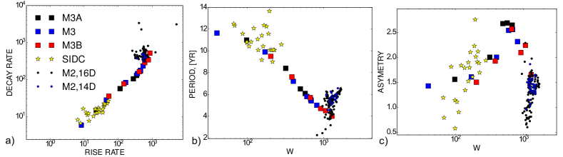
Figure 7: Theoretical Waldmeier’s relations in stellar cycles. The “SIDC” is related to the sunspot database (SIDC, 2010)

It is interesting to look how the Waldmeier relations, well-known for the sunspot cycles, and the asymmetry of stellar cycles can change with the rotational period, and the magnitude of the $\alpha$ effect. For this we consider model M2 and M3. For model M2 we use only runs with the long-term modulations. Similarly to Pipin & Kosovichev (2011a) we determine the mean rise and decay rate for each individual cycle in each simulatied time series of $W$. The asymmetry is determined as a ratio between the decay and rise rates. Figure 7 shows our results. Firstly, it is seen that this ratio seems to be constant for the set of the periodic dynamo models (without long-term modulations). The decay rates of the dynamo cycles vary consistently with the rise rate, with the increase of the alpha effect parameter $C_{\alpha}$ and the rotation rate. The theoretical trend is consistent with observations of the solar activity cycles. Here we used the data set provided by SIDC (2010). However, the time series for model M2 for the rotational periods of 14 and 16 days, which has the long-term modulation of the magnetic cycle are out of the trend. Figure 7b shows that these models have a correlation between the cycle amplitude and its period. That contradicts to the general trend of the periodic models and the solar observations as well. It is interesting to note that populations of the weak cycles in the long-term modulations follows the anti-correlation between the amplitude and period of cycle. The effect is not well recognized in Fig.7b because the scatter of the cycle parameters is relatively small. We find that this scatter is decreased with the increasing rotation rate. Also The periodic models show that asymmetry increases with the increase of the cycle magnitude (Fig.7c). The trend changes in stars with the high rotation rate and strong$\alpha$-effect. This is likely because our parameterization of the cycle asymmetry is too simple and it does not take into account the possible complicated form of $W$. For example, Fig.6b shows the profile of $W$ , in which a sharp rise of activity ends by a plateau, and the maximum is not well defined. The same arguments should be taken into account in analysis of the sunspot cycles. The models with the nonlinear long-term modulations do not show a dependence of the asymmetry on the cycle magnitude.

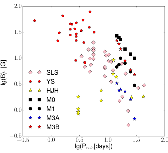
Figure 8: Comparison of our dynamo models with results of survey of Vidotto et al. (2014): the mean line-of-sight magnetic field on the surface vs the period of rotation, the SLS symbols show the solar-like stars, the YS - the young Suns, the HJH - stars host of hot Jupiters, notations of the model results are the same as in Figure 4.

Figure 5 shows a comparison of our dynamo models with the results of survey of Vidotto et al. (2014) for the absolute value of the mean line-of-sight magnetic field on the surface versus the period of rotation. We see that all the models qualitatively agree with the results of observations within the investigated range of the rotational periods. Model M0 shows a stronger magnetic field than it is found in the observations. This indicates on the presence of additional dynamo saturation mechanisms, like those implemented in models M1 and M2, i.e., the nonlinear quenching due to the magnetic buoyancy or the magnetic helicity. As noted in Introduction, for rapidly rotating stars the magnetic feedback on the differential rotation and convection has to be taken into account as well. Models M3A and M3B show different results for the different magnitude of the $\alpha$-effect parameter, $C_{\alpha}$. We see that the observed scatter of the magnetic field strength can be explained by variations of $C_{\alpha}$, varing by a factor of two above the dynamo instability threshold. From the solar dynamo models results we know that a similar effect can be produced by a small fluctuations of $\alpha$ on the time scale comparable with the length of the magnetic cycle (Moss et al., 2008).

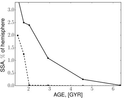
Figure 9: The theoretical sunspot area calculated for model M2, solid line shows the maximum value and the dashed line shows the minimum.

The investigated sample of rotational periods can be related to different ages of the sun-like stars. Taking into account the slowdown of rotation with time as $t^{-1/2}$, where $t$ is the star’s age (Skumanich, 1972), we deduce that age of stars in our sample can be found from the relation: ${\displaystyle t_{*}=t_{\odot}\left(\frac{P_{*}}{P_{\odot}}\right)^{2}}$ , where $P_{\odot}=25$ days and $t_{\odot}=4.61$ Gyr are parameters of the modern Sun. Thus, the investigated sample of the rotational periods covers the range of ages from 1.5 to 6.2 Gyr. However, on this time scale changes of the convection zone structure have to be taken into account. The percentage of disk occupied by sunspots is estimated from the empirical correlation $SSA\approx 16.7W/10^{4}$ (Vitinsky et al., 1986). Figure 6 shows our estimation for amplitude of $SSA$ at the maximum and minimum (dashed curve) of magnetic cycle with the age for model M2. It shows that the younger stars are significantly more spotty, This is a rather naive estimate which does not take into account mechanisms of the sunspot formations, and also changes of the convection zone and the differential rotation with the stellar age.

4 Discussion and conclusions

We have studied the nonlinear magnetic feedback on the turbulent generation of the large-scale magnetic fields by a solar-type dynamo for the range of rotation periods from 14 to 30 days. Our models take into account the non-linear $\alpha$ effect, the balance of magnetic helicity density, and escape of magnetic field from the dynamo region due to magnetic buoyancy. We did not consider the possible magnetic feedback on the differential rotation and changes in the convection zone stucture.

Currently, one of the most important observational tests for dynamo models of solar-like stars is the relationship between the magnetic cycle periods and the period of stellar rotation. Earlier, Noyes et al. (1984), also Ossendrijver (1997) and Tobias (1998) had suggested that despite a seemingly linear character of the connection between the rotational period and the dynamo period in stellar magnetic activity, the relation is not trivial because the large-scale dynamo goes to a non-linear regime when the rotation rate increases. The revealed multiple populations of magnetic activity in late-type stars (Saar & Brandenburg, 1999) showed that the theoretical interpretation of stellar magnetic activity can be complicated. It was suggested that the “active” population of stars operates the dynamo concentrated near the bottom of the convection zone, and the “inactive” population that operates (Saar & Brandenburg, 1999; Böhm-Vitense, 2007) a distributed dynamo. In most cases, the models of the first type show an increase of the dynamo period with increasing of rotation rate (Jouve et al., 2010; Karak et al., 2014; Pipin, 2015) and are not consistent with observations. Our results show that the observed correlation between the period of rotation and the dynamo period can be explained by the distributed dynamo models that includes the dynamical magnetic feedback on the turbulent generation either due to the magnetic buoyancy or the magnetic helicity. Note that the magnetic buoyancy effect which is employed in the paper is related to buoyancy of large-scale magnetic fields and not to the so-called flux-tube buoyancy (Parker, 1979). Kichatinov & Pipin (1993) discussed the issue in details.

In our set of dynamo models we did not find a satisfactory explanation of the observed multiple populations in terms of the stellar activity cycles periods. A number of possibile hypothesises remains to be explored. For example, our study is limited to magnetic field configurations that are anti-symmetric relative to the equator. The magnetic parity breaking is often considered as a source of non-linear long-term modulations of solar activity (Ivanova & Ruzmaikin, 1976; Brandenburg et al., 1989; Sokoloff & Nesme-Ribes, 1994; Weiss & Tobias, 2016). This may be the case for the stellar activity as well. The correlation between the period of rotation and the dynamo period could be affected by changes of the convection zone characteristics and changes of the differential rotation profile (Kitchatinov, 2011). Models with long-term modulations and dynamical quenching of the $\alpha$-effect by the magnetic helicity conservation show two populations of the activity cycles. The population of the weak cycles tends to follow standard the Waldmeir’s rules. But these do not hold for the whole time series.

Donati & Landstreet (2009) presentented a diagram of stellar magnetic activity for the period of rotation versus the stellar mass diagram of magnetic activity, which shows that fast rotating solar mass stars have non-axisymmetric magnetic fields. It is not clear if the non-axisymmetric field on the fast rotating solar analogs is generated by the dynamo instability or results from emergence of magnetic field on the surface. The non-axisymmetric fields is rarely discussed in the solar type dynamo. It presumes that the differential rotation suppresses the non-axisymmetric dynamo (Raedler, 1986). However, for the $\alpha\Omega$ dynamos, the critical threshold for generation of non-axisymmetric magnetic fields is only about a factor 2 or 3 larger than those for the axisymmetric dynamo. The interaction of the axisymmetric and non-axisymmetric modes was never studied for the super-critical regimes which could be operated in fast rotating stars. Finite non-axisymmetric perturbations can also affect the axisymmetric dynamo (Pipin & Kosovichev, 2015). Future studies should show if the observed multiple populations of magnetic cycles in stellar activity can be explored by differences between the axisymmetric and non-axisymmetric dynamo models.

VVP is supported by RFBR grant and the project II.16.3.1 of ISTP SB RAS. AGK is partially supported by NASA grant NNX14A070G

References

- Baliunas et al. (1995) Baliunas, S. L., et al. 1995, ApJ, 438, 269
- Blackman & Brandenburg (2003) Blackman, E. G., & Brandenburg, A. 2003, ApJ, 584, L99
- Blackman & Subramanian (2013) Blackman, E. G., & Subramanian, K. 2013, MNRAS, 429, 1398
- Böhm-Vitense (2007) Böhm-Vitense, E. 2007, ApJ, 657, 486
- Brandenburg (2005) Brandenburg, A. 2005, ApJ, 625, 539
- Brandenburg et al. (1989) Brandenburg, A., Krause, F., Meinel, R., Moss, D., & Tuominen, I. 1989, A&A, 213, 411
- Brun et al. (2014) Brun, A., Garcia, R., Houdek, G., Nandy, D., & Pinsonneault, M. 2014, Space Science Reviews, 1
- Charbonneau (2011) Charbonneau, P. 2011, Living Reviews in Solar Physics, 2, 2
- Covas et al. (1998) Covas, E., Tavakol, R., Tworkowski, A., & Brandenburg, A. 1998, A&A, 329, 350
- Deinzer et al. (1974) Deinzer, W., von Kusserow, H.-U., & Stix, M. 1974, A&A, 36, 69