Investigating multi-channel quantum tunneling in heavy-ion fusion reactions with Bayesian spectral deconvolution

Abstract

Excitations of colliding nuclei during a nuclear reaction considerably affect fusion cross sections at energies around the Coulomb barrier. It has been demonstrated that such channel coupling effects can be represented in terms of a distribution of multiple fusion barriers. I here apply a Bayesian approach to analyze the so called fusion barrier distributions. This method determines simultaneously the barrier parameters and the number of barriers. I particularly investigate the ¹⁶O+¹⁴⁴Sm and ¹⁶O+¹⁵⁴Sm systems in order to demonstrate the effectiveness of the method. The present analysis indicates that the fusion barrier distribution for the former system is most consistent with three fusion barriers, even though the experimental data show only two distinct peaks.

Quantum tunneling plays an important role in many areas of physics and chemistry. One good example is a nuclear fusion reaction in stars, which is responsible for stellar energy production and nucleosynthesis Adelberger98 . While one considers a penetration of a one-dimensional barrier in many applications, it is important to notice that in reality quantum tunneling often involves many degrees of freedom Caldeira81 and/or takes place in a multi-dimensional space TN94 ; SBDN09 . It is naturally expected that this results in a significant modification in tunneling rates.

In nuclear physics, a heavy-ion fusion reaction at energies around the Coulomb barrier is a typical example of quantum tunneling with many degrees of freedom BT98 ; HT12 . In order for fusion reactions to take place, the Coulomb barrier between the colliding nuclei has to be overcome, and thus the fusion reactions occur by quantum tunneling at low energies. Moreover, atomic nuclei are composite particles, and their internal degrees of freedom can be excited during fusion. It has been well recognized by now that such excitations lead to a large enhancement of fusion cross sections at subbarrier energies as compared to a prediction of a simple one-dimensional potential model BT98 ; HT12 ; DHRS98 ; Back14 . One can consider this as a good example of coupling assisted tunneling phenomena.

In order to analyze subbarrier fusion reactions, a coupled-channels approach has been recognized as a standard tool HT12 . In this approach, coupled-channels equations, with a few relevant excitation channels coupled strongly to the ground state, are numerically solved in order to obtain multi-channel penetrabilities HRK99 . In the eigen-channel representation of the coupled-channels approach, one diagonalizes the coupling matrix at each separation distance, obtaining $N$ different effective potential barriers, where $N$ is the number of channels to be included in the coupled-channels equations. The resultant multi-channel penetrabilities are then given as a weighted sum of the penetrability of each effective barrier DLW83 ; HB04 .

Based on this idea, Rowley, Satchler, and Stelson have proposed a method to extract information on the distribution of fusion barriers directly from experimental fusion cross sections RSS91 . The idea is to take the second energy derivative of the quantity $E\sigma_{\rm fus}(E)$, where $E$ and $\sigma_{\rm fus}(E)$ are the incident energy in the center of mass frame and the fusion cross section, respectively, that is, $D_{\rm fus}(E)\equiv d^{2}(E\sigma_{\rm fus})/dE^{2}$. This quantity is referred to as fusion barrier distribution, and has played an important role in understanding the dynamics of subbarrier fusion reactions DHRS98 ; Leigh95 . For a single-channel problem, the quantity $D_{\rm fus}(E)$ is a Gaussian-like function centered at $E=B$, where $B$ is the height of the potential barrier. In multi-channel problems, the barrier distribution $D_{\rm fus}(E)$ has a multi-peaked structure, in which the position of each peak corresponds to the barrier height of each effective barrier. High precision measurements of fusion cross sections have been carried out, and the barrier distribution has been successfully extracted for many systems Leigh95 . It has been found that the barrier distribution is sensitive to the nature of channel couplings, revealing a fingerprint of multi-channel quantum tunneling DHRS98 . The concept of barrier distribution has been applied also to the dissociative adsorption of H₂ molecule in surface physics HT12 .

In order to interpret the shape of fusion barrier distribution, the coupled-channels approach has been employed in most of the analyses HT12 ; DHRS98 ; DLW83 . That is, the experimental fusion barrier distributions are compared with theoretical distributions obtained with coupled-channels calculations for fusion cross sections $\sigma_{\rm fus}$. On the other hand, one may also consider a much simpler approach and fit directly the experimental fusion barrier distributions with a weighted sum of test functions in a single-channel problem. This simpler approach is yet helpful, as it may provide a useful feedback to quantal coupled-channels calculations, especially when the nature of couplings are not known e.g., in exotic nuclei. For this purpose, one would have to optimize the number of test functions as well as parameters in the test functions. To this end, one may employ the chi-square fitting and minimize the chi-square function. However, this naive approach tends to lead to an overfitting problem, in which a data set is well fitted even when a model itself is inappropriate. For instance, $M$ data points can be fitted perfectly by introducing $M$ independent parameters, but such fit would be of no use.

In this paper, I employ the Bayesian spectral deconvolution developed recently in the field of information science NSO12 in order to avoid such overfitting problem. In recent years, Bayesian approaches are becoming increasingly popular in nuclear physics, see e.g., Refs. Papenbrock15 ; Furnstahl15 ; Wesolowski15 ; UPP16 ; SP16 . In the context of spectral deconvolution, an advantage of the Bayesian approach is that the number of peaks can be uniquely determined by introducing the stochastic complexity, with which the number of peak is determined by a balance between the chi-square and the complexity of the model. The aim of the present paper is to apply this approach to the fusion barrier distributions of ¹⁶O+^144,154Sm systems Leigh95 and discuss the usefulness of the method.

Throughout this paper, I use the notation $P(A|B)$ to express the conditional probability of $A$ when $B$ is given. Suppose that one would like to fit a data set $D_{\rm exp}=\{E_{i},d_{i},\delta d_{i}\}$ ($i=1,2,\cdots M$), $\delta d_{i}$ being an experimental uncertainty of the quantity $d_{i}$, with a fitting function given by

$$D_{\rm fit}(E;\tilde{\mbox{\boldmath$\theta$}},K)=\sum_{k=1}^{K}w_{k}\phi_{k}(E;\mbox{\boldmath$\theta$}_{k}).$$ (1)

Here, $\phi_{k}$ is a test function with a given parameter set $\mbox{\boldmath$\theta$}_{k}$, $K$ is the number of the test functions, and $w_{k}$ is a weight factor for each test function. The unknown parameters $\tilde{\mbox{\boldmath$\theta$}}\equiv\{w_{k},\mbox{\boldmath$\theta$}_{k}\}$ with $k=1,2,\cdots K$ are determined by fitting to the data set, $D_{\rm exp}$. In the Bayesian approach, the experimental data $\{d_{i}\}$ are assumed to be realized as a sum of the fitting function given by Eq. (1) and the uncertainty $\{\delta d_{i}\}$ NSO12 . That is, the conditional probability to find the data point $d_{i}$ for a given value of $\tilde{\mbox{\boldmath$\theta$}}$ and $K$ is given by

$$P(d_{i}|E_{i},\tilde{\mbox{\boldmath$\theta$}},K)=\frac{1}{\sqrt{2\pi(\delta d_{i})^{2}}}\,\exp\left(-\frac{(d_{i}-D_{\rm fit}(E_{i};\tilde{\mbox{\boldmath$\theta$}},K))^{2}}{2(\delta d_{i})^{2}}\right).$$ (2)

Given that the data points are realized independently to each other, the conditional probability for the whole $M$ data points thus reads

$$P(D_{\rm exp}|\tilde{\mbox{\boldmath$\theta$}},K)=\prod_{i=1}^{M}P(d_{i}|E_{i},\tilde{\mbox{\boldmath$\theta$}},K)\propto e^{-\chi^{2}(\tilde{\mbox{\boldmath$\theta$}},K)/2},$$ (3)

where $\chi^{2}(\tilde{\mbox{\boldmath$\theta$}},K)$ is the usual chi-square function given by

$$\chi^{2}(\tilde{\mbox{\boldmath$\theta$}},K)=\sum_{i=1}^{M}\left(\frac{d_{i}-D_{\rm fit}(E_{i};\tilde{\mbox{\boldmath$\theta$}},K)}{\delta d_{i}}\right)^{2}.$$ (4)

Notice that the inclusive probability $P(D_{\rm exp}|K)$ for a given value of $K$ is calculated by integrating over all $\tilde{\mbox{\boldmath$\theta$}}$ as,

$$P(D_{\rm exp}|K)=\int d\tilde{\mbox{\boldmath$\theta$}}\,P(D_{\rm exp}|\tilde{\mbox{\boldmath$\theta$}},K)P(\tilde{\mbox{\boldmath$\theta$}}),$$ (5)

where I have assumed that the conditional probability $P(\tilde{\mbox{\boldmath$\theta$}}|K)$ is independent of $K$. Using the Bayes theorem, the conditional probability of $K$ for a given data set then reads,

$$P(K|D_{\rm exp})=\frac{P(D_{\rm exp}|K)P(K)}{P(D_{\rm exp})}\propto P(D_{\rm exp}|K),$$ (6)

where I have assumed that the probability $P(K)$ is independent of $K$. Therefore, the most probable value of $K$ can be found by maximizing the function $Z(K)$ given by

$$Z(K)=\int d\tilde{\mbox{\boldmath$\theta$}}\,e^{-\chi^{2}(\tilde{\mbox{\boldmath$\theta$}},K)/2}P(\tilde{\mbox{\boldmath$\theta$}}),$$ (7)

for a given prior probability, $P(\tilde{\mbox{\boldmath$\theta$}})$, or equivalently by minimizing the stochastic complexity (or the “free energy”) defined by $F(K)\equiv-\ln Z(K)$ NSO12 . Once the value of $K$ is so determined, the most probable value of the parameter $\tilde{\mbox{\boldmath$\theta$}}$ may be determined by minimizing the $\chi^{2}$ function given by Eq. (4).

In order to evaluate the high dimensional integral in Eq. (7), the authors of Ref. NSO12 have used the exchange Monte Carlo method Hukushima96 . To this end, they considered an auxiliary function given by

$$z(\beta,K)=\int d\tilde{\mbox{\boldmath$\theta$}}\,e^{-\beta\chi^{2}(\tilde{\mbox{\boldmath$\theta$}},K)/2}P(\tilde{\mbox{\boldmath$\theta$}}),$$ (8)

and wrote the function $Z(K)$ in a form of

$$Z(K)=\prod_{l=1}^{L-1}\frac{z(\beta_{l+1},K)}{z(\beta_{l},K)},$$ (9)

with $\beta_{1}<\beta_{2}<\cdots<\beta_{L}$ (with $\beta_{1}=0$ and $\beta_{L}=1$). Notice that the function $z(\beta_{l+1},K)/z(\beta_{l},K)$ in Eq. (9) is given by

$$\frac{z(\beta_{l+1},K)}{z(\beta_{l},K)}=\frac{\int d\tilde{\mbox{\boldmath$\theta$}}\,e^{-(\beta_{l+1}-\beta_{l})\chi^{2}(\tilde{\mbox{\boldmath$\theta$}},K)/2}q(\tilde{\mbox{\boldmath$\theta$}},K;\beta_{l})}{\int d\tilde{\mbox{\boldmath$\theta$}}\,q(\tilde{\mbox{\boldmath$\theta$}},K;\beta_{l})},$$ (10)

with the function $q(\tilde{\mbox{\boldmath$\theta$}},K;\beta_{l})=e^{-\beta_{l}\chi^{2}(\tilde{\mbox{\boldmath$\theta$}},K)/2}P(\tilde{\mbox{\boldmath$\theta$}})$, that is, the average of $e^{-(\beta_{l+1}-\beta_{l})\chi^{2}(\tilde{\mbox{\boldmath$\theta$}},K)/2}$ with respect to $q(\tilde{\mbox{\boldmath$\theta$}},K;\beta_{l})$. In the exchange Monte Carlo method, a set of the parameters $\tilde{\mbox{\boldmath$\theta$}}=\tilde{\mbox{\boldmath$\theta$}}_{\beta}$ is generated independently for each value of $\beta$ according to the probability distribution $q(\tilde{\mbox{\boldmath$\theta$}},K;\beta)$ using e.g., the Metropolis algorithm. That is, starting from an initial set of the parameters, the parameters at the $(n-1)$-th step, $\tilde{\mbox{\boldmath$\theta$}}_{\beta}(n-1)$, are successively updated for each $\beta$ to $\tilde{\mbox{\boldmath$\theta$}}_{\beta}(n)$. The parameters $\tilde{\mbox{\boldmath$\theta$}}_{\beta_{k}}(n)$ and $\tilde{\mbox{\boldmath$\theta$}}_{\beta_{k+1}}(n)$ (with $k=1,3,5,\cdots$ for even values of $n$ and $k=2,4,6,\cdots$ for odd values of $n$) are then exchanged (that is, $\tilde{\mbox{\boldmath$\theta$}}_{\beta_{k}}(n)\to\tilde{\mbox{\boldmath$\theta$}}_{\beta_{k+1}}(n)$ and $\tilde{\mbox{\boldmath$\theta$}}_{\beta_{k+1}}(n)\to\tilde{\mbox{\boldmath$\theta$}}_{\beta_{k}}(n)$) according to the probability of $v=\min(1,u)$ with

$$u=\exp\left((\beta_{k+1}-\beta_{k})[\chi^{2}(\tilde{\mbox{\boldmath$\theta$}}_{\beta_{k+1}}(n))-\chi^{2}(\tilde{\mbox{\boldmath$\theta$}}_{\beta_{k}}(n))]/2\right).$$ (11)

With the exchange procedure, local minima in the parameter space can be avoided to a large extent NSO12 ; Hukushima96 , and thus the initial value dependence for the Metropolis algorithm becomes considerably marginal. The optimum value and the uncertainty of $\tilde{\mbox{\boldmath$\theta$}}$ can be estimated e.g., by taking the average and the variance of the samples $\tilde{\mbox{\boldmath$\mbox{\boldmath$\theta$}$}}(1),\tilde{\mbox{\boldmath$\mbox{\boldmath$\theta$}$}}(2),\cdots$ encountered during the Metropolis updates.

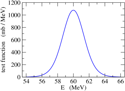
Figure 1: (Color online) The test function defined by Eq. (12). It is obtained with $B$ = 60 MeV, $R$ = 11 fm, $\hbar\Omega$ = 4.5 MeV, and $\Delta E$ = 1.8 MeV.

In order to apply the Bayesian spectral deconvolution to the fusion barrier distributions defined as $d^{2}(E\sigma_{\rm fus})/dE^{2}$, I employ a test function given by,

$$\phi_{k}(E;B_{k},R_{k},\Omega_{k}) = \frac{1}{(\Delta E)^{2}}\,[(E\sigma_{\rm fus})_{E+\Delta E}-2(E\sigma_{\rm fus})_{E}$$ (12)

$$+(E\sigma_{\rm fus})_{E-\Delta E}],$$

where the fusion cross sections $\sigma_{\rm fus}(E)$ is given as,

$$\sigma_{\rm fus}(E)=\frac{\hbar\Omega_{k}}{2E}R_{k}^{2}\,\ln\left[1+\exp\left(\frac{2\pi}{\hbar\Omega_{k}}(E-B_{k})\right)\right],$$ (13)

using the Wong formula Wong73 ; RH15 . In Eq. (12), the second derivative is evaluated with a point difference formula with the energy step $\Delta E$, as has been done in the experimental analyses DHRS98 ; Leigh95 . An example of the test function is shown in Fig. 1, which is obtained with $B$ = 60 MeV, $R$ = 11 fm, $\hbar\Omega$ = 4.5 MeV, and $\Delta E$ = 1.8 MeV. One can see that the test function is centered at $E=B$ with the full-width at half maximum of the order of 0.5$\hbar\Omega$ RSS91 . Notice that with Eqs. (1), (12) and (13), the independent parameters in this analysis read $\tilde{\mbox{\boldmath$\theta$}}=\{\tilde{\mbox{\boldmath$w$}},\mbox{\boldmath$B$},\mbox{\boldmath$R$}\}$, where $\tilde{w}_{k}$ is defined as $\tilde{w}_{k}\equiv w_{k}R_{k}^{2}$.

In the analyses given below, I take the prior probability distribution, $P(\tilde{\mbox{\boldmath$\theta$}})$, in Eq. (7) as a uniform distribution in the rang of $54\leq B_{k}\leq 70$ MeV for ¹⁶O+¹⁴⁴Sm and $50\leq B_{k}\leq 65$ MeV for ¹⁶O+¹⁵⁴Sm, together with $0\leq\tilde{w}_{k}\leq 100$ fm² and $2\leq\hbar\Omega_{k}\leq 5$ MeV (that is, $P(\tilde{\mbox{\boldmath$\theta$}})=0$ if $\tilde{\mbox{\boldmath$\theta$}}$ is outside these ranges). Following Ref. NSO12 , I take $\beta_{l}=1.5^{l-L}$ with $L=24$ except for $l=1$, for which $\beta_{1}$ is taken to be zero. I also follow Ref. NSO12 to take 20000 points in the Metropolis algorithm for each $\beta_{l}$, for which the first 10000 points are thrown away as the burn-in period. For the initial values of the parameters $\tilde{\mbox{\boldmath$\theta$}}$, I take random values according to the probability distribution $P(\tilde{\mbox{\boldmath$\theta$}})$. I find that the results are sometimes improved if this procedure is iterated a few times, that is, if the Metropolis random walk is performed again starting from the optimum values of the parameters obtained in the previous Monte Carlo integration.

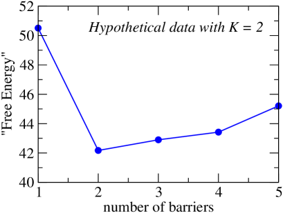
Figure 2: (Color online) The “free energy”, $F(K)=-\ln Z(K)$, as a function of the number of effective barrier, $K$, for hypothetical data generated with $K=2$.

Before I apply this procedure to the actual experimental data, I first carry out a proof-of-principle study by appling the method to hypothetical data generated with Eqs. (1) and (12) with $K=2$, $(\tilde{w}_{1},B_{1},\hbar\Omega_{1})$ = (84.7, 60.0, 4.7), and $(\tilde{w}_{2},B_{2},\hbar\Omega_{2})$ = (33.1, 65.0, 4.2), where $B$ and $\hbar\Omega$ are given in units of MeV while $\tilde{w}$ is given in units of fm². To this end, I generate a data set from $E$=55 MeV to 72 MeV with a step of 0.6 MeV, by adding randomly generated 1% uncertainty in fusion cross sections, which is a typical value in high precision data DHRS98 ; Leigh95 . For the point difference formula for fusion barrier distribution, I take $\Delta E$ = 1.8 MeV, which is the value taken in the experimental analysis for the ¹⁶O+¹⁴⁴Sm system DHRS98 ; Leigh95 . As a result of the Bayesian spectral decomposition for this hypothetical data set, I find that $K$=2 indeed provides the minimum value of “free energy”, $F(K)$, even though $K$=3 also gives a comparable fit (see Fig. 2). The optimum values for the parameters are found to be $(\tilde{w}_{1},B_{1},\hbar\Omega_{1})$ = (84.4$\pm$1.91, 60.0$\pm$0.0301, 4.70$\pm$0.0270), and $(\tilde{w}_{2},B_{2},\hbar\Omega_{2})$ = (25.0$\pm$6.52, 64.5$\pm$0.600, 4.09$\pm$0.338). These values are consistent with the exact values, even though the agreement for the higher peak at $B=65$ MeV is less satisfactory due to larger error bars in the data (notice that the error bar in the barrier distribution increases as a function of energy, see also Fig. 3(c) below). Evidently, the Bayesian spectral deconvolution works well for an analysis of fusion barrier distributions.

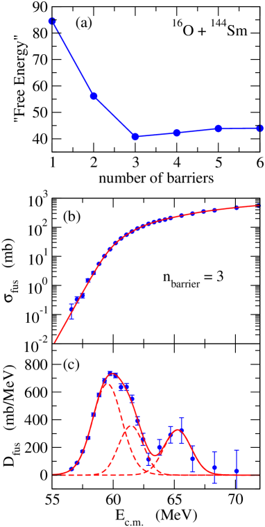
Figure 3: (Color online) Top panel: the “free energy”, $F(K)=-\ln Z(K)$, as a function of the number of effective barrier, $K$, for the ¹⁶O+¹⁴⁴Sm system. Middle panel: the fusion cross sections for the same system. The solid line is obtained with the Bayesian spectral deconvolution with $K$ = 3. Bottom panel: the corresponding barrier distribution defined by $d^{2}(E\sigma_{\rm fus})/dE^{2}$. The contribution of each test function is also shown by the dashed lines. The experimental data are taken from Ref. Leigh95 .

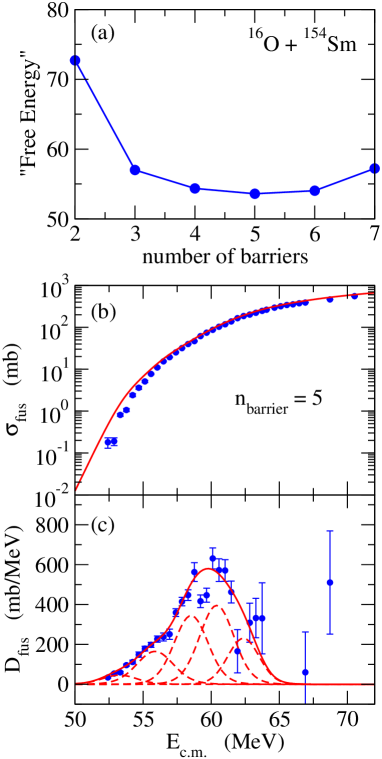
Figure 4: (Color online) Same as Fig. 3, but for the ¹⁶O+¹⁵⁴Sm system. The middle and the bottom panels are obtained with $K=5$.

The posteriori probability of $K$, that is, $P(K|D_{\rm exp})\propto e^{-F(K)}$ (see Eq. (6)), is evaluated as $P(K|D_{\rm exp})$ = 1.32$\times 10^{-4}$, 0.550, 0.266, 0.158, and 0.0264 for $K$ = 1, 2, 3, 4, and 5, respectively. In this paper, $K$=2 has been adopted among those as the optimum value of $K$ according to the idea of maximum-a-posteriori estimate NSO12 . As in Ref. NSO12 , I have repeated the same analysis by generating 100 independent data sets. I have found that the correct value of $K$, that is, $K=2$, is selected 78 times out of 100 while $K$=3 and 4 were selected 19 and 3 times, respectively. The frequency to select the correct value of $K$ (that is, 78%) is significantly larger than the posteriori probability $P(K=2|D_{\rm exp})=55.0\%$, indicating the powerfulness of the present procedure NSO12 .

Let us now analyze the experimental fusion barrier distribution for the ¹⁶O+¹⁴⁴Sm and the ¹⁶O+¹⁵⁴Sm systems. For the latter system, the data points at $E_{\rm c.m.}$ = 59.21 and 59.66 MeV are excluded in the fitting procedure, which appear to deviate from a smooth behavior of barrier distribution. The top panel of Figs. 3 and 4 shows the “free energy” as a function of the number of test function, $K$, thus the number of effective barrier, for the ¹⁶O+¹⁴⁴Sm and the ¹⁶O+¹⁵⁴Sm systems, respectively. It appears that the most probable value of $K$ is $K$ = 3 and 5 for the ¹⁶O+¹⁴⁴Sm and the ¹⁶O+¹⁵⁴Sm systems, respectively. The optimum values of the parameters for these values of $K$ are summarized in Table I (in evaluating the average and the variance for each parameter for the ¹⁶O+¹⁵⁴Sm systems, I have increased the number of Metropolis sampling to 30000 in order to reduce the statistical error). The middle and bottom panels of Figs. 3 and 4 show the fusion cross sections and the fusion barrier distributions obtained with the optimum values of the parameters, respectively. The contribution of each test function is also shown by the dashed lines in the bottom panels. For the ¹⁶O+¹⁴⁴Sm system shown in Fig. 3, one can confirm that the experimental data are well fitted with this procedure. On the other hand, for the ¹⁶O+¹⁵⁴Sm system shown in Fig. 4, the fusion cross sections themselves significantly deviate from the experimental data at low energies, even though the fusion barrier distributrion is well reproduced. This is because the height of the lowest barrier has a large uncertainty (see Table I), to which the fusion cross sections are sensitive at energies well below the Coulomb barrier.

Table 1: The optimum values for the fitting parameters obtained with the Bayesian spectral deconvolution. $K$ is the number of barrier and $w_{k}$ is the weight factor for each barrier. $B_{k}$, $R_{k}$, and $\hbar\Omega_{k}$ are the height, the position, and the curvature of each barrier, respectively.

System	$K$	$B_{k}$ (MeV)	$w_{k}R_{k}^{2}$ (fm2)	$\hbar\Omega_{k}$ (MeV)
16O+144Sm	3	59.5$\pm$0.0789	64.3$\pm$6.06	3.58$\pm$0.149
		61.5$\pm$0.153	28.6$\pm$6.53	2.34$\pm$0.506
		65.3$\pm$0.251	29.0$\pm$4.63	3.00$\pm$0.338
16O+154Sm	5	53.3$\pm$1.10	4.76$\pm$2.87	3.96$\pm$0.589
		55.9$\pm$0.467	18.3$\pm$3.16	4.40$\pm$0.438
		58.5$\pm$0.758	34.7$\pm$19.4	3.77$\pm$0.786
		60.4$\pm$0.833	40.7$\pm$21.4	3.90$\pm$0.939
		62.4$\pm$0.751	21.4$\pm$10.7	3.25$\pm$0.866

It is interesting to notice that, for the ¹⁶O+¹⁴⁴Sm system shown in Fig. 3, the experimental fusion barrier distribution is consistent with the existence of three effective barriers, even though the experimental data show a clear double-peaked structure. I have confirmed that this conclusion remains the same even if the data point at $E$ = 60.64 MeV is excluded from the fitting. For this system, the two main peaks in the barrier distribution has been interpreted to arise from the strong octupole vibrational excitation in the ¹⁴⁴Sm nucleus Leigh95 . The existence of the third peak in the barrier distribution is consistent with the double-octupole phonon excitations in the ¹⁴⁴Sm nucleus, for which the effect of anharmonicity plays an important role HTK97 . On the other hand, for the the ¹⁶O+¹⁵⁴Sm system shown in Fig. 4, the barrier distribution obtained with the Baysian analysis is consistent with the distribution for a prolately deformed nucleus HT12 . If all the effective barriers arise from the rotational excitations of the ¹⁵⁴Sm nucleus, $K$ = 5 indicates that excitations up to the 8⁺ state plays an important role in the subbarrier fusion of the ¹⁶O+¹⁵⁴Sm system.

In summary, I have applied the Bayesian spectral deconvolution in order to analyze the fusion barrier distributions for the ¹⁶O+^144,154Sm systems. Unlike a naive chi-square minimization, this approach provides a consistent way to determine the number of effective barriers originated from the channel coupling effects. I have successfully extracted the number of barriers from the experimental data. In particular, I have found that the barrier distribution for the ¹⁶O+¹⁴⁴Sm system is consistent with three barriers, which indicates the existence of double octupole vibration in the ¹⁴⁴Sm nucleus. For the ¹⁶O+¹⁵⁴Sm system, on the other hand, I have confirmed the rotational nature of the target excitations. In this way, I have demonstrated the effectiveness of the Bayesian spectral deconvolution for fusion barrier distributions.

In principle, one can perform similar studies also for barrier distributions defined with heavy-ion quasi-elastic scattering at backward angles Timmers95 ; HR04 . It would be an interesting future study to apply the Bayesian spectral deconvolution both to the fusion and to the quasi-elastic barrier distributions for the same systems and discuss the consistency of the barrier parameters in the different reaction processes.

I thank T. Ichikawa for useful discussions and for his careful reading of the manuscript.

References

- (1) E.G. Adelberger et al., Rev. Mod. Phys. 70, 1265 (1998); ibid. 83, 195 (2011).
- (2) A.O. Caldeira and A.J. Leggett, Phys. Rev. Lett. 46, 211 (1981).
- (3) S. Takada and H. Nakamura, J. of Chem. Phys. 100, 98 (1994).
- (4) A. Staszczak, A. Baran, J. Dobaczewski, and W. Nazarewicz, Phys. Rev. C80, 014309 (2009).
- (5) A.B. Balantekin and N. Takigawa, Rev. Mod. Phys. 70, 77 (1998).
- (6) K. Hagino and N. Takigawa, Prog. Theor. Phys. 128, 1001 (2012).
- (7) M. Dasgupta, D.J. Hinde, N. Rowley, and A.M. Stefanini, Annu. Rev. Nucl. Part. Sci. 48, 401 (1998).
- (8) B.B. Back, H. Esbensen, C.L. Jiang, and K.E. Rehm, Rev. Mod. Phys. 86, 317 (2014).
- (9) K. Hagino, N. Rowley, and A.T. Kruppa, Comp. Phys. Comm. 123, 143 (1999).
- (10) C.H. Dasso, S. Landowne, and A. Winther, Nucl. Phys. A405, 381 (1983); ibid. A407, 221 (1983).
- (11) K. Hagino and A.B. Balantekin, Phys. Rev. A70, 032106 (2004).
- (12) N. Rowley, G.R. Satchler, and P.H. Stelson, Phys. Lett. B254, 25 (1991).
- (13) J.R. Leigh et al., Phys. Rev. C52, 3151 (1995).
- (14) K. Nagata, S. Sugita, and M. Okada, Neural Networks 28, 82 (2012).
- (15) E.A. Coello Pérez and T. Papenbrock, Phys. Rev. C92, 064309 (2015).
- (16) R.J. Furnstahl, N. Klco, D.R. Phillips, and S. Wesolowski, Phys. Rev. C92, 024005 (2015).
- (17) S. Wesolowski, N. Klco, R.J. Furnstahl, D.R. Phillips, and A. Thapaliya, J. of Phys. G, in press. arXiv:1511.03618 [nucl-th].
- (18) R. Utama, J. Piekarewicz, and H.B. Prosper, Phys. Rev. C93, 014311 (2016).
- (19) E. Sangaline and S. Pratt, Phys. Rev. C93, 024908 (2016).
- (20) K. Hukushima and K. Nemoto, J. Phys. Soc. Japan 65, 980 (1996).
- (21) C.Y. Wong, Phys. Rev. Lett. 31, 766 (1973).
- (22) N. Rowley and K. Hagino, Phys. Rev. C91, 044617 (2015).
- (23) K. Hagino, N. Takigawa, and S. Kuyucak, Phys. Rev. Lett. 79, 2943 (1997).
- (24) H. Timmers et al., Nucl. Phys. A584, 190 (1995).
- (25) K. Hagino and N. Rowley, Phys. Rev. C69, 054610 (2004).