Top-N Recommendation with Novel Rank Approximation

Abstract

The importance of accurate recommender systems has been widely recognized by academia and industry. However, the recommendation quality is still rather low. Recently, a linear sparse and low-rank representation of the user-item matrix has been applied to produce Top-$N$ recommendations. This approach uses the nuclear norm as a convex relaxation for the rank function and has achieved better recommendation accuracy than the state-of-the-art methods. In the past several years, solving rank minimization problems by leveraging nonconvex relaxations has received increasing attention. Some empirical results demonstrate that it can provide a better approximation to original problems than convex relaxation. In this paper, we propose a novel rank approximation to enhance the performance of Top-$N$ recommendation systems, where the approximation error is controllable. Experimental results on real data show that the proposed rank approximation improves the Top-$N$ recommendation accuracy substantially.

1 Introduction

Learning about users’ preference and making recommendations for them is of great importance in e-commerce, targeted advertising and web search. Recommendation is rapidly becoming one of the most successful applications of data mining and machine learning. The goal of a Top-$N$ recommendation algorithm is to produce a length-$N$ list of recommended items such as movies, music, and so on. Over the years, a number of algorithms have been developed to tackle the Top-$N$ recommendation problem [1]. They make predictions based on the user feedback, for example, purchase, rating, review, click, check-in, etc. The existing methods can be broadly classified into two classes: content-based filtering [2] and collaborating filtering (CF) [3] [4] [5].

Content-based filtering: in this approach, features or descriptions are utilized to describe the items and a user profile or model is built using the past item rating to summarize the types of items this user likes [6]. This approach is based on an underlying assumption that liking a feature in the past leads to liking the feature in the future. Some disadvantages of this approach are: If the content does not contain enough information to discriminate the items, then the recommendation will not be accurate; When there is not enough information to build a solid model for a new user, the recommendation will also be jeopardized.

Collaborating filtering: in this approach, user/item co-rating information is utilized to build models. Specifically, CF relies on the following assumption: if a user A likes some items that are also liked by another user B, A is likely to share the same preference with B on another item [7]. One challenge for CF algorithms is to have the ability to deal with highly sparse data, since users typically rate only a small portion of the available items.

In general, CF methods can be further divided into two categories: nearest-neighborhood-based methods and model-based methods. The first class of methods compute the similarities between the users/items using the co-rating information and new items are recommended based on these similarities [8]. One representative method of this kind is Item-based k-nearest-neighbor (ItemKNN) [9]. On the other hand, model-based methods employ a machine learning algorithm to build a model, which is then used to perform the recommendation task [10]. This model learns the similarities between items or latent factors that explain ratings. For example, matrix factorization (MF) method uncovers a low-rank latent structure of data, approximating the user-item matrix as a product of two factor matrices.

Matrix factorization is popular for collaborative prediction and many works are based on it. For instance, pure singular-value-decomposition-based (PureSVD) [11] MF method represents users and items by the most principal singular vectors of the user-item matrix; weighted regularized matrix factorization (WRMF) [12] method deploys a weighting matrix to discriminate between the contributions from observed purchase/rating activities and unobserved ones.

Recently, a novel Top-$N$ recommendation method has been developed, called LorSLIM [13], which has been shown to achieve good performance on a wide variety of datasets and outperform other state-of-the-art approaches. LorSLIM improves upon the traditional item-based nearest neighbor CF approaches by learning directly from the data, a sparse and low-rank matrix of aggregation coefficients that are analogous to the traditional item-item similarities. It demonstrates that low-rank requirement on the similarity matrix is crucial to improve recommendation quality. Since the rank function can hardly be used directly, the nuclear norm [14] is adopted as a convex relaxation of the matrix rank function in LorSLIM. Although the nuclear norm indeed recovers low-rank matrices in some scenarios [15], some recent work has pointed out that this relaxation may lead to poor solutions [16] [17] [18] [19]. In this paper, we propose a novel relaxation which provides a better approximation to the rank function than the nuclear norm. By using this new approximation in LorSLIM model, we observe significant improvement over the current methods. The main contributions of our paper are as follows:

1. We introduce a novel matrix rank approximation function, whose value can be very close to the real rank. This can be applied in a range of rank minimization problems in machine learning and computer vision.

2. An efficient optimization strategy is designed for this associated nonconvex optimization problem, which admits a closed-form solution to every subproblem.

3. As an illustration, we perform experiments on six real datasets. It indicates that our Top-$N$ recommendation approach considerably outperforms the state-of-the-art algorithms which give similar performances on most datesets. Thus this fundamental enhancement is due to our better rank approximation.

The remainder of this paper is organized as follows. In Section 2, we give some notations. Section 3 describes related work. Section 4 introduces the proposed model. In Section 5, we describe our experimental framework. Experimental results and analysis are presented in Section 6; Section 7 draws conclusions.

2 Notations and Definitions

Let $U=\{u_{1},u_{2},...,u_{m}\}$ and $T=\{t_{1},t_{2},...,t_{n}\}$ represent the sets of all users and all items, respectively. The entire set of user-item purchases/ratings is to be represented by user-item matrix $X$ of size $m\times n$. The value of $x_{ij}$ is 1 or a positive value if user $u_{i}$ has ever purchased/rated item $t_{j}$; otherwise it is $0$. $\mathbf{x}_{i}^{T}$ , the $i$-th row of $X$, denotes the purchase/rating history of user $u_{i}$ on all items. The $j$-th column of $X$ denoted as $\mathbf{x}_{j}$ is the purchase/rating history of all users on item $t_{j}$. The aggregation coefficient matrix is represented as $W$ of size $n\times n$. $\mathbf{w}_{j}$ is a size-$n$ column vector of aggregation coefficients. $\|W\|_{1}=\sum\limits_{i}\sum\limits_{j}|w_{ij}|$ is the $l_{1}$-norm of $W$. $\|W\|_{F}^{2}=\sum\limits_{i}\sum\limits_{j}w_{ij}^{2}$ denotes the squared Frobenius norm of $W$. The nuclear norm of $W$ is $\|W\|_{*}=\sum\limits_{i=1}^{n}\sigma_{i}(W)$, where $\sigma_{i}$ is the $i$-th singular value of $W$. The unit step function $s(x)$ has value 1 for $x>0$ and 0 if $x=0$. The rank of matrix $W$ is $\sum\limits_{i=1}^{n}s(\sigma_{i}(W))$. We use $\sigma(W)$ to denote the vector of all singular values of $W$ in non-increasing order. Moreover, $I$ denotes the identity matrix.

In this paper, we denote all vectors (e.g., $\mathbf{x}_{i}$, $\mathbf{x}_{j}$) with bold lower case letters. We represent all matrices (e.g. $W$, $X$) with upper case letters. A predicted value is represented by having a $\wedge$ mark.

3 Relevant Research

Recently, an interesting Top-$N$ recommendation method, sparse linear methods (SLIM) has been proposed [8] which generates recommendation lists by learning a sparse similarity matrix. SLIM solves the following regularized optimization problem:

(3.1) $$\begin{split}&\min_{W}\frac{1}{2}\|X-XW\|_{F}^{2}+\frac{\beta}{2}\|W\|_{F}^{2}+\lambda\|W\|_{1}\\ &s.t.\quad W\geq 0,\quad diag(W)=0,\end{split}$$

where the first term measures the reconstruction error, $\|W\|_{1}$ enforces the sparsity on $W$, and the second and third terms combine the sparsity-inducing property of $\|W\|_{1}$ with the smoothness of $\|W\|_{F}^{2}$, in a way similar to the elastic net [20]. The first constraint is intended to ensure that the learned coefficients represent positive similarities between items, while the second constraint is applied to avoid the trivial solution in which $W$ is an identity matrix, i.e., an item always recommends itself. It has been shown that SLIM outperforms other Top-$N$ recommendation methods. A drawback of SLIM is that it can only model relations between items that have been co-purchased/co-rated by at least one user [13]. Therefore, it fails to capture the potential dependencies between items that have not been co-rated by at least one user, while modeling relations between items that are not co-rated is essential for good performance of item-based approaches in sparse datasets.

To address the above issue, LorSLIM [13] further considers the low-rank structure of $W$. This idea is inspired by the factor model, which assumes that a few latent variables are responsible for items’ features $F$ and the coefficient matrix factors, $W\approx FF^{T}$, with $F$ being of low-rank. Finally, together with sparsity, it constructs a block diagonal $W$, i.e., the items have been classified into many smaller ”clusters” or categories. This situation happens frequently in real life such as movies, music, books and so on. Therefore, this model promotes the recommendation precision further.

In LorSLIM, the nuclear norm $\|W\|_{*}$ is utilized as a surrogate for the rank of $W$. By comparing $\sum\limits_{i=1}^{n}\sigma_{i}$ with $\sum\limits_{i=1}^{n}s(\sigma_{i})$, we can see that when the singular values are much larger than 1, the nuclear norm approximation deviates from the true rank markedly. The nuclear norm is essentially an $l_{1}$-norm of the singular values and it is well known that $l_{1}$-norm has a shrinkage effect and leads to a biased estimator [21] [22]. Recently, some variations of the nuclear norm have been studied, e.g., some of the largest singular values are subtracted from the nuclear norm in truncated nuclear norm regularization [23]; a soft thresholding rule is applied to all singular values in singular value thresholding algorithm [24]; some generalized nonconvex rank approximations have been investigated in [25] [26]. In some applications, they show good performance; however, these models are either overly simple or only restricted to some specific applications.

In this paper, we develop a more general approach, which directly approximates the rank function with our formulation and optimization. Then we show that better rank approximation can improve the recommendation accuracy substantially.

4 Proposed Framework

4.1 Problem Setup

In this paper, we propose the following continuous function to replace the unit step function $s(x)$ in the definition of the rank function:

(4.2) $$f(x)=\sum_{i}(1-\mathrm{e}^{-|x_{i}|/\delta}),$$

where $\delta>0$ controls the approximation accuracy. Equation (4.2) is similar to the formulation proposed in [27]. For any $\sigma_{i}\in[0,\infty)$, $1-\mathrm{e}^{-\sigma_{i}/\delta}\in[0,1)$, and $\int_{0}^{\infty}|(1-\mathrm{e}^{-\sigma_{i}/\delta})-s(\sigma_{i})|^{2}\,d\sigma_{i}=\frac{\delta}{2}$; hence, for any matrix $X$, $f(\sigma(X))$ approaches its true rank as $\delta$ approaches zero.

There are several motivations behind this formulation. First, it attenuates the contributions from large singular values significantly, thus overcomes the imbalanced penalization of different singular values. Second, by defining $\frac{\partial f(0)}{\partial x_{i}}=\lim\limits_{x_{i}\to 0^{+}}\frac{1}{\delta}\mathrm{e}^{-x_{i}/\delta}=\frac{1}{\delta}$, $f$ is differentiable and concave in $[0,\infty)$. Third, $F(X)=f(\sigma(X))$ is unitarily invariant. The last two properties facilitate subsequent optimization and computation much. Compared to many other approaches [28] [29] [25], this formulation enjoys simplicity and efficacy.

To alleviate the issues associated with the nuclear norm, we solve the following problem for Top-$N$ recommendation task:

(4.3) $$\begin{split}&\min_{W}\frac{1}{2}\|X-XW\|_{F}^{2}+\alpha\|W\|_{1}+\beta\sum\limits_{i=1}^{n}(1-e^{-\sigma_{i}(W)/\delta})\\ &+l_{\mathcal{R}_{+}}(W)\\ &s.t.\quad diag(W)=0.\end{split}$$

Different from [8] [13], we incorporate the nonnegative constraint into the objective function by making use of $l_{\mathcal{R}_{+}}$, which is defined element-wisely as

$$l_{\mathcal{R}_{+}}(x)=\left\{\begin{array}[]{ll}0,&\mbox{if $x\geq 0$};\\ +\infty,&\mbox{otherwise.}\end{array}\right.$$

4.2 Optimization

Since (4.3) is a nonconvex problem, it is hard to solve directly. We introduce auxiliary variables to make the objective function separable and solve the following equivalent problem:

(4.5) $$\begin{split}&\min_{W}\frac{1}{2}\|X-XW\|_{F}^{2}+\alpha\|Z_{1}\|_{1}+\beta\sum\limits_{i=1}^{n}(1-e^{-\sigma_{i}(Z_{2})/\delta})\\ &+l_{\mathcal{R}_{+}}(Z_{3})\\ &s.t.\quad diag(W)=0,\hskip 1.42271ptW=Z_{1},\hskip 1.42271ptW=Z_{2},\hskip 1.42271ptW=Z_{3}.\end{split}$$

This can be solved by using the augmented Lagrange multiplier (ALM) method [30]. We turn to minimizing the following augmented Lagrangian function:

(4.6) $$\mathcal{L}(W,Z_{1},Z_{2},Z_{3})$$

$$=\frac{1}{2}\|X-XW\|_{F}^{2}+\alpha\|Z_{1}\|_{1}+\beta\sum\limits_{i=1}^{n}(1-e^{-\sigma_{i}(Z_{2})/\delta})$$

$$+l_{\mathcal{R}_{+}}(Z_{3})+\frac{\mu}{2}\Big{[}\|Z_{1}-(W-\frac{Y_{1}}{\mu})\|_{F}^{2}+$$

$$\|Z_{2}-(W-\frac{Y_{2}}{\mu})\|_{F}^{2}+\|Z_{3}-(W-\frac{Y_{3}}{\mu})\|_{F}^{2}\Big{]},$$

where $\mu>0$ is the penalty parameter and $Y_{1}$, $Y_{2}$, $Y_{3}$ are the Lagrange multipliers. This unconstrained problem can be minimized with respect to $Z_{1}$, $Z_{2}$, and $Z_{3}$ alternatively, by fixing the other variables, and then updating the Lagrange multipliers $Y_{1}$, $Y_{2}$, and $Y_{3}$. At the $(t+1)$th iteration,

(4.7) $$\begin{split}&W^{t+1}=\operatorname*{arg\,min}_{W}\frac{1}{2}\|X-XW\|_{F}^{2}+\frac{\mu^{t}}{2}\Big{[}\|Z_{1}^{t}-(W-\frac{Y_{1}^{t}}{\mu})\|_{F}^{2}\\ &+\|Z_{2}^{t}-(W-\frac{Y_{2}^{t}}{\mu})\|_{F}^{2}+\|Z_{3}^{t}-(W-\frac{Y_{3}^{t}}{\mu})\|_{F}^{2}\Big{]}\end{split}$$

We can see that the objective function of (4.7) is quadratic and strongly convex in $W$, which has a closed-form solution:

(4.8) $$\begin{split}&W^{t+1}=(3\mu^{t}I+X^{T}X)^{-1}[\mu^{t}(Z_{1}^{t}+Z_{2}^{t}+Z_{3}^{t})+\\ &(Y_{1}^{t}+Y_{2}^{t}+Y_{3}^{t})+X^{T}X].\end{split}$$

For $Z_{1}$ minimization, we have

(4.9) $$Z_{1}^{t+1}=\operatorname*{arg\,min}_{Z_{1}}\alpha\|Z_{1}\|_{1}+\frac{\mu^{t}}{2}\left\|Z_{1}-(W^{t+1}-\frac{Y_{1}^{t}}{\mu})\right\|_{F}^{2},$$

which can be solved by the following lemma [31].

Lemma 4.1

For $\mu>0$ and $Y\in\mathcal{R}^{m\times n}$, the solution of the problem

$$\min_{X}\mu\|X\|_{1}+\frac{1}{2}\|X-Y\|_{F}^{2}$$

is given by $X_{\mu}(Y)$, which is defined component-wisely by

$$[X_{\mu}(Y)]_{ij}=\textrm{max}\{|y_{ij}|-\mu,0\}\cdot sign(y_{ij}).$$

Therefore, by letting $Q=W^{t+1}-\frac{Y_{1}^{t}}{\mu^{t}}$, we can solve $Z_{1}$ element-wisely as below:

(4.10) $$(Z_{1}^{t+1})_{ij}=\textrm{max}(|Q_{ij}|-\alpha/\mu^{t},0)\cdot sign(Q_{ij}).$$

To update $Z_{2}$, we have

(4.11) $$\min_{Z_{2}}\beta\sum\limits_{i=1}^{n}(1-e^{-\sigma_{i}(Z_{2})/\delta})+\frac{\mu^{t}}{2}\|Z_{2}-(W^{t+1}-\frac{Y_{2}^{t}}{\mu^{t}})\|_{F}^{2},$$

This can be solved with the following theorem.

Theorem 4.1

[32] If $F(Z)=f(\sigma(Z))$ is a unitarily invariant function, $\mu>0$, and $A\in\mathbf{\mathcal{R}}^{m\times n}$ whose SVD is $U\Sigma_{A}V^{T}$ and $\Sigma_{A}=diag(\sigma_{A})$ , then the optimal solution to the following problem

(4.12) $$\min_{Z}F(Z)+\frac{\mu}{2}\left\|Z-A\right\|_{F}^{2},$$

is $Z^{*}$ with SVD being $U\Sigma_{Z}^{*}V^{T}$, where $\Sigma_{Z}^{*}=diag(\sigma^{*})$ is obtained through the Moreau-Yosida operator $\sigma^{*}=\mathrm{prox}_{f,\mu}(\sigma_{A})$, defined as

(4.13) $$\mathrm{prox}_{f,\mu}(\sigma_{A}):=\operatorname*{arg\,min}_{\sigma\geq 0}f(\sigma)+\frac{\mu}{2}\|\sigma-\sigma_{A}\|_{2}^{2}.$$

In our case, the first term in (4.13) is concave while the second term is convex in $\sigma$, so we can resort to the difference of convex (DC) [33] optimization strategy. A linear approximation is applied at each iteration of DC programing. For this inner loop, at the $(k+1)$th iteration,

(4.14) $$\sigma^{k+1}=(\sigma_{A}-\frac{\beta\omega_{k}}{\mu^{t}})_{+},$$

where $\omega_{k}=\partial f(\sigma^{k})$ is the gradient of $f(\cdot)$ at $\sigma^{k}$ and $Udiag\{\sigma_{A}\}V^{T}$ is the SVD of $W^{t+1}-\frac{Y_{2}^{t}}{\mu^{t}}$. Finally, it converges to a local optimal point $\sigma^{*}$. Then $Z_{2}^{t+1}=Udiag\{\sigma^{*}\}V^{T}$.

To update $Z_{3}$, we need to solve

(4.15) $$Z_{3}^{t+1}=\operatorname*{arg\,min}_{Z_{3}}l_{\mathcal{R}_{+}}(Z_{3})+\frac{\mu^{t}}{2}\|Z_{3}-(W^{t+1}-\frac{Y_{3}^{t}}{\mu^{t}})\|_{F}^{2},$$

which yields the updating rule

(4.16) $$Z_{3}^{t+1}=\textrm{max}(W^{t+1}-\frac{Y_{3}^{t}}{\mu^{t}},0).$$

Here max$(\cdot)$ is an element-wise operator. The complete procedure is outlined in Algorithm 1.

Algorithm 1 Solve (4.3)

Input: Original data matrix $X\in\mathbf{\mathcal{R}}^{m\times n}$, parameters $\alpha>0$, $\beta>0$, $\mu^{0}>0$, $\gamma>1$.
Initialize: $Z_{1}=Z_{2}=Z_{3}$ as $n$-by-$n$ matrices with random numbers between 0 and 1, $Y_{1}=Y_{2}=Y_{3}=0$.
REPEAT

1:  Obtain $W$ through (4.8).

2:  Update $Z_{1}$ as (4.10).

3:  Solve $Z_{2}$ by solving (4.11).

4:  Update $Z_{3}$ as (4.16).

5:  Update the Lagrangian multipliers:

$$Y_{1}^{t+1} =Y_{1}^{t}+\mu^{t}(Z_{1}^{t+1}-W^{t+1}),$$

$$Y_{2}^{t+1} =Y_{2}^{t}+\mu^{t}(Z_{2}^{t+1}-W^{t+1}),$$

$$Y_{3}^{t+1} =Y_{3}^{t}+\mu^{t}(Z_{3}^{t+1}-W^{t+1}).$$

6:  Update the parameter $\mu^{t}$ by $\mu^{t+1}=\gamma\mu^{t}$.

UNTIL stopping criterion is met.

5 Experimental Evaluation

5.1 Datasets

Table 1: The datasets used in evaluation

dataset	#users	#items	#trns	rsize	csize	density	ratings
Delicious	1300	4516	17550	13.50	3.89	0.29%	-
lastfm	8813	6038	332486	37.7	55.07	0.62%	-
BX	4186	7733	182057	43.49	23.54	0.56%	-
ML100K	943	1682	100000	106.04	59.45	6.30%	1-10
Netflix	6769	7026	116537	17.21	16.59	0.24%	1-5
Yahoo	7635	5252	212772	27.87	40.51	0.53%	1-5

• The “#users”, “#items”, “#trns” columns show the number of users, number of items and number of transactions, respectively, in each dataset. The “rsize” and “csize” columns show the average number of ratings of each user and of each item, respectively, in each dataset. Column corresponding to “density” shows the density of each dataset (i.e., density=#trns/(#users$\times$#items)). The “ratings” column is the rating range of each dataset with granularity 1.

We evaluate the performance of our method on six different real datasets whose characteristics are summarized in Table 1. These datasets represent different applications of a recommendation algorithm. They can be broadly categorized into two classes.

The first class contains Delicious, lastfm and BX. These three datasets have only implicit feedback, i.e., they are represented by binary matrices. Specifically, Delicious was the bookmarking and tagging information of 2$K$ users in Delicious social bookmarking system, in which each URL was bookmarked by at least 3 users. Lastfm represents music artist listening information extracted from the last.fm online music system, in which each music artist was listened to by at least 10 users and each user listened to at least 5 artists. BX is a part of the Book-Crossing dataset such that only implicit interactions were contained and each book was read by at least 10 users.

The second class contains ML100K, Netflix and Yahoo. All these datasets contain multi-value ratings. Specifically, the ML100K dataset contains movie ratings and is a subset of the MovieLens research project. The Netflix is a subset of Netflix Prize dataset and each user rated at least 10 movies. The Yahoo dataset is a subset obtained from Yahoo!Movies user ratings. In this dataset, each user rated at least 5 movies and each movie was rated by at least 3 users.

Table 2: Comparison of Top-N recommendation algorithms

method	Delicious							lastfm
	params				HR	ARHR		params				HR	ARHR
ItemKNN	300	-	-	-	0.300	0.179		100	-	-	-	0.125	0.075
PureSVD	1000	10	-	-	0.285	0.172		200	10	-	-	0.134	0.078
WRMF	250	5	-	-	0.330	0.198		100	3	-	-	0.138	0.078
BPRKNN	1e-4	0.01	-	-	0.326	0.187		1e-4	0.01	-	-	0.145	0.083
BPRMF	300	0.1	-	-	0.335	0.183		100	0.1	-	-	0.129	0.073
SLIM	10	1	-	-	0.343	0.213		5	0.5	-	-	0.141	0.082
LorSLIM	10	1	3	3	0.360	0.227		5	1	3	3	0.187	0.105
Our	20	5	20	-	0.385	0.232		10	0.1	10	-	0.210	0.123
method	BX							ML100K
	params				HR	ARHR		params				HR	ARHR
ItemKNN	400	-	-	-	0.045	0.026		10	-	-	-	0.287	0.124
PureSVD	3000	10	-	-	0.043	0.023		100	10	-	-	0.324	0.132
WRMF	400	5	-	-	0.047	0.027		50	1	-	-	0.327	0.133
BPRKNN	1e-3	0.01	-	-	0.047	0.028		2e-4	1e-4	-	-	0.359	0.150
BPRMF	400	0.1	-	-	0.048	0.027		200	0.1	-	-	0.330	0.135
SLIM	20	0.5	-	-	0.050	0.029		2	2	-	-	0.343	0.147
LorSLIM	50	0.5	2	3	0.052	0.031		10	8	5	3	0.397	0.207
Our	1	1	10	-	0.061	0.038		200	0.2	700	-	0.434	0.224
method	Netflix							Yahoo
	params				HR	ARHR		params				HR	ARHR
ItemKNN	200	-	-	-	0.156	0.085		300	-	-	-	0.318	0.185
PureSVD	500	10	-	-	0.158	0.089		2000	10	-	-	0.210	0.118
WRMF	300	5	-	-	0.172	0.095		100	4	-	-	0.250	0.128
BPRKNN	2e-3	0.01	-	-	0.165	0.090		0.02	1e-3	-	-	0.310	0.182
BPRMF	300	0.1	-	-	0.140	0.072		300	0.1	-	-	0.308	0.180
SLIM	5	1.0	-	-	0.173	0.098		10	1	-	-	0.320	0.187
LorSLIM	10	3	5	3	0.196	0.111		10	1	2	3	0.334	0.191
Our	200	100	200	-	0.228	0.122		300	10	100	-	0.360	0.205

• The parameters for each method are described as follows: ItemKNN: the number of neighbors $k$; PureSVD: the number of singular values and the number of SVD; WRMF: the dimension of the latent space and its weight on purchases; BPRKNN: its learning rate and regularization parameter $\lambda$; BPRMF: the latent space’s dimension and learning rate; SLIM: the $l_{2}$-norm regularization parameter $\beta$ and the $l_{1}$-norm regularization coefficient $\lambda$; LorSLIM: the $l_{2}$-norm regularization parameter $\beta$, the $l_{1}$-norm regularization parameter $\lambda$, the nuclear norm regularization coefficient $z$ and the auxiliary parameter $\rho$. Our: the $l_{1}$-norm regularization parameter $\alpha$, the rank regularization parameter $\beta$ and the auxiliary parameter $\mu^{0}$. $N$ in this table is 10. Bold numbers are the best performance in terms of HR and ARHR for each dataset.

5.2 Evaluation Methodology

To examine the effectiveness of the proposed method, we follow the procedure in [8] and adopt 5-fold cross validation. For each fold, a dataset is split into training and test sets by randomly selecting one non-zero entry for each user and putting it in the test set, while using the rest of the data for training the model. Then a ranked list of size-$N$ items for each user is produced. We then evaluate the model by comparing the ranked list of recommended items with the item in the test set. In the following results presented in this paper, $N$ is equal to 10 by default.

The recommendation quality is evaluated by the Hit Rate (HR) and the Average Reciprocal Hit Rank (ARHR) [9]. HR is defined as

(5.17) $$HR=\frac{\#\textrm{hits}}{\#\textrm{users}},$$

where #hits is the number of users whose item in the testing set is contained (i.e., hit) in the size-$N$ recommendation list, and #users is the total number of users. An HR value of 1.0 means that the algorithm is able to always recommend hidden items correctly, whereas an HR value of 0.0 indicates that the algorithm is not able to recommend any of the hidden items.

A drawback of HR is that it treats all hits equally without considering where they appear in the Top-$N$ list. ARHR addresses this by rewarding each hit based on its place in the Top-$N$ list, which is defined as:

(5.18) $$ARHR=\frac{1}{\#\textrm{users}}\sum_{i=1}^{\#\textrm{hits}}\frac{1}{p_{i}},$$

where $p_{i}$ is the position of the item in the ranked Top-$N$ list for the $i$-th hit. In this metric, hits that occur earlier in the ranked list are weighted higher than those occur later, and thus ARHR indicates how strongly an item is recommended. The highest value of ARHR is equal to HR which occurs when all the hits occur in the first position, and the lowest value is equal to HR/$N$ when all the hits occur in the last position of the list.

HR and ARHR are recommended as evaluation metrics since they directly measure the performance based on the ground truth data, i.e., what users have already provided feedback [8].

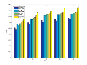
(a) Delicious

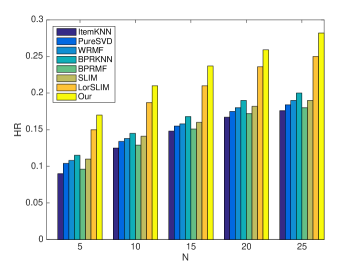
(b) lastfm

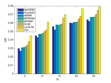
(c) BX

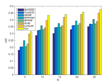
(d) ML100K

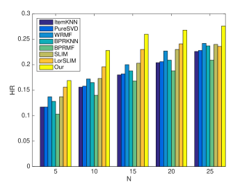
(e) Netflix

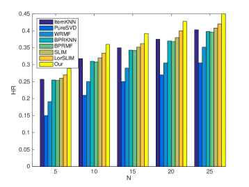
(f) Yahoo

Figure 1: Performance for Different Values of $N$.

5.3 Comparison Algorithms

We compare the performance of the proposed method with seven state-of-the-art Top-$N$ recommendation algorithms, including the item neighborhood-based collaborative filtering method ItemKNN [9], two MF-based methods PureSVD [11] and WRMF [34], SLIM [8] and LorSLIM [13]. We also examine two ranking/retrieval criteria based methods BPRMF and BPRKNN [35], where Bayesian personalized ranking (BPR) criterion is used which measures the difference between the rankings of user-purchased items and the remaining items.

6 Results

6.1 Top-N Recommendation Performance

We summarize the experimental results of different methods in Table 2. It shows that our algorithm performs the best among all methods across all the datasets. Specifically, in terms of HR, our method outperforms ItemKNN, PureSVD, WRMF, BPRKNN, BPRMF, SLIM and LorSLIM by 40.41%, 47.22%, 34.65%, 27.99%, 36.01%, 25.67%, 11.66% on average, respectively, over all the six datasets; with respect to ARHR, the average improvements across all the datasets for ItemKNN, PureSVD, WRMF, BPRKNN, BPRMF, SLIM and LorSLIM are 45.79%, 56.38%, 45.43%, 34.25%, 46.71%, 29.41%, 11.23%, respectively. This suggests that a closer rank approximation than the nuclear norm is indeed crucial in real applications.

Among seven other algorithms, LorSLIM is a little better than the others. SLIM, BPRMF, and BPRKNN give similar performance. For the three MF-based methods, BPRMF and WMF are better than PureSVD except on lastfm and ML100K. It is interesting to note that the simple itemKNN performs better than BPRMF on Netflix and Yahoo. This could be because in BPRMF , the entire AUC curve is used to measure if the interested items are ranked higher than the rest. However, a good AUC value may not lead to good performance for Top-$N$ recommendation [35].

6.2 Recommendation for Different Top-N

We show the performance of these algorithms for different values of $N$ (i.e., 5, 10, 15, 20 and 25) on all six datasets in Figure 1. It shows that our algorithm outperforms other methods significantly in all cases. Once again, it demonstrates the importance of good rank approximation.

6.3 Matrix Reconstruction

We use ML100K to show how LorSLIM and our method reconstruct the user-item matrix. The density of ML100K is 6.30% and the mean for those non-zero elements is 3.53. The reconstructed matrix $\hat{X}_{LorSLIM}$ from LorSLIM has a density of 13.61%, whose non-zero values have a mean of 0.046. For those 6.30% non-zero entries in $X$, $\hat{X}_{LorSLIM}$ recovers 70.68% of them and their mean value is 0.0665. In contrast, our proposed algorithm recovers all zero values. The mean of our reconstructed matrix is 0.236. For those 6.30% non-zero entries in $X$, it gives a mean of 1.338. These facts suggest that our method better recovers $X$ than LorSLIM can do. In other words, LorSLIM loses too much information. This appears to explain the superior performance of our proposed method.

6.4 Parameter Effects

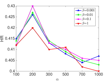
Figure 2: Influence of $\alpha$ and $\beta$ on HR for ML100K dataset.

Our model involves parameters $\alpha$, $\beta$. We also introduce an auxiliary parameter $\mu$ in ALM algorithm. Some previous studies have pointed out that a dynamical $\mu$ is preferred in practice. Hence we increase $\mu$ at a rate of $\gamma$ with a value 1.1, which is a popular choice in the literature. For each possible combination of $\alpha$, $\beta$, we can use grid search to find the optimal initial value $\mu^{0}$.

In Figure 2, we depict the effects of different $\alpha$, $\beta$ on dataset ML100K. As can be seen from it, our algorithm performs well over a large range of $\alpha$ and $\beta$. Compared to $\beta$, the result is more sensitive to $\alpha$. The performance keeps increasing as $\alpha$ increase when it is small, then decreases as it become larger. This is because the $l_{1}$-norm parameter $\alpha$ controls the sparsity of the aggregating matrix. If $\alpha$ is too large, the matrix will be too sparse that nearly no item will be recommended since the coefficients with the target item are all zero.

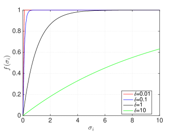
Figure 3: Effect of $\delta$ on rank approximation.

Another important parameter is $\delta$ in our rank approximation, which measures how close of our rank relaxation to the true rank. Generally speaking, it is always safe to choose a small value, although $\delta$ can be big if the singular values are big or the size of matrix is big. If $\delta$ is too small, it may incur some numerical issues. Figure 3 displays the influence of $\delta$ on the rank approximation. It can be seen that $f$ can match the rank function closely when $\delta\leq 0.1$. For our previous experimental results, $\delta=0.1$ is applied, which results in an approximation error of $0.05$.

7 Conclusion

In this paper, we propose a novel rank relaxation to solve the Top-$N$ recommendation problem. This approximation addresses the limitations of the nuclear norm by mimicing the behavior of the true rank function. We show empirically that this nonconvex rank approximation can substantially improve the quality of Top-$N$ recommendation. This surrogate for the rank function of a matrix may as well benefit a number of other problems, such as robust PCA and robust subspace clustering.

8 Acknowledgments

This work is supported by the U.S. National Science Foundation under Grant IIS 1218712.

References

- [1] F. Ricci, L. Rokach, and B. Shapira, Introduction to recommender systems handbook. Springer, 2011.
- [2] M. Balabanović and Y. Shoham, “Fab: content-based, collaborative recommendation,” Communications of the ACM, vol. 40, no. 3, pp. 66–72, 1997.
- [3] Q. Gu, J. Zhou, and C. H. Ding, “Collaborative filtering: Weighted nonnegative matrix factorization incorporating user and item graphs.” in SDM. SIAM, 2010, pp. 199–210.
- [4] F. Wang, S. Ma, L. Yang, and T. Li, “Recommendation on item graphs,” in Data Mining, 2006. ICDM’06. Sixth International Conference on. IEEE, 2006, pp. 1119–1123.
- [5] S. Zhang, W. Wang, J. Ford, and F. Makedon, “Learning from incomplete ratings using non-negative matrix factorization.” in SDM, vol. 6. SIAM, 2006, pp. 548–552.
- [6] M. J. Pazzani and D. Billsus, “Content-based recommendation systems,” in The adaptive web. Springer, 2007, pp. 325–341.
- [7] C. Desrosiers and G. Karypis, “A comprehensive survey of neighborhood-based recommendation methods,” in Recommender systems handbook. Springer, 2011, pp. 107–144.
- [8] X. Ning and G. Karypis, “Slim: Sparse linear methods for top-n recommender systems,” in Data Mining (ICDM), 2011 IEEE 11th International Conference on. IEEE, 2011, pp. 497–506.
- [9] M. Deshpande and G. Karypis, “Item-based top-n recommendation algorithms,” ACM Transactions on Information Systems (TOIS), vol. 22, no. 1, pp. 143–177, 2004.
- [10] Z. Kang, C. Peng, and Q. Cheng, “Top-n recommender system via matrix completion,” in Thirtieth AAAI Conference on Artificial Intelligence, 2016.
- [11] P. Cremonesi, Y. Koren, and R. Turrin, “Performance of recommender algorithms on top-n recommendation tasks,” in Proceedings of the fourth ACM conference on Recommender systems. ACM, 2010, pp. 39–46.
- [12] R. Pan, Y. Zhou, B. Cao, N. N. Liu, R. Lukose, M. Scholz, and Q. Yang, “One-class collaborative filtering,” in Data Mining, 2008. ICDM’08. Eighth IEEE International Conference on. IEEE, 2008, pp. 502–511.
- [13] Y. Cheng, L. Yin, and Y. Yu, “Lorslim: Low rank sparse linear methods for top-n recommendations,” in Data Mining (ICDM), 2014 IEEE International Conference on. IEEE, 2014, pp. 90–99.
- [14] B. Recht, M. Fazel, and P. A. Parrilo, “Guaranteed minimum-rank solutions of linear matrix equations via nuclear norm minimization,” SIAM review, vol. 52, no. 3, pp. 471–501, 2010.
- [15] E. J. Candès and B. Recht, “Exact matrix completion via convex optimization,” Foundations of Computational mathematics, vol. 9, no. 6, pp. 717–772, 2009.
- [16] X. Shi and P. S. Yu, “Limitations of matrix completion via trace norm minimization,” ACM SIGKDD Explorations Newsletter, vol. 12, no. 2, pp. 16–20, 2011.
- [17] Z. Kang, C. Peng, and Q. Cheng, “Robust pca via nonconvex rank approximation,” in Data Mining (ICDM), 2015 IEEE International Conference on, Nov 2015, pp. 211–220.
- [18] Z. Kang and Q. Cheng, “Robust subspace clustering via tighter rank approximation,” in Proceedings of the 24th ACM International on Conference on Information and Knowledge Management. ACM, 2015, pp. 393–401.
- [19] N. Srebro and R. R. Salakhutdinov, “Collaborative filtering in a non-uniform world: Learning with the weighted trace norm,” in Advances in Neural Information Processing Systems, 2010, pp. 2056–2064.
- [20] H. Zou and T. Hastie, “Regularization and variable selection via the elastic net,” Journal of the Royal Statistical Society: Series B (Statistical Methodology), vol. 67, no. 2, pp. 301–320, 2005.
- [21] J. Fan and R. Li, “Variable selection via nonconcave penalized likelihood and its oracle properties,” Journal of the American statistical Association, vol. 96, no. 456, pp. 1348–1360, 2001.
- [22] C.-H. Zhang, “Nearly unbiased variable selection under minimax concave penalty,” The Annals of Statistics, pp. 894–942, 2010.
- [23] Y. Hu, D. Zhang, J. Ye, X. Li, and X. He, “Fast and accurate matrix completion via truncated nuclear norm regularization,” Pattern Analysis and Machine Intelligence, IEEE Transactions on, vol. 35, no. 9, pp. 2117–2130, 2013.
- [24] J.-F. Cai, E. J. Candès, and Z. Shen, “A singular value thresholding algorithm for matrix completion,” SIAM Journal on Optimization, vol. 20, no. 4, pp. 1956–1982, 2010.
- [25] C. Lu, J. Tang, S. Yan, and Z. Lin, “Generalized nonconvex nonsmooth low-rank minimization,” in Computer Vision and Pattern Recognition (CVPR), 2014 IEEE Conference on. IEEE, 2014, pp. 4130–4137.
- [26] C. Lu, C. Zhu, C. Xu, S. Yan, and Z. Lin, “Generalized singular value thresholding,” in Twenty-Ninth AAAI Conference on Artificial Intelligence, 2015.
- [27] M. Malek-Mohammadi, M. Babaie-Zadeh, and M. Skoglund, “Iterative concave rank approximation for recovering low-rank matrices,” Signal Processing, IEEE Transactions on, vol. 62, no. 20, pp. 5213–5226, 2014.
- [28] Z. Kang, C. Peng, and Q. Cheng, “Robust subspace clustering via smoothed rank approximation,” SIGNAL PROCESSING LETTERS, IEEE, vol. 22, no. 11, pp. 2088–2092, Nov 2015.
- [29] C. Peng, Z. Kang, H. Li, and Q. Cheng, “Subspace clustering using log-determinant rank approximation,” in Proceedings of the 21th ACM SIGKDD International Conference on Knowledge Discovery and Data Mining. ACM, 2015, pp. 925–934.
- [30] D. P. Bertsekas, “Nonlinear programming,” 1999.
- [31] A. Beck and M. Teboulle, “A fast iterative shrinkage-thresholding algorithm for linear inverse problems,” SIAM journal on imaging sciences, vol. 2, no. 1, pp. 183–202, 2009.
- [32] Z. Kang, C. Peng, J. Cheng, and Q. Cheng, “Logdet rank minimization with application to subspace clustering,” Computational Intelligence and Neuroscience, vol. 2015, 2015.
- [33] R. Horst and N. V. Thoai, “Dc programming: overview,” Journal of Optimization Theory and Applications, vol. 103, no. 1, pp. 1–43, 1999.
- [34] Y. Hu, Y. Koren, and C. Volinsky, “Collaborative filtering for implicit feedback datasets,” in Data Mining, 2008. ICDM’08. Eighth IEEE International Conference on. IEEE, 2008, pp. 263–272.
- [35] S. Rendle, C. Freudenthaler, Z. Gantner, and L. Schmidt-Thieme, “Bpr: Bayesian personalized ranking from implicit feedback,” in Proceedings of the Twenty-Fifth Conference on Uncertainty in Artificial Intelligence. AUAI Press, 2009, pp. 452–461.