Probing quantum gravity effects with ion trap

Abstract

The existence of minimal length scale has motivated the proposal of generalized uncertainty principle, which provides a potential routine to probe quantum gravitational effects in low-energy quantum mechanics experiment. Hitherto, the tabletop experiment of testing deviations from ordinary quantum mechanics are mostly based on microscopic objects. However, the feasibility of these studies are challenged by the recent study of spacetime quantization for composite macroscopic body. In this paper, we propose a scheme to probe quantum gravity effects by revealing the deviations from predictions of Heisenberg uncertainty principle. Our scheme focus on manipulating the interaction sequences between external laser fields and a single trapped ion to seek evidence of spacetime quantization, therefore reduce the complicity induced by large bodies to some extent. The relevant study for microscopic particles is crucial considering the lack of satisfactory theories regarding basic properties for multi-particles in the framework of quantum gravity. Meanwhile, we are managed to set a new upper limit for deformation parameter.

year number number identifier Date text]date LABEL:FirstPage1 LABEL:LastPage#1102

I Introduction

Quantum gravity is referred to a theory unifying the general relativity and quantum mechanics. The primary obstacle in developing such a theory is lacking testable experiments of quantum gravitational effects. Previously studies are usually based on high-energy astronomical events A ; U ; F with energy in the order of $E_{p}=c\hbar/L_{p}=1.2\times 10^{19}$ GeV, where the general relativity are expected to merge with quantum physics. While the emergence of a minimal length scale predicted by various approaches to quantum gravity provides possibilities to find first ever experimental evidence in low-energy quantum mechanics realm. Specifically, the existence of minimal length scale is against the Heisenberg uncertainty relation and motivates the proposal of a generalized uncertainty principle (GUP). Thus, it’s generally believed that quantum gravity can be tested to perform high-sensitivity measurement of the uncertainty relation. In this sense, many proposals are aimed to disclose derivations from the predictions of ordinary quantum mechanics (QM) based on uncertainty relation. This motivated a growing number of approaches to search for evidence of Planck-scale physics which raised the hope to get experimental direct access to the gravity induced effects.

Refs.J expounded the feasibility of study Planck-scale physics in a tabletop experiment by observing the motion of a dielectric macroscopic block through a distance of the order of Planck’s length. Refs. I proposed schemes to measure possible Planck-scale deformation with optomechanics in an unprecedented sensitivity. Ref. M measured the change in the oscillator ground-state energy induced by modified commutator with gravitational bar detectors. All those proposals are based on the consensus that the quantization of spacetime for macroscopic objects is same as that for its constituent particles. However, Camelia challenged this assertion and point out that the spacetime quantization is much weaker for center-of-mass of a macroscopic body compared with fundamental particles constitute it Camelia . According to the conclusion of Camelia, new approaches pertaining fundamental particles should be came up with to detect quantum gravity effects, instead of focusing on schemes concerning the center-of-mass motions of macroscopic objects.

The ion trap system has been widely studied for its many advantages like long coherent time. In this paper, we propose a scheme to detect the quantum gravity effects with a two-level ion trapped in a Paul trap. By manipulating the phase of classical laser addressing the ion, a sequence of four interactions between ion and laser is designed such that a phase is accumulated on a specific ground state during the oscillating period of ion external motion. By repeating the cycle and controlling cycle times, the phase obtained by standard quantum mechanics is washed out and thus the deformation related phase corresponding to the derivation result from quantum gravity effects can be extracted. After a Hadmard transformation with another auxiliary level, the deformation of phase is mapped into the population change, which can be detected with a high accuracy. In the case of a null result of detection, an upper bound for $\beta_{0}$ can be set. In this way, we provide a method to perfect the quantum gravity theories with empirical feed back. Moreover, since only a single ion is concerned, our scheme can avoid the errors referred in Camelia introduced by macroscopic probes.

II The generalized uncertainty principle

The Heisenberg uncertainty principle allows localizing a particle sharply at a point at the expense of the information on the conjugate momentum. While when quantum gravity is considered, uncertainty principle need to be generalized to incorporate the effect of minimal length scale GUP .

$$\Delta\hat{x}\Delta\hat{p}\geq\frac{\hbar}{2}(1+\beta_{0}(\frac{\Delta\hat{p}}{M_{p}c})^{2}),$$ (1)

where $\beta_{0}$ is the deformed parameters that quantifies the modification strength, $M_{p}$ is the Planck mass and $M_{p}c^{2}$ is Planck energy $E_{p}$. It has been proved that GUP is equivalent to a modified canonical commutator in the following form K ,

$$[\hat{x},\hat{p}]=i\hbar(1+\beta_{0}(\frac{\hat{p}}{M_{p}c})^{2}).$$ (2)

Let us define S

$$\hat{x}=x,\hat{p}=p(1+\frac{1}{3}\beta p^{3}).$$ (3)

The operators with and without a hat represent deformed and standard operators respectively, and $\beta=\frac{\beta_{0}}{M_{p}c}$. Note that, the modified Heisenberg algebra (2) is satisfied to order $\beta$, we thus neglect the terms of higher order throughout the paper.

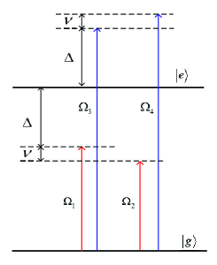
Figure 1: (color online) The energy levels of the trapped ion and the transition driven by four classical lasers. The ion is illuminated by lasers with opposite detuning.

Next, we proceed to elaborate our scheme to measure deformations from ordinary QM. Considering a two-level ion trapped in a Paul trap, the transition between ground state $\left|g\right\rangle$ and exited state $\left|e\right\rangle$ is driven by four laser fields with frequency $\omega_{i}$ $(i=1,2,3,4),$ as shown in Fig.1. $\omega_{1},\omega_{2}$ are respectively detuned by $\Delta_{1}$ and $\Delta_{2}$ from the $\left|g\right\rangle\leftrightarrow\left|e\right\rangle$ transition and have a relative detuning $\Delta\omega=\omega_{1}-\omega_{2}=\nu$, equivalent to the frequency of the vibrational mode of the ion. The frequencies $\omega_{3},\omega_{4}$ have the opposite detuning corresponding to $\omega_{1},\omega_{2}$ respectively while the same relative detuning $\Delta\omega=\omega_{4}-\omega_{3}=\nu.$ The total Hamiltonian of the system in the framework of GUP takes the form

$$H = \hbar\omega_{eg}\left|e\right\rangle\left\langle e\right|+\frac{\hat{p}^{2}}{2m}+\frac{m\omega^{2}\hat{x}^{2}}{2}$$ (5)

$$+\sum_{m=1}^{4}\frac{\hbar\Omega_{m}}{2}e^{i\omega_{m}t+i\overrightarrow{k}_{m}\cdot\overrightarrow{\hat{r}}+i\phi_{m}}\left|e\right\rangle\left\langle g\right|+\text{H}.\text{c}.$$

$$= \hbar\omega_{eg}\left|e\right\rangle\left\langle e\right|+\frac{p^{2}}{2m}+\frac{m\omega^{2}x^{2}}{2}+\frac{\beta p^{4}}{3m}$$

$$+\sum_{m=1}^{4}\frac{\hbar\Omega_{m}}{2}e^{i\omega_{m}t+i\overrightarrow{k}_{m}\cdot\overrightarrow{\hat{r}}+i\phi_{m}}\left|e\right\rangle\left\langle g\right|+\text{H}.\text{c}.$$

where $\Omega_{m}$, $\overrightarrow{k}_{m}$ and $\phi_{m}$ are Rabi frequency, wave vector and phase of the $m$th laser field, respectively. For one dimensional case, we project the wave vectors on $\hat{x}$ direction, $\overrightarrow{k}_{m}\cdot\overrightarrow{\hat{r}}=k_{xi}\hat{x}$. The Hamiltonian in the interaction picture with respect to $H_{0}=\hbar\omega_{eg}\left|e\right\rangle\left\langle e\right|+\frac{\hat{p}^{2}}{2m}+\frac{m\omega^{2}\hat{x}^{2}}{2}$ are rewritten into

$$H=\sum_{m=1}^{4}\frac{\hbar\Omega_{m}}{2}e^{i\Delta_{m}t+ik_{xm}\hat{x}(t)+i\phi_{m}}\left|e\right\rangle\left\langle g\right|+\text{H}.\text{c}.\text{,}$$ (6)

where $\Delta_{1}=-\Delta_{4}=\Delta,\Delta_{2}=-\Delta_{3}=\Delta+\nu,$ and $\hat{x}(t)$ are the position operators of ion at $t.$ Instead of taking a continuing interaction between laser fields and ion throughout the whole oscillator period $T$, we turn on the interaction sharply at every quarter of the period, $t_{i}\nu=\frac{\pi}{2}i$ $(i=0,1,2,3),$ for a relatively short time $t_{p}$ ($t_{p}\ll T$). Regardless of the external lasers, the evolution of ion is a modified harmonic oscillation following $H_{0}$. In this case, the dynamics of the position operators is obtained by the unitary transformation $e^{\frac{i}{\hbar}H_{0}t}\hat{x}e^{-\frac{i}{\hbar}H_{0}t}$ YY

$$\hat{x}(t) = x(t)$$ (7)

$$= \sqrt{\frac{\hbar}{2m\nu}}(ae^{-i\nu t}+a^{\dagger}e^{i\nu t})+\frac{\beta e^{-3i\nu t}}{12}\sqrt{\frac{\hbar^{3}m\nu}{2}}[-6e^{2i\nu t}(-1+e^{2i\nu t}+2it\nu)a+$$

$$12ie^{3i\nu t}a^{\dagger}(e^{i\nu t}t\nu+\sin\nu t)+(2e^{2i\nu t}-3+e^{4i\nu t})a^{3}-(12ie^{2i\omega t}t\omega+12ie^{3i\nu t}\sin\nu t)a^{\dagger}a^{2}$$

$$+(12ie^{4i\nu t}t\nu+12ie^{3i\nu t}\sin\nu t)a^{\dagger 2}a)+(e^{2i\nu t}+2e^{4i\nu t}-3e^{6i\nu t})a^{\dagger 3}],$$

where $a^{{\dagger}}$($a)$ is the canonical creation (annihilation) operator of vibrational mode. While when $t\in[t_{i},t_{i}+t_{p}]$, where lasers are turned on for a sufficient short duration $t_{p},$ the harmonic evolution can be neglected and $\hat{x}(t)=\hat{x}(t_{i}).$

In the case of large detuning $\Delta\gg\Omega_{i}$, we may adiabatically eliminate the excited atomic state $\left|e\right\rangle$ since no population transfers to this state providing the ion is initially populated on the ground state. Thus, with James method D , we obtain a effective Hamiltonian for the interaction between ion and laser fields during the time interval $[t_{i},t_{i}+t_{p}]$,

$$\begin{split}H_{eff}=&\widetilde{\Omega}[(-e^{i(k_{x1}-k_{x2})x(t_{i})+i(\phi_{1}-\phi_{2})}\\ &+e^{i(k_{x4}-k_{x3})x(t_{i})+i(\phi_{4}-\phi_{3})})e^{-i\nu t}+\text{H.c.}]\left|g\right\rangle\left\langle g\right|.\end{split}$$ (8)

Where $\widetilde{\Omega}=\frac{\hbar\Omega_{1}\Omega_{2}(\Delta_{1}+\Delta_{2})}{8\Delta_{1}\Delta_{2}},$ and we have assumed that $\Omega_{1}=\Omega_{3},\Omega_{2}=\Omega_{4}$ to eliminate the time-independent stark shift. Since oscillating frequency $\nu<<\Delta$, the approximation used for $\hat{x}(t)$ is feasible for $H_{eff}$, thus $H_{eff}(t)=H_{eff}(t_{i})$ for $t\in[t_{i},t_{i}+t_{p}].$

By manipulating the relative phase of lasers, we are able to interchange the canonical position operator $x$ and momentum $p$ every quarter of harmonic evolution period. After using four interactions separated by a quarter period, a phase containing the contribution from GUP is accumulated on the ground state $\left|g\right\rangle$. Specifically, at the initial time $t_{0},$ the phases are adjusted to be in the relation $\phi_{1}-\phi_{2}=\phi_{4}-\phi_{3}=\frac{\pi}{2}.$ Thus the effective Hamiltonian is simplified to

$$\begin{split}H_{eff}=&i\widetilde{\Omega}[(-e^{i(k_{x1}-k_{x2})x(t_{0})}\\ &+e^{i(k_{x4}-k_{x3})x(t_{0})})e^{-i\nu t_{0}}+\text{H.c.}]\left|g\right\rangle\left\langle g\right|.\end{split}$$ (9)

In the Lamb-Dicke regime, the interaction Hamiltonian takes the form

$$H_{eff} = \widetilde{\Omega}[(-(1-i(k_{x1}-k_{x2})x(t_{0}))$$ (10)

$$+1+i(k_{x4}-k_{x3})x(t_{0}))e^{-i\nu t_{0}}+\text{H.c.}]\left|g\right\rangle\left\langle g\right|$$

$$= -2\widetilde{\Omega}\Delta kx(t_{0})\cos\nu t_{0}\left|g\right\rangle\left\langle g\right|,$$

where $\Delta k=k_{x4}+k_{x2}-k_{x3}-k_{x1}$. Substitute the $t_{0}=0$ and $x(t_{0})$ obtained from Eq(7) into Eq.(10), we can get the time-independent Hamiltonian

$$\begin{split}H_{eff}=&-\sqrt{\frac{2\hbar}{m\nu}}\widetilde{\Omega}\Delta k(a^{{\dagger}}+a)\left|g\right\rangle\left\langle g\right|\\ =&-2\widetilde{\Omega}\Delta kx(0)\left|g\right\rangle\left\langle g\right|,\end{split}$$

where $x(0)=\sqrt{\frac{\hbar}{2m\nu}}(a^{{\dagger}}+a)$ stands for the canonical position operator in Schödinger picture. Considering $\Delta_{1},\Delta_{2}\gg\nu,$ $\Delta_{1}\approx\Delta_{2}\approx\Delta,$ the time evolution operator $U_{0}(t)$ takes the form

$$U_{0}(t)=e^{i\eta x(0)\left|g\right\rangle\left\langle g\right|t},t\in[0,t_{p}],$$ (11)

where $\eta=\frac{\Delta k\Omega_{1}\Omega_{2}}{2\Delta}.$ For $t_{0}+t_{p}<t<t_{1},$ the interaction between laser and ion is turned off and the external motion of ion is just a modified harmonic oscillation following $H_{0}$. At $t_{1}=T/4$, $\hat{x}(0)$ evolves to $\hat{x}(t_{1})$. Meanwhile we change the phases of laser fields to $\phi_{1}=\phi_{2},\phi_{4}=\phi_{3}.$ Thus the corresponding Hamiltonian for the second time interval $t\in[\frac{T}{4},\frac{T}{4}+t_{p}]$ takes the form (see Appendix B for more details),

$$H_{eff} = 2\widetilde{\Omega}\Delta kx(t_{1})\sin\nu t_{1}\left|g\right\rangle\left\langle g\right|,$$ (12)

and time evolution operator

$$U_{1}(t) = e^{-i\frac{\eta}{m\nu}p(0)\left|g\right\rangle\left\langle g\right|t}e^{i\beta\xi t^{4}\left|g\right\rangle\left\langle g\right|},$$ (13)

where $\xi=\frac{\beta\hbar^{3}\pi}{256m\nu}(\frac{\Delta k\Omega_{1}\Omega_{2}}{\Delta})^{4}$. Similarly, we adjust the phases at $t_{2}=T/2$ to satisfy $\phi_{1}-\phi_{2}=\phi_{4}-\phi_{3}=-\frac{\pi}{2}.$ Thus, the interaction Hamiltonian during $[\frac{T}{2},\frac{T}{2}+t_{p}]$ takes the form

$$H_{eff} = 2\widetilde{\Omega}\Delta kx(t_{2})\cos\nu t_{2}\left|g\right\rangle\left\langle g\right|,$$ (14)

subsequently,

$$U_{2}(t) = e^{-i\eta x(0)\left|g\right\rangle\left\langle g\right|t}e^{i2\beta\xi t^{4}\left|g\right\rangle\left\langle g\right|}.$$ (15)

After another quarter of vibrational period, the laser phases are adjusted to $\phi_{1}-\phi_{2}=\phi_{4}-\phi_{3}=\pi.$ By this time, the interaction Hamiltonian $H_{eff}$ and $U_{3}(t)$ during $[\frac{3T}{4},\frac{3T}{4}+t_{p}]$ are

$$H_{eff} = -2\widetilde{\Omega}\Delta kx(t_{3})\sin\nu t_{3}\left|g\right\rangle\left\langle g\right|,$$

$$U_{3}(t) = e^{{}^{i\frac{\eta}{m\nu}p(0)\left|g\right\rangle\left\langle g\right|t}}e^{i3\beta\xi t^{4}\left|g\right\rangle\left\langle g\right|}.$$ (16)

Eventually, assuming the ion is initially populated on the ground state $\left|g\right\rangle,$ the final state of the system after a round trip consisted of four interaction sequences is

$$\Psi(T) = U_{3}(t_{p})U_{2}(t_{p})U_{1}(t_{p})U_{0}(t_{p})\left|g\right\rangle$$ (17)

$$= e^{-i\frac{\hbar}{4m\nu}(\frac{t_{p}\Delta k\Omega_{1}\Omega_{2}}{\Delta})^{2}+i\frac{3\beta\hbar^{3}\pi}{128m\nu}(\frac{t_{p}\Delta k\Omega_{1}\Omega_{2}}{\Delta})^{4}}\left|g\right\rangle.$$

Conspicuously, an additional phase proportional to $\beta$ is produced by the deformation of the canonical commutator due to the existence of minimal length scale. Particularly, by choosing the parameters properly such that $\frac{\hbar}{4m\nu}(\frac{t_{p}\Delta k\Omega_{1}\Omega_{2}}{\Delta})^{4}=2\pi m,$ $m$ is an integer, the contribution from the $\beta$ term only can be extracted. In this case, the deformations of the ordinary quantum mechanics are present in a form of accumulated phase during the periodic evolution, which can be measured straightforwardly.

To enlarge the effects induced by quantum gravity, we repeat the procedure for another $N-1$ times. Specifically, we repeat the interaction sequences subsequently at the time $t_{i}\nu=\frac{\pi}{2}i$ $(i=0,1,2,...4N-1).$ Note that, the $\beta$ terms actually form a arithmetic progression with a tolerance $d=i\frac{\beta\hbar^{3}\pi}{256m\nu}(\frac{t\Delta k\Omega_{1}\Omega_{2}}{\Delta})^{4}$ while the ordinary phase remains unchanged for every cycle. In this way, the final state at $t_{f}$ after $N$ times cycles can be calculated easily

$$\Psi(t_{f})=e^{i\phi}\left|g\right\rangle=e^{i(\phi_{0}+\delta\phi)}\left|g\right\rangle,$$ (18)

where

$$\phi_{0} = -\frac{N\hbar}{4m\nu}(\frac{t_{p}\Delta k\Omega_{1}\Omega_{2}}{\Delta})^{2},$$ (19)

$$\delta\phi = (4N-1)2N\frac{\beta\hbar^{3}\pi}{256m\nu}(\frac{t_{p}\Delta k\Omega_{1}\Omega_{2}}{\Delta})^{4}$$ (20)

Note that, $\phi_{0}$ is corresponding to the phase governed by standard quantum mechanics, while $\delta\phi$ is a possible deviation result from GUP.

III Measurement of the deformation

Now we proceed to apply our theory to a real system and propose a scheme to measure the phase. ¹⁷¹Yb⁺ ion as a popular element widely used in ion trap system has been a candidate for studies of interactions with ultracold atoms and quantum information processing Yb . Recently it has found application in fluorescence detection with high speed and high fidelity FD1 ; FD2 . We use ${}^{2}P_{1/2}$ as the excited state $\left|e\right\rangle$ and ${}^{2}S_{1/2}$ as the ground state $\left|g\right\rangle.$ To probe the deformation related phase, we need to take another ancillary state ${}^{2}D_{3/2}$ (denoted by $\left|r\right\rangle)$ into consideration. The lifetime of $\left|e\right\rangle$ is not relevant in our scheme due to the adiabatic elimination adopted above and the lifetime of ground states $\left|g\right\rangle$ is considered infinite. The lifetime of metastable ${}^{2}D_{3/2}$ state is $52$ ms C which is three orders of magnitude larger than the time scale required for fluorescence detection FD2 and there is no population in ${}^{2}D_{3/2}$ before the Hadmard transformation. Therefore the lifetime of ${}^{2}D_{3/2}$ can be ignored. Thus the number of loops $N$ is only limited by the storage time of the ion trap, which is at least several hours for a ¹⁷¹Yb⁺ ion. The parameters are chosen based on experimental works FD1 to meet the adopted approximations: $M=173.04$ u, $\nu=0.18\times 2\pi$ MHz, $t_{p}=0.56$ $\mu$s, $\Omega_{1}=\Omega_{2}=2$ GMz, $\Delta=12$ GHz, $\left|\overrightarrow{k}_{i}\right|=\frac{2\pi}{\lambda}=2.7\times 2\pi$ rad/$\mu$m, $\Delta k=1.54\left|\overrightarrow{k}_{i}\right|$. With $N=1.944\times 10^{9}$ ($t$ $\sim$ 3 hours) and $\beta_{0}$ $\sim$ $10^{33}$ S , the total phase accumulated is $\phi=-0.1167241\pi$ and the deformation part $\delta\phi=0.293155\pi$.

To read out the phase on $\left|g\right\rangle,$ we initially prepare the ion in state $\Psi(0)=\frac{1}{\sqrt{2}}(\left|r\right\rangle+\left|g\right\rangle).$ Without the effects induced by quantum gravity, the final state $\Psi(t_{f})$ will be identical with $\Psi(0)$ and $\Psi(t_{f})\rightarrow\left|g\right\rangle$ after a Hadamard transformation. While when gravity effects are considered, $\Psi(t_{f})=\frac{1}{\sqrt{2}}(\left|r\right\rangle+e^{i\phi}\left|g\right\rangle)$. After a Hadamard transformation, $\Psi(t_{f})\rightarrow e^{i\frac{\phi}{2}}(\cos\frac{\phi}{2}\left|g\right\rangle+i\sin\frac{\phi}{2}\left|r\right\rangle)$ and the population on $\left|r\right\rangle$ is $P_{r}=\left|\sin\frac{\phi}{2}\right|^{2}.$ As a result, the population difference between measurement and standard results $\delta P_{r}=\left|\sin\frac{\phi}{2}\right|^{2}-$ $\left|\sin\frac{\phi_{0}}{2}\right|^{2}$ can signal the effects induced by quantum gravity. On the other hand, the null results of precision measurement may predict an upper bound for $\beta_{0}$, which is the case $\delta P_{r}$ is below measurement accuracy. A commonly used method for estimating the population is based on accurately measuring the fluorescence and excited-state fraction (ESF) in the MOT R . According to MOT , the present experimental setup used by Flechard’s group has a sensitivity better than $10^{-3}$ for a Rb target. RG proposed a novel technique to measure the branching fractions of ⁴⁰Ca⁺ based on repetitive optical pumping, which improved the accuracy of precision measurement to about 1 part in $10^{5}$. With the state of the art accuracy, we are able to set a new bound $\beta_{0}<10^{24}$, which would improve the existing bounds for $\beta_{0}$ by nine orders of magnitude.

Table 1: The primary parameters, energy levels Be and upper bounds given by three different ion species. The accuracy of precision measurement puts a straightforward upper limit to the population derivation from standard quantum mechanics $\delta P_{r}<10^{-5}$. Other parameters beyond the list are same as those in text.

Species	$\lambda$ (nm)	$N$ $(10^{9})$	$\nu/2\pi$ (KHz)	$\Delta$k/$\left|k\right|$ (rad)	$\left|e\right\rangle$	$\left|g\right\rangle$	$\left|r\right\rangle$	$\beta_{0}$
171Yb+	369.5	1.944	180	1.54	${}^{2}P_{1/2}$	${}^{2}S_{1/2}$	${}^{2}D_{3/2}$	$10^{24}$
40Ca+	393	5.4	500	1.31	${}^{2}P_{3/2}$	${}^{2}S_{1/2}$	${}^{2}D_{5/2}$	$10^{25}$
9Be+	313	1	0.07	0.01	${}^{2}P_{3/2}(F=2)$	${}^{2}S_{1/2}(F=2)$	${}^{2}S_{1/2}(F=1)$	$10^{18}$

Table 1 compares the parameters and the corresponding upper bounds for ¹⁷¹Yb${}^{+},$ ⁴⁰Ca⁺ and ⁹Be⁺, the species generally used in ion trap system. From the table we can see, with an increasing storage time, lower vibrational frequency and a more accurate measurements in the future, the upper bounds are expected to be tightened by several orders of magnitude. Note that the transition $\left|g\right\rangle\leftrightarrow\left|e\right\rangle$ of ⁹Be⁺ can be selected by lasers with $\sigma^{+}/\sigma^{-}$ polarization to avoid activation of $\left|r\right\rangle$. Interestingly, $\phi_{0}=2\pi m$ for the case of ⁹Be⁺ with the parameters listed. Thus, the phase corresponding to the standard quantum mechanics is eliminated, and the phase accumulated after $10^{9}$ loops is only attribute to quantum gravity.

IV Discussion

So far, our scheme is based on the assumption that the interaction with environment can be neglected. Actually, decoherence effect such as thermal motion of ion is not likely to spoil the fidelity due to the virtual excitations of vibrational mode. The creation and annihilation operators of vibrational mode are disappeared after the four interaction sequences, leaving the vibrational mode invariable. The independence of vibrational mode remind us of the elimination of SM model SM , while our scheme is realized on a different mechanism based on manipulating of laser phases. The key of our scheme is the precision control of the interaction time $t_{p}$ such that the dynamics of frequency down to $\nu$ scale can be neglected during interaction time interval $t_{p}$. To do this the external laser fields are required to turn on and off within a few ps and the trap frequency is in KHz scale. The bounds set by our scheme can be tightened with a lower trap frequency, more accurate measurements and longer trap lifetime. The basic properties of macroscopic bodies, such as spacetime geometry and measurement process, are not available at the moment, and microscope atoms are much more likely to be affected by the full strength of Planck-scale effects than macroscopic reality. Thus, our scheme provides a method to detect possible effects induced by quantum gravity and circumvents the unpredictable deformation of spacetime quantization when probing with microscopic body. At the same time, the null results of probing can be used to explore the bounds of quantum gravity parameters and signal a intermediate length scale smaller than Planck scale.

Appendix

The calculation for $U_{0}(t)$ is straightforward since no $\beta$ terms are involved while the calculation for $U_{2}(t)$ and $U_{3}(t)$ are basically the same with $U_{1}(t)$. Thus we take the interaction between laser and ion during $[\frac{T}{4},\frac{T}{4}+t_{p}]$ as an example to give the detailed derivation for time evolution operator. By substitute the expression of $x(t_{1})$ into Eq.(11), we get

$$\begin{split}H_{eff}=&(-i\sqrt{\frac{2\hbar}{m\nu}}\widetilde{\Omega}\Delta k(a-a^{{\dagger}}))\\ &-\frac{1}{3}\hbar\widetilde{\Omega}\Delta k\beta\sqrt{\frac{\hbar m\nu}{2}}(2i(a^{{\dagger}}-a)^{3}+\pi(a^{{\dagger}}+a)^{3}\\ &-(4i+\pi)a^{{\dagger}3}+(4i-\pi)a^{3}).\end{split}$$ (A1)

Subsequently, the time evolution operator takes the form

$$U_{1}(t) = \exp[A+B],$$

$$A = -t\sqrt{\frac{\hbar}{2m\nu}}\frac{\Delta k\Omega_{1}\Omega_{2}}{2\Delta}(a-a^{{\dagger}}),$$

$$B = \frac{\hbar\Delta k\beta t\Omega_{1}\Omega_{2}}{12\Delta}\sqrt{\frac{\hbar m\nu}{2}}(2(a-a^{{\dagger}})^{3}+$$ (A2)

$$i\pi(a^{{\dagger}}+a)^{3}+(4-i\pi)a^{{\dagger}3}-(4+i\pi)a^{3}).$$

To simplify the four interaction sequences $U=U_{0}(t_{p})U_{1}(t_{p})U_{2}(t_{p})U_{3}(t_{p})$ after a round, we separate the items with and without $\beta$ in each $U_{i}(t)$ with Zassenhaus formula

$$\begin{split}&\exp(A+B)=\exp(A)\exp(B)\prod\limits_{i=1}^{\infty}\exp(C_{i}),\\ &C_{1}=-[A,B]/2,\\ &C_{2}=[A,[A,B]]/6+[B,[A,B]]/3,\\ &C_{3}=-([B,[A,[A,B]]]+[B,[B,[A,B]]])/8-[A,[A,[A,B]]]/24.\end{split}$$ (A3)

$C_{i},i>3$ are functions of higher nested commutators. Substitute Eq.(A2) into Eq(A3),

$$C_{1} = \frac{i\beta}{32}(\frac{\hbar t\Delta k\Omega_{1}\Omega_{2}}{\Delta})^{2}(2\pi$$

$$+(4i+\pi)a^{2}+4\pi a^{{\dagger}}a+(-4i+\pi)a^{{\dagger}2}),$$

$$C_{2} = \frac{i\beta}{96}(\frac{\hbar t\Delta k\Omega_{1}\Omega_{2}}{\Delta})^{3}\sqrt{\frac{1}{2\hbar m\nu}}((4i+3\pi)a$$

$$+(-4i+3\pi)a^{{\dagger}}),$$

$$C_{3} = \frac{i\beta\pi}{256\hbar m\nu}(\frac{\hbar t\Delta k\Omega_{1}\Omega_{2}}{\Delta})^{4},$$

$$C_{i} = 0\text{ }(i\geq 4).$$ (A4)

The parameters are chosen properly such that $\frac{t\Delta k\Omega_{1}\Omega_{2}}{\Delta}\sqrt{\frac{\hbar}{2m\nu}}\gg 1$ is satisfied. In that case, for the items with $\beta$, only the leading order in $\frac{t\Delta k\Omega_{1}\Omega_{2}}{\Delta}\sqrt{\frac{\hbar}{2m\nu}}$ is relevant and thus is saved in Eq. (13) besides the item without $\beta$.

References

• (1) A. Camelia, G. Ellis, J. Mavromatos, N. E. Nanopoulos, D. V. Sarkar and S, Nature 393, 763 (1998).
• (2) U. Jacob and T. Piran, Nat. Phys. 7, 87 (2007).
• (3) F. Tamburini, C. Cuofano, M.D. Valle and R. Gilmozzi, Astron. Astrophys. 533, 1 (2011).
• (4) J. D. Bekenstein, Phys. Rev. D 86, 124040 (2012).
• (5) I. Pikovski, M. R. Vanner, M. Aspelmeyer, M. S. Kim, and C. Brukner, Nat. Phys. 8, 393 (2012).
• (6) F. Marinet al., Nat. Phys. 9, 71 (2013).
• (7) G. Amelino-Camelia, Phys. Rev. Lett. 111, 101301 (2013).
• (8) D. Amati, M. Ciafaloni, and G. Veneziano, Phys. Lett. B 216, 41 (1989); M. Maggiore, Phys. Lett. B 304, 65 (1993); L. J. Garay, Int. J. Mod. Phys. A 10, 145 (1995)
• (9) A. Kempf, G. Mangano, and R. B. Mann, Phys. Rev. D 52, 1108 (1995).
• (10) S. Das, Phys. Rev. Lett. 101, 221301 (2008).
• (11) Y.-Y. Chen, X.-L. Feng, C. H. Oh, and Z.-Z. Xu, Phys. Rev. D.
• (12) D. F. James and J. Jerke, Can. J. Phys. 85, 625 (2007).
• (13) J. I. Cirac and P. Zoller, Phys. Rev. Lett. 74, 4091 (1995); S. Olmschenk, K. C. Younge, D. L. Moehring, D. N. Matsukevich, P. Maunz, and C. Monroe, Phys. Rev. A 76, 052314 (2007); A. T. Grier, M. Cetina, F. Oručević, and V. Vuletić, Phys. Rev. Lett. 102, 223201 (2009); C. Zipkes, S. Palzer, C. Sias, and M. Kohl, Nature (London) 464, 388 (2010).
• (14) S. Ejtemaee, R. Thomas, and P. C. Haljan, Phys.Rev.A 82, 063419 (2010).
• (15) R. Noek, G. Vrijsen, D. Gaultney, E. Mount, T. Kim, P. Maunz, and J. Kim, Opt. Lett. 38, 4735 (2013).
• (16) C. Gerz, J. Roths, F. Vedel, and G. Werth, Z. Phys. D 8, 235 (1987).
• (17) R. D. Glover, J. E. Calvert, and R. T. Sang, Phys. Rev. A 87, 023415 (2013).
• (18) X. Flechard, H. Nguyen, R. Bredy, S. R. Lundeen, M. Stauffer, H. A. Camp, C. W. Fehrenbach, and B. D. DePaola, Phys. Rev. Lett. 24, 243005(2003); A. Leredde, A. Cassimi, X. Flechard, D. Hennecart, H. Jouin, and B. Pons, Phy. Rev. A 85, 032710 (2012).
• (19) R. Gerritsma, G. Kirchmair, F. Z¨ahringer, J. Benhelm, R. Blatt, and C.F. Roos, Eur. Phys. J. D 50, 13 (2008).
• (20) A. SØrensen and K. MØlmer, Phy. Rev. Lett. 82, 1971 (1999).
• (21) D. Leibfried, B. DeMarco, V. Meyer, D. Lucas, M. Barrett, J. Britton, W. M. Itano, B. Jelenkovic acute, C. Langer, T. Rosenband and D. J. Wineland, Nature, 422 412(2003); C. Monroe, D. M. Meekhof, B. E. King, D. J. Wineland, Science 272 1131(1996); R. Blatt, H. Haffner, C. F. Roos, C. Becher, and F. Schmidt-Kaler, Quantum Inf. Process. 3, 61 (2004).