Controlling Excited-State Contamination in Nucleon Matrix Elements

Abstract

We present a detailed analysis of methods to reduce statistical errors and excited-state contamination in the calculation of matrix elements of quark bilinear operators in nucleon states. All the calculations were done on a 2+1 flavor ensemble with lattices of size $32^{3}\times 64$ generated using the rational hybrid Monte Carlo algorithm at $a=0.081$ fm and with $M_{\pi}=312$ MeV. The statistical precision of the data is improved using the all-mode-averaging method. We compare two methods for reducing excited-state contamination: a variational analysis and a 2-state fit to data at multiple values of the source-sink separation $\mathop{t_{\rm sep}}\nolimits$. We show that both methods can be tuned to significantly reduce excited-state contamination and discuss their relative advantages and cost effectiveness. A detailed analysis of the size of source smearing used in the calculation of quark propagators and the range of values of $\mathop{t_{\rm sep}}\nolimits$ needed to demonstrate convergence of the isovector charges of the nucleon to the $\mathop{t_{\rm sep}}\nolimits\to\infty$ estimates is presented.

I Introduction

The ability to obtain precise estimates of matrix elements of bilinear quark operators within a nucleon state will allow us to probe a number of phenomenologically interesting quantities. These include (i) the isovector and flavor diagonal charges $g_{A}$, $g_{S}$ and $g_{T}$; (ii) the electric, magnetic and axial vector form factors; (iii) generalized parton distribution functions (GPDs); (iv) the nucleon sigma term; (v) strangeness of the nucleon and (vi) the matrix elements of novel CP violating operators and their contributions to the neutron electric dipole moment. Large scale simulations of lattice QCD provide the best known method for obtaining precise results with control over all sources of errors. In this work we investigate the all-mode-averaging method for improving the statistical precision of the calculations and compare two methods for mitigating excited-state contamination in the results.

The methodology for the lattice QCD calculations of the various matrix elements within the nucleon is well developed for most of these quantities Lin (2012); Syritsyn (2014); Green (2014); Constantinou (2014); Bhattacharya et al. (2015). Generation of background gauge configurations with (2+1) or (2+1+1) flavors is now standard. In these, the strange and the charm quark masses are fixed to their physical values and the two light quark masses are varied towards their physical values Bazavov et al. (2013). In this work on nucleon charges, we use 2+1 flavor configurations generated with the clover-Wilson action. In general, all zero-momentum observables ${\cal O}(a,M_{\pi},M_{\pi}L)$ are calculated as functions of the lattice spacing $a$, the light quark mass characterized by the pion mass $M_{\pi}$, and the lattice size $L$ expressed in dimensionless units of $M_{\pi}L$. Physical results are then obtained by taking the continuum limit ($a\rightarrow 0$), the physical pion mass limit ($M_{\pi^{0}}=135$ MeV) and the infinite volume limit ($M_{\pi}L\rightarrow\infty$). Since most lattice QCD simulations are done over a range of values of $\{a,M_{\pi},M_{\pi}L\}$, the above three limits are best taken simultaneously using a combined fit in the three variables Bhattacharya et al. (2015).

The challenges to obtaining precise results for matrix elements within the nucleon ground state are the following Lin (2012); Syritsyn (2014); Green (2014); Constantinou (2014); Bhattacharya et al. (2015):

• Excited-state contamination in nucleon matrix elements: Contributions of excited states to the matrix elements of operators, for example of the axial and scalar bilinear quark operators discussed in this study, can be large at values of the source-sink separation $t_{\rm sep}$ accessible with current computational resources and with nucleon interpolating operators commonly used.

• Statistics: The signal in all nucleon correlation functions degrades exponentially with the source-sink separation $t_{\rm sep}$. Thus very high statistics are needed to get a good signal at values of $t_{\rm sep}$ at which the excited-state contamination is negligible.

• Reliable extrapolation to the continuum limit: This requires simulations at at least three values of the lattice spacing covering a sufficiently large range, such as $0.05\,\raisebox{-3.01385pt}{$\stackrel{{\scriptstyle\textstyle<}}{{\sim}}$ }a\,\raisebox{-3.01385pt}{$\stackrel{{\scriptstyle\textstyle<}}{{\sim}}$ }0.1$ fm.

• Chiral extrapolation: Analytic tools such as heavy baryon chiral perturbation theory used to derive the behavior of ${\cal O}(a,M_{\pi},M_{\pi}L)$ versus $M_{\pi}$ Bernard and Meissner (2007, 2006); de Vries et al. (2011) and its application to extrapolating the lattice data to the physical value are more complex and not fully resolved. It is, therefore, necessary to perform simulations close to the physical point to reduce the extrapolation uncertainty.

• Finite volume corrections: These are large in the matrix elements of bilinear quark operators in the nucleons. Past calculations show that one needs $M_{\pi}L\raisebox{-3.01385pt}{$\stackrel{{\scriptstyle\textstyle>}}{{\sim}}$ }4$ to be in a region in which the volume dependence is small and can be fit by the leading order correction, $e^{-M_{\pi}L}$. Using larger lattices increases the computational cost which scales as $L^{5}$ for lattice generation and $L^{4}$ for analysis for fixed $a$ and $M_{\pi}a$.

In this work we focus on the first two sources of errors listed above: statistical errors and excited-state contamination. We show, by analyzing 96 low precision (LP) measurements on each of the 443 (2+1)-flavor configurations with lattice size $32^{3}\times 64$, that the all-mode-averaging (AMA) error-reduction technique Blum et al. (2013) is an inexpensive way to significantly improve the statistics (see Sec. II.6). To understand and control excited-state contamination, we compare estimates from a variational analysis Dragos et al. (2015) to those from 2-state fits to data with multiple values of $t_{\rm sep}$. Since the focus of this work is on comparing methods, all the data presented are for the unrenormalized charges and without extrapolation to the physical point. Results for the renormalized charges will be presented in a separate study.

This paper is organized as follows. In Sec. II, we describe the parameters of the gauge ensemble analyzed and the lattice methodology. A discussion of statistical errors in 2-point and 3-point functions is given in Sec. III. A comparison of the 2-state fit with multiple $t_{\rm sep}$ and the variational method for reducing excited-state contamination is given in Sec. IV. cost effectiveness of the two methods in reducing excited-state contamination is discussed in Sec. V along with a comparison with results from Dragos et al. (2015). We end with some final conclusions in Sec. VI.

II Lattice Methodology

We analyze one ensemble of (2+1)-flavor QCD generated using the Sheikholeslami-Wohlert (clover-Wilson) fermion action with stout-link smearing Morningstar and Peardon (2004) of the gauge fields and a tree-level tadpole-improved Symanzik gauge action. One iteration of the four-dimensional stout smearing is used with the weight $\rho=0.125$ for the staples in the rational hybrid Monte Carlo (RHMC) algorithm. After stout smearing, the tadpole-improved tree-level clover coefficient is very close to the non-perturbative value. This was confirmed using the Schrödinger functional method for determining the clover coefficient non-perturbatively. The strange quark mass is tuned to its physical value by requiring the ratio $(2M_{K^{+}}^{2}-M_{\pi^{+}}^{2})/M_{\Omega^{-}}$, that is independent of the light quark masses to lowest order in $\chi$PT, take on its physical value $=0.1678$ Lin et al. (2009). This tuning is done in the 3-flavor theory, and the resulting value of $m_{s}$ is then kept fixed as the light-quark masses in the (2+1)-flavor theory are decreased towards their physical values. The lattice spacing is estimated to be $0.081$ fm from heavy baryon spectroscopy. The two light quark flavors, $u$ and $d$, are taken to be degenerate with a pion mass of roughly $312$ MeV. The lattice parameters of the ensemble studied, $a081m312$, are summarized in Table 1. Further details involving the generation of these gauge configurations will be presented in a separate publication Joo et al. .

Ensemble	$a$ (fm)	$M_{\pi}$ (MeV)	$C_{SW}$	$L^{3}\times T$	$M_{\pi}L$
a081m312	0.081	312	1.2053658	$32^{3}\times 64$	4.08

Table 1: Parameters of the (2+1) flavor clover lattices generated by the JLab/W&M Collaboration Joo et al. . The number of configurations analyzed are 443.

The 2- and 3-point correlation functions defined in Eqs. (2) and  (3) are constructed using quark propagators obtained by inverting the clover Dirac matrix with the same parameters as used in lattice generation. The inversion uses gauge-invariant Gaussian smeared sources constructed by applying the three-dimensional Laplacian operator $\nabla^{2}$ a fixed number of times $N_{\rm GS}$ to a unit point source, $i.e.$, $(1-\sigma^{2}\nabla^{2}/(4N_{\rm GS}))^{N_{\rm GS}}$. The smearing parameters $\{\sigma,N_{\rm GS}\}$ for each measurement are given in Table 2.

Before constructing the Gaussian smeared sources, we smoothen all the gauge links by 20 hits of stout smearing with weight $\rho=0.08$. This is done to reduce the noise in the correlation functions due to fluctuations in the source. In a related calculation described in Ref. Syritsyn et al. (2010), it was shown that the variance in the rms radius of the smeared source is significantly reduced with both APE and Wuppertal smoothening of the links. This reduction in variance displayed a very steep fall off with the number of smoothening steps and most of the improvement was achieved at the end of 10–15 hits. A similar improvement is expected with the stout smearing. Because stout smearing is a tiny overhead in our calculation, we conservatively choose a larger number, 20 hits, to achieve close to the asymptotic benefit. In Fig. 1, we show the result of our test using 100 configurations and the AMA setup (for notation and details see below): the reduction in errors with 20 stout hits is almost a factor of three in the nucleon effective mass data and about 50% in the pion effective mass data for both $S_{5}S_{5}$ and $S_{9}S_{9}$ 2-point functions. A related demonstration of the improvement in the nucleon effective mass data due to smoothening the links and using smeared quark sources has previously been discussed in Ref. Bulava et al. (2009). These test calculations have not been extended to 3-point functions, nevertheless, one expects a similar level of improvement.

Figure 1: A comparison of the errors in the pion and the proton effective mass data with zero versus twenty stout smearing of links prior to Gaussian smearing. The data were obtained using 100 configurations and the AMA setup for both the $S_{5}S_{5}$ and $S_{9}S_{9}$ 2-point functions.

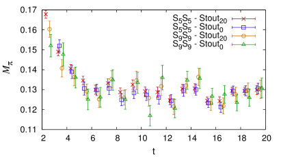
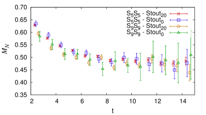
Throughout this paper, the notation $S_{i}S_{j}$ will be used to denote a calculation with source smearing $\sigma=i$ and sink smearing $\sigma=j$. Varying the parameter $N_{\rm GS}$ over the values shown in Table 2 did not impact any of the results, so it is dropped from further discussions. The notation V357 implies a $3\times 3$ variational analysis with $\sigma=3,\ 5,\ 7$.

In this paper we present a detailed analysis with two goals: First, to demonstrate that high precision estimates for the charges and the form-factors can be achieved cost effectively using the all-mode-averaging (AMA) method Blum et al. (2013). The second goal is to compare the 2-state fit to data at multiple $\mathop{t_{\rm sep}}\nolimits$ and variational methods Dragos et al. (2015) to determine the best strategy for controlling excited-state contamination in the matrix elements.

II.1 Lattice Parameters of the 4 Calculations

We analyze 4 high statistics simulations (labeled runs R1–R4) carried out on the $a081m312$ lattices. We explore the efficacy of using quark propagators with different smearing parameters to reduce the excited-state contamination and obtain estimates in the $t_{\rm sep}\to\infty$ limit. We compare three strategies for reducing excited-state contamination: optimizing the smearing parameters to reduce excited-state contamination in correlation functions; using the 2-state fit to correlation functions with data at multiple values of the source-sink separation $t_{\rm sep}$ (see Sec. II.3); and the variational method using a matrix of correlation functions constructed using up to three smearings as discussed in Sec. II.4. The lattice parameters used in these four runs are summarized in Table 2.

These four runs allow us to make four comparisons to understand, calculate and mitigate the excited-state contributions: (R1) a 2-state fit to data with smearing $\sigma=5$ and $t_{\rm sep}=10,12,14,16,18$; (R2) a variational calculation with a $3\times 3$ matrix of correlation functions constructed using $\sigma=3,5,7$ and $t_{\rm sep}=12\approx 1$ fm; (R3) a variational calculation with a $3\times 3$ matrix of correlation functions constructed using $\sigma=5,7,9$ and $t_{\rm sep}=12$; and (R4) a 2-state fit to data with smearing $\sigma=9$ and $t_{\rm sep}=10,12,14,16,18$. In the analysis of runs R2 and R3, we also present results from the three $2\times 2$ submatrices.

In each run, 96 low precision (LP) measurements were made on each of the 443 configurations that are separated by 10 RHMC trajectories. In three of the four runs (R1, R3 and R4), we also carried out 3 high precision (HP) measurements on each configuration to correct for possible bias in the LP calculation. As shown later, we find no significant indication of a bias in any of these three calculations, so we did not perform HP measurements in the case of R2 and give the mean values obtained from just the LP measurements as our final estimates.

ID	Method	Analysis	Smearing Parameters	$t_{\rm sep}$	LP	HP
R1	AMA	2-state	$\{5,60\}$	10,12,14,16,18	96	3
R2	LP	VAR	$\{3,22\}$, $\{5,60\}$, $\{7,118\}$	12	96
R3	AMA	VAR	$\{5,46\}$, $\{7,91\}$, $\{9,150\}$	12	96	3
R4	AMA	2-state	$\{9,150\}$	10,12,14,16,18	96	3

Table 2: Description of the four calculations (R1–R4) done to understand the dependence of the analysis on the smearing size $\sigma$, the efficacy of the variational method and the quality of the convergence of the 2-state fit using data at multiple source-sink separation $t_{\rm sep}$. The smearing parameters are $\{\sigma,N_{\rm GS}\}$ as described in the text. AMA indicates that the bias in the LP measurements was corrected using 3 HP measurements and Eq. (9). VAR indicates that the full $3\times 3$ matrix of correlation functions was calculated and a variational analysis performed as described in the text. Analysis using Eq. (7) to fit data at multiple $t_{\rm sep}$ simultaneously is labeled “2-state fit to data at multiple $t_{\rm sep}$ ”.

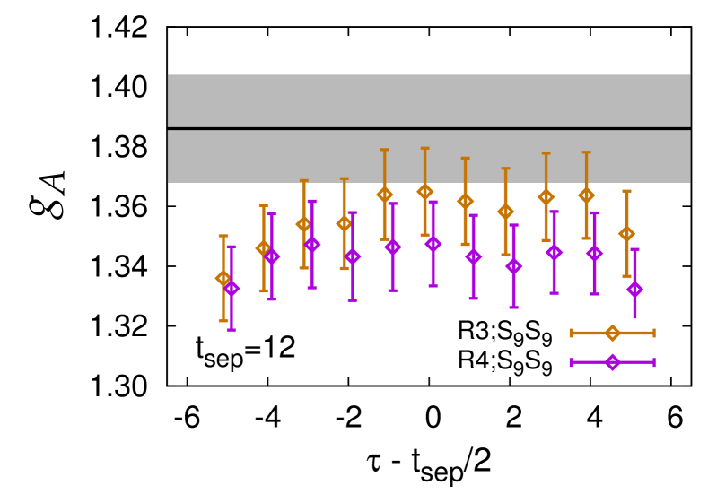
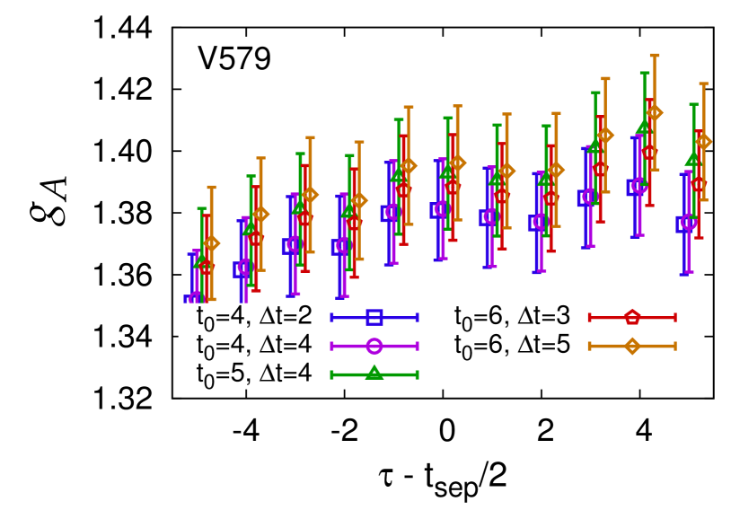
We caution the reader that some of the measurements have been made more than once in the different runs. The two calculations with smearing parameters $\{5,60\}$ (R1) and $\{5,60\}$ (part of R2) are identical. The two sets $\{5,60\}$ and $\{7,118\}$ (part of R2) and $\{5,46\}$ and $\{7,91\}$ (part of R3) differ in the number of iterations $N_{\rm GS}$ of the Klein-Gordon smearing operator and the choice of the location of the LP sources. Over the range investigated, we find that the results are insensitive to the value of $N_{\rm GS}$ and henceforth characterize the smearing by the single parameter $\sigma$. Different choices of the 96 randomly selected LP source positions on each configuration implies a different average over the gauge fields and the resulting difference provides a check on our estimation of the statistical errors. This is illustrated in Fig. 2 using data for $g_{A}$ with $\sigma=9$ and $t_{\rm sep}=12$ obtained from runs R3 and R4. Our final variational result V579 is also shown for comparison. We find that the difference in results from the two choices of LP source positions is comparable to our estimate of the statistical errors in the two measurements and the error in the V579 estimate, i.e., our estimation of errors is realistic.

Figure 2: Comparison of estimates of unrenormalized $g_{A}$ obtained with $\sigma=9$ and $t_{\rm sep}=12$ from the two different ‘ runs R3 and R4. The choice of the 96 LP source positions on each configuration is different in the two runs and the resulting difference in estimates is consistent with our estimate of statistical errors. The gray error band and the solid line within it is the V579 variational estimate discussed in the text.

II.2 Correlation Functions

The interpolating operator $\chi$ used to create and annihilate the nucleon state is

$$\chi(x)=\epsilon^{abc}\left[{q_{1}^{a}}^{T}(x)C\gamma_{5}\frac{(1\pm\gamma_{4})}{2}q_{2}^{b}(x)\right]q_{1}^{c}(x)$$ (1)

with color indices $\{a,b,c\}$, charge conjugation matrix $C=\gamma_{0}\gamma_{2}$, and the two different flavors of light quarks $q_{1}$ and $q_{2}$. The non-relativistic projection $(1\pm\gamma_{4})/2$ is inserted to improve the signal, with the plus and minus sign applied to the forward and backward propagation in Euclidean time, respectively.

The 2-point and 3-point nucleon correlation functions at zero momentum are defined as

$${\mathbf{C}}_{\alpha\beta}^{\text{2pt}}(t) =\sum_{\mathbf{x}}\langle 0|\chi_{\alpha}(t,\mathbf{x})\overline{\chi}_{\beta}(0,\mathbf{0})|0\rangle\,,$$ (2)

$${\mathbf{C}}_{\Gamma;\alpha\beta}^{\text{3pt}}(t,\tau) =\sum_{\mathbf{x},\mathbf{x^{\prime}}}\langle 0|\chi_{\alpha}(t,\mathbf{x})\mathcal{O}_{\Gamma}(\tau,\mathbf{x^{\prime}})\overline{\chi}_{\beta}(0,\mathbf{0})|0\rangle\,,$$ (3)

where $\alpha$ and $\beta$ are the spinor indices. The source time slice $t_{i}$ is translated to $t_{i}=0$; $t_{f}=t$ is the sink time slice; and $\tau$ is the time slice at which the bilinear operator $\mathcal{O}_{\Gamma}^{q}(x)=\bar{q}(x)\Gamma q(x)$ is inserted. The Dirac matrix $\Gamma$ is $1$, $\gamma_{4}$, $\gamma_{i}\gamma_{5}$ and $\gamma_{i}\gamma_{j}$ for scalar (S), vector (V), axial (A) and tensor (T) operators, respectively. Here, subscripts $i$ and $j$ on gamma matrices run over $\{1,2,3\}$, with $i<j$.

The charges $g_{\Gamma}^{q}$ in the nucleon state $|N(p,s)\rangle$ are defined as

$$\langle N(p,s)|\mathcal{O}_{\Gamma}^{q}|N(p,s)\rangle=g_{\Gamma}^{q}\bar{u}_{s}(p)\Gamma u_{s}(p)$$ (4)

with spinors satisfying

$$\sum_{s}u_{s}(\mathbf{p})\bar{u}_{s}(\mathbf{p})={\text{$\not\!p$}+m_{N}}\,.$$ (5)

To analyze the data, we construct the projected 2- and 3-point correlation functions

$$C^{\text{2pt}}(t) ={\langle\operatorname{Tr}[\mathcal{P}_{\text{2pt}}{\mathbf{C}}^{\text{2pt}}(t)]\rangle}$$

$$C_{\Gamma}^{\text{3pt}}(t,\tau) =\langle\operatorname{Tr}[\mathcal{P}_{\rm 3pt}{\mathbf{C}}_{\Gamma}^{\text{3pt}}(t,\tau)]\rangle\,.$$ (6)

The operator $\mathcal{P}_{\text{2pt}}=(1+\gamma_{4})/2$ is used to project on to the positive parity contribution for the nucleon propagating in the forward direction. For the connected 3-point contributions, $\mathcal{P}_{\rm 3pt}=\mathcal{P}_{\text{2pt}}(1+i\gamma_{5}\gamma_{3})$ is used. Note that the 3-point function in Eq. (6) becomes zero if $\Gamma$ anti-commutes with $\gamma_{4}$, so only $\Gamma=1$, $\gamma_{4}$, $\gamma_{i}\gamma_{5}$ and $\gamma_{i}\gamma_{j}$ elements of the Clifford algebra survive. To extract the charges, we make 2-state fits to the 2- and 3-point correlation functions defined in Eq. (6) as described next.

II.3 Behavior of the Correlation Functions

Our goal is to extract the matrix elements of the various bilinear quark operators between ground state nucleons. The lattice operator $\chi$, given in Eq. (1), couples not only to the nucleon but to all its excitations and multiparticle states with the same quantum numbers that are allowed on the lattice. The correlation functions, therefore, get contributions from all these intermediate states. Using spectral decomposition, the behavior of the 2- and 3-point functions is given by the expansion:

$$C^{\text{2pt}} (t_{f},t_{i})=$$

$${|{\cal A}_{0}|}^{2}e^{-M_{0}(t_{f}-t_{i})}+{|{\cal A}_{1}|}^{2}e^{-M_{1}(t_{f}-t_{i})}$$

$$+\ldots\,,$$

$$C^{\text{3pt}}_{\Gamma} (t_{f},\tau,t_{i})=$$

$$|{\cal A}_{0}|^{2}\langle 0|\mathcal{O}_{\Gamma}|0\rangle e^{-M_{0}t_{\rm sep}}+{}$$

$$|{\cal A}_{1}|^{2}\langle 1|\mathcal{O}_{\Gamma}|1\rangle e^{-M_{1}t_{\rm sep}}+{}$$

$${\cal A}_{0}{\cal A}_{1}^{*}\langle 0|\mathcal{O}_{\Gamma}|1\rangle e^{-M_{0}(\tau-t_{i})}e^{-M_{1}(t_{f}-\tau)}+{}$$

$${\cal A}_{0}^{*}{\cal A}_{1}\langle 1|\mathcal{O}_{\Gamma}|0\rangle e^{-M_{1}(\tau-t_{i})}e^{-M_{0}(t_{f}-\tau)}$$

$$+\ldots\,,$$ (7)

where we have shown all the contributions from the ground and one excited state. For simplicity, all the source positions are shifted to $t_{i}=0$, and in 3-point functions, the source-sink separation $t_{f}-t_{i}\equiv\mathop{t_{\rm sep}}\nolimits$. The states $|0\rangle$ and $|1\rangle$ represent the ground and “first” excited nucleon states, respectively. Throughout the paper it will be understood that, in practice, fits using Eq. (7) lump the contributions of all excited states into these two states, so demonstrating convergence of the estimates with respect to $t_{\rm sep}$ is important.

To extract the charges $g_{A}$, $g_{S}$, $g_{T}$ and $g_{V}$, we only need operator insertion at zero momentum, in which case ${\cal A}_{0}$ and ${\cal A}_{1}$ are real and the matrix element $\langle 0|\mathcal{O}_{\Gamma}|1\rangle=\langle 1|\mathcal{O}_{\Gamma}|0\rangle$. Thus, keeping one excited state in the analysis requires extracting seven parameters from fits to the 2- and 3-point functions. We use Eqs. (7) for the analysis of all the charges and form factors and call it the “2-state fit”.

Five of the seven parameters, $M_{0}$, $M_{1}$ and the three matrix elements $\langle 0|\mathcal{O}_{\Gamma}|0\rangle\equiv g_{\Gamma}$, $\langle 0|\mathcal{O}_{\Gamma}|1\rangle$ and $\langle 1|\mathcal{O}_{\Gamma}|1\rangle$ are physical provided the discretization errors and higher excited-state contaminations have been removed. The amplitudes ${\cal A}_{0}$ and ${\cal A}_{1}$ depend on the choice of the interpolating nucleon operator and/or the smearing parameters used to generate the smeared sources. It is evident from Eq. (7) that the ratio of the amplitudes, ${\cal A}_{1}/{\cal A}_{0}$, is the quantity to minimize in order to reduce excited-state contamination as it determines the relative size of the overlap of the nucleon operator with the first excited state.

We first estimate the four parameters, $M_{0}$, $M_{1}$, ${\cal A}_{0}$ and ${\cal A}_{1}$ from the 2-point function data and then use these as inputs in the extraction of matrix elements from fits to the 3-point data. Both of these fits, to 2- and 3-point data, are done within the same jackknife process to take into account the correlations between the errors. We performed both correlated and uncorrelated fits to the nucleon 2- and 3-point function data. In all cases in which the correlated fits were stable under changes in the fit ranges the two fits gave overlapping estimates. The final analysis of the 2-point function data used correlated $\chi^{2}$ fits. Since correlated fits to 3-point functions with multiple $t_{\rm sep}$ did not work in some cases, we used uncorrelated $\chi^{2}$ for 3-point fits for uniformity. The errors in both 2- and 3-point correlation functions have been calculated using a single elimination jackknife method.

To extract the three matrix elements $\langle 0|\mathcal{O}_{\Gamma}|0\rangle\equiv g_{\Gamma}$, $\langle 1|\mathcal{O}_{\Gamma}|0\rangle$ and $\langle 1|\mathcal{O}_{\Gamma}|1\rangle$ from the 3-point functions for each operator $\mathcal{O}_{\Gamma}=\mathcal{O}_{A,S,T,V}$ insertion, we make one overall fit using the data at all values of the operator insertion time $\tau$ and the various source-sink separations $t_{\rm sep}$ using Eq. (7). In practice, in all the fits, we neglect the data on the 3 points on either end, adjacent to the source and the sink, of the 3-point functions for each $t_{\rm sep}$ as they have the largest excited-state contamination. To the extent that the central values of $\tau$ dominate the 2-state fit, Eq. (7), to data at a single $\mathop{t_{\rm sep}}\nolimits$, the contributions of all higher states vanish in the limit $t_{\rm sep}\to\infty$. We extract this limit using the 2-state fit to data at multiple values of $\mathop{t_{\rm sep}}\nolimits$ in the range 0.8–1.4 fm. Also, as is evident from Eq. (7), the contribution of the matrix element $\langle 1|\mathcal{O}_{\Gamma}|1\rangle$ cannot be isolated from fits to 3-point function data obtained at a single finite value of $t_{\rm sep}$.

Post facto, using Eq. (7) and reliable estimates of $\langle 0|\mathcal{O}_{\Gamma}|1\rangle$, $\langle 1|\mathcal{O}_{\Gamma}|1\rangle$, the mass gap $M_{1}-M_{0}$, and the ratio ${\cal A}_{1}/{\cal A}_{0}$ one can bound the size of the excited-state contamination at central values of $\tau$ for a given source-sink separation $t_{\rm sep}$.

II.4 The variational Method

One can also reduce excited-state contamination by implementing a variational analysis (see Dragos et al. (2015) and references therein for previous use of the variational method for calculating nucleon matrix elements). This can be done by calculating 2-point and 3-point functions in two ways by (i) using a basis of nucleon interpolating operators with different overlap with the ground and excited states. The operator given in Eq. (1) is one such operator. (ii) Constructing multiple correlation functions with the same interpolating operator but defined with smeared quark fields using a number of different smearing sizes. In this work, we explore the second method in runs R2 and R3. In each of these two runs, the calculation is done using three different smearing parameters $S_{i}$ summarized in Table 2. The 2-point correlation function for the nucleon at each time $t$ is then a $3\times 3$ matrix, $G^{\rm 2pt}_{ij}(t)$, made up of correlation functions defined in Eqs. (2), (3) and (7) with source smearing $S_{i}$ and sink smearing $S_{j}$. The best overlap with the ground state is given by the eigenvector corresponding to the largest eigenvalue $\lambda_{0}$ obtained from the generalized eigenvalue relation Fox et al. (1982):

$$G^{\rm 2pt}(t+\Delta t)u_{i}=\lambda_{i}G^{\rm 2pt}(t)u_{i}\,,$$ (8)

where $u_{i}$ are the eigenvectors with eigenvalues $\lambda_{i}$. The matrix $G^{\rm 2pt}(t)$ at each $t$ should be symmetric up to statistical fluctuations, so we symmetrize it by averaging the off-diagonal matrix elements.

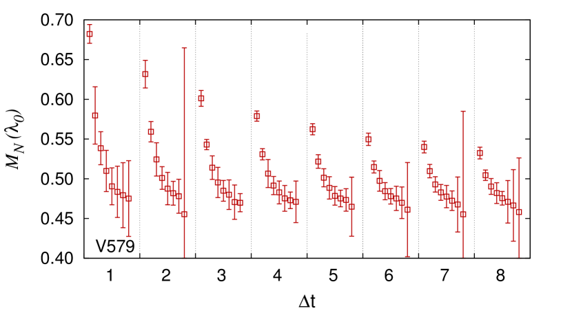
To select the $t$ and $\Delta t$ to use in the analysis, we show in Fig. 3 the nucleon mass $M_{N}(\lambda_{0})=-(\ln\lambda_{0})/\Delta t$ obtained from the ground state eigenvalue $\lambda_{0}$ for a range of combinations. The criteria we used for choosing the $t$ and $\Delta t$ used in the final analysis are: (i) the interval should be sensitive to both the ground and the excited states, (ii) the correlation functions should exhibit a good statistical signal over this range, (iii) the estimate of $M_{N}$ from $\lambda_{0}$ should be close to the final estimate of the ground state mass, and (iv) the resulting 2-state fit to the projected 2-point function should have a small value for the ratio ${\cal A}_{1}/{\cal A}_{0}$. Data in Fig. 3 show that $M_{N}$ starts to plateau towards its asymptotic value for $t\raisebox{-3.01385pt}{$\stackrel{{\scriptstyle\textstyle>}}{{\sim}}$ }5$ and the errors show a significant decrease for $\Delta t>2$. These trends still leave a number of “equally” good choices based on our four criteria, for example, $t=6$ and $\Delta t=3$ or $t=5$ and $\Delta t=4$. We selected $t=6$ and $\Delta t=3$.

Figure 3: Estimates of the nucleon mass from the largest eigenvalue of the $3\times 3$ matrix V579 as a function of $t$ and $\Delta t$. For clarity, the vertical dashed lines separate the sets of eight ($t=1-8$) estimates for a given value of $\Delta t$. Data show that the asymptotic estimate $M_{0}\approx 0.47$ given in Table 4 is reached only for $t>5$ and there is a significant decrease in the errors for $\Delta t>2$.

Figure 4: Nucleon effective mass at zero momentum as a function of Euclidean time $t$. (Top) Results for smearing size $\sigma=3,5,7,9$; (Middle) comparison of $\sigma=3,5,7$ single smearing data with the variational data V357; and (Bottom) comparison of $\sigma=5,7,9$ single smearing data with the variational data V579.

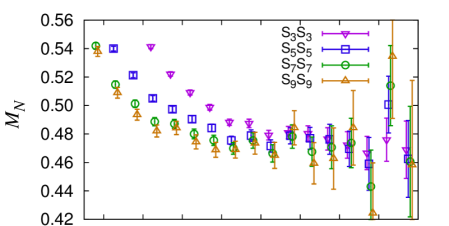
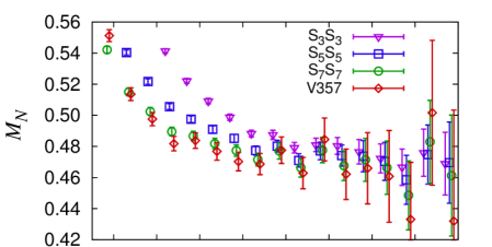
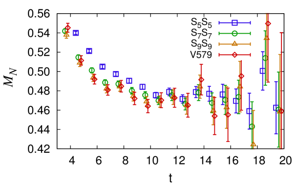
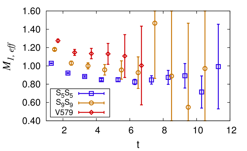
With a good estimate of $u_{0}$, the expectation is that the ground state, in the projected functions $u_{0}^{T}G^{\rm 2pt}(t)u_{0}$ dominates at earlier $t$. In Fig. 4, we compare the behavior of the nucleon effective mass obtained from correlation functions with different smearing and with the projected variational V357 and V579 data. We find that as the smearing size $\sigma$ is increased, the plateau sets in at earlier time (top panel). The V357 data are a little below $S_{7}S_{7}$ (middle panel) while V579 overlap with $S_{9}S_{9}$ (bottom panel). In Fig. 5, we compare the effective mass plot for the excited state, i.e., that obtained by subtracting the ground state result from the nucleon correlation function. Estimates of $M_{1}$ increase from $S_{5}S_{5}$ to $S_{9}S_{9}$ to V579, indicating that the contribution of higher excited states becomes larger as more of the first excited state is removed. Also, the excited state signal in V579 dies out by $t\approx 8$. This behavior of $M_{1}$ informed our choice $t=6$ and $\Delta t=3$ with which we estimated the eigenvectors $u_{i}$.

Figure 5: Plot of the effective mass for the excited state evaluated from the $S_{5}S_{5}$, $S_{9}S_{9}$ and V579 nucleon correlation functions after subtraction of the respective ground state fit.

Figure 6: Estimates of the unrenormalized $g_{A}$ from the V579 analysis for five representative values of $t$ and $\Delta t$ used to diagonalize the $3\times 3$ 2-point matrix correlation function and obtain the eigenvector used in the diagonalization of the 3-point correlation matrix. All final results are obtained with the choice $t=6$ and $\Delta t=3$.

Similarly, in the variational analysis for the 3-point functions $C^{\rm 3pt}(\tau,t_{\rm sep})$, from which various charges are extracted, the data at each $\tau$ and $\mathop{t_{\rm sep}}\nolimits$ are $3\times 3$ matrices. The ground state estimate is obtained by projecting these matrices $G^{\rm 3pt}$ using the $u_{0}$ estimated from the 2-point variational analysis, Eq. (8), i.e., $u_{0}^{T}G^{\rm 3pt}(\tau,t_{\rm sep})u_{0}$. We use the eigenvectors determined with $t=6$ and $\Delta t=3$ for projecting the 3-point data at all $\tau$. These projected data define the variational 3-point function that is then fit using the 2-state ansatz given in Eq. (7), but with the $\langle 1|\mathcal{O}_{\Gamma}|1\rangle$ term set to zero, to obtain the charges. Note that the eigenvectors $u_{i}$ do not depend on $t_{\rm sep}$. Also, we use the same $u_{0}$ for all $\tau$.

To understand the sensitivity of this projected 3-point data to our choice $t=6$ and $\Delta t=3$ for estimating $u_{0}$, we show $g_{A}$ data for 5 representative combinations, that satisfy our selection criteria, in Fig. 6. We find that all five give estimates are consistent and have errors of roughly the same size. Estimates from the combination $\{t,\Delta t\}=\{4,2\}$ and $\{4,4\}$ are about $0.5\sigma$ below the other three, $\{5,4\}$, $\{6,3\}$ and $\{6,5\}$. We consider the latter three to be equally good choices.

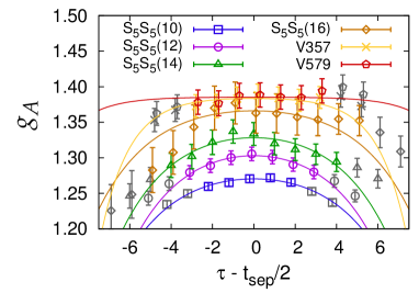
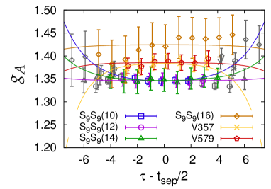
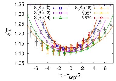
In the variational analysis carried out using data at a single $t_{\rm sep}$, the signal for a reduction in the excited-state contamination in the projected correlation function is a larger flatter plateau, i.e., it should show less dependence on the operator insertion time $\tau$ compared to a correlation function with the same $t_{\rm sep}$ but with a single smeared source. We illustrate this feature using the data from R2 for $g_{A}$ in Fig. 14. The four variational estimates have a larger plateau and a larger value compared to $S_{5}S_{5}$ with $t_{\rm sep}=12$. This improvement is less obvious when comparing V579 to the $S_{9}S_{9}$ data because, as discussed in Sec. IV, $S_{9}S_{9}$ has much smaller contributions from the excited states and has a plateau comparable in extent to V579.

If $\langle 0|\mathcal{O}_{\Gamma}|1\rangle$ is the dominant contamination, one can also set up and solve an optimization condition using the $3\times 3$ matrix of 3-point data $M(\tau)\equiv\operatorname{Tr}[{\cal P}_{\Gamma}C_{\Gamma}^{\rm 3pt}(t_{\rm sep},\tau)]$. In this case, one needs to determine the projection vector $\zeta$ such that $\zeta^{T}M(\tau)\zeta$ is insensitive to $\tau$. Again, to be sensitive to excited states in the determination of $\zeta$, one needs to choose $\tau$ in a region where the excited-state effect is significant. Also, a good estimate of $\zeta$ should make the projected correlation function flatter. This analysis, in general, needs to be done separately for each charge. We have not carried out this more elaborate analysis.

II.5 Test of the coherent sequential source method

The coherent sequential source method is a technique to reduce computational cost in the connected 3-point functions Bratt et al. (2010). It relies on the observation that for a large enough lattice independent measurements can be made using a distributed array of sources. Then, instead of calculating a separate sequential propagator from each sink, a single coherent sequential propagator may be calculated from the sum of all the sink source points.

In our calculations on the $a081m312$ lattices, the signal in the nucleon 2-point function becomes poor for $t>16$ as shown in Fig. 4. We, therefore, partition the lattice with Euclidean time extent $T=64$ into three sublattices of length $21$ ($(T/3)_{\rm int}$) Yamazaki et al. (2009). We calculate the 2- and 3-point functions on the three sublattices of a given lattice in a single computer job. We start by calculating three quark propagators from randomly selected source positions on the time slices $t_{i}=r,\ r+21$ and $r+42$, where $r\in\{1-21\}$. (To decrease correlations, $r$ is offset by 9 time slices between successive configurations). The three measurements of the 2-point functions are made using these three independently calculated propagators. The calculation of the 3-point functions is done by inserting a zero-momentum nucleon state at Euclidean times $t_{f}=t_{i}+t_{\rm sep}$ using these propagators and the interpolating operator given in Eq. (1). These nucleon states at the three sink time slices $t_{f}$ have uncontracted spin and color indices, associated with either the $u$ or the $d$ quark in the nucleon interpolating operator. These states are used as sources to generate the corresponding $u$ and $d$ sequential propagators. An illustration of the construction of these three sources in different parts of the lattice is shown in Fig. 7.

Figure 7: Illustration of the construction of the sequential sources, $u_{i}$, for each spin and color component of the $u$ quark in three well-separated regions of the lattice. The insertion of the neutron at each of the three sink time slices $t_{f}$ is done using quark propagators $P_{i}$ generated independently from three initial time slices $t_{i}$. The three sources, $u_{i}^{\rm seq}$, are then added to produce the coherent sequential source.

Figure 8: Illustration of the construction of the 3-point function in the first of the three regions using the coherent sequential source propagator, $P^{\rm seq}$. The original propagator, $P$, from the source $u$ at $t_{i}^{1}$ is contracted with the quark bilinear operator at an intermediate time $\tau$ marked with a cross and $P^{\rm seq}$ from the sequential source $u$ at $t_{f}^{1}$. The contributions of the other two sources to $P^{\rm seq}$ are shown by the black dotted lines and average to zero by gauge invariance because the 3 sources are not connected by either gauge links or quark lines.

To obtain the 3-point function, this sequential propagator from $t_{f}=t_{i}+t_{\rm sep}$ and the original propagator from $t_{i}$ are then contracted with the operator at all intermediate time slices $\tau$ between $t_{i}$ and $t_{f}$ using Eq. (6).

In the coherent sequential source method the three regions of the lattice are regarded as independent. Under this assumption, the three $u$ ($d$) sources with nucleon insertion at $r+t_{\rm sep}$, $r+21+t_{\rm sep}$ and $r+42+t_{\rm sep}$ can be added before the inversion for creating the sequential $u$ ($d$) propagators, respectively. Such a summed source is called a coherent source Bratt et al. (2010) and using it reduces the computational cost from $N_{\rm meas}+2\times N_{\rm meas}$ to $N_{\rm meas}+2$ inversions when $N_{\rm meas}$ measurements are done at the same time on different parts of the lattice.

The contributions of a coherent source in the region, say $r\leq t\leq r+t_{\rm sep}$, is illustrated in Fig. 8. The contributions from the other two sources, shown by dotted lines, to gauge invariant correlation functions are formally zero on gauge averaging, however, they can increase the statistical fluctuations. Therefore, one has to demonstrate that for a finite statistical sample, the extra noise introduced is small so that there is an overall reduction in computational cost. The magnitude of the noise, for fixed statistics, is reduced by increasing the distance between the sources, which we accomplish by choosing $N_{\rm meas}=3$ partitions on a lattice with $T=64$.

To validate the assumption that with our coherent source construction and finite statistics, the measurements in the region, for example, $r\leq t\leq r+t_{\rm sep}$ do not have significantly enhanced errors due to contributions from the nucleon sources at $r+21+t_{\rm sep}$ and $r+42+t_{\rm sep}$, i.e., their contribution averages to zero and there is no significant increase in the error estimates, we simulated 100 configurations with the same parameters and source/sink locations as Run 4 but without using the coherent source trick. The data for the four charges, summarized in Table 3, show that (i) the difference in the mean values for the 3-point function data, averaged over these 100 configurations, is smaller than the statistical errors in all cases and (ii) there is no significant difference in the error estimates with the coherent source trick. Parenthetically, we remark that in the case of correlation functions at large momenta (needed for the form factor calculations), the differences in the means are as large as $30\%$, however, the statistical errors in these data are $O(1)$. Note that any difference or any additional noise in any of the correlation functions due to the coherent source trick is even smaller in our final analysis with the full set of 443 configurations.

Analysis	$g_{A}$	$g_{S}$	$g_{T}$	$g_{V}$
Coherent	1.368(50)	1.34(23)	1.132(44)	1.217(32)
No Coherent	1.377(47)	1.33(25)	1.138(44)	1.199(33)

Table 3: Comparison of estimates for the four charges with and without the coherent sequential source trick using the $S_{9}S_{9}$ setup with a subset of 100 configurations.

Our overall conclusion is that with a judicious partitioning of the lattice with a large $T$ extent, the coherent sequential source method does not give rise to a detectable increase in the statistical errors for the charges. The reduction in the computational cost is significant: it reduces the number of inversions from $N_{\rm meas}+2\times N_{t_{\rm sep}}\times N_{\rm meas}$ to $N_{\rm meas}+2\times N_{t_{\rm sep}}$, which for $N_{\rm meas}=3$ and $N_{t_{\rm sep}}=5$ is a reduction by a factor of 2.5.

II.6 The AMA Method for High Statistics

To increase the statistics, given a fixed number of configurations, the calculation was carried out using the all-mode-averaging (AMA) technique Blum et al. (2013) with $96$ low precision (LP) and $3$ high precision (HP) measurements, respectively. Also, the calculations used the coherent sequential source method discussed in Sec. II.5 to reduce the computational cost. To implement these methods, we carried out three measurements on a given configuration at the same time. As discussed in Sec. II.5, the three starting source points were placed on three time slices $t_{i}=r$, $r+21$ and $r+42$ and offset by 9 time slices between successive configurations to improve decorrelations.

The locations of the 32 LP source points on each of these three time slices $t_{i}$ were selected as follows to reduce correlations: the first point was selected randomly and the remaining 31 points were offset by multiples of $N_{x}=16$, $N_{y}=8$ and $N_{z}=8$. The resulting 96 LP estimates for 2- and 3-point functions from these sources are, a priori, biased since the Dirac matrix is inverted with a low precision stopping criterion. To remove this bias, we place an additional high precision (HP) source on each of the 3 time slices from which we calculate both LP and HP correlation functions. Thus, in our implementation of the AMA method, $93+3$ LP and 3 HP measurements were done on each configuration for runs R1, R3 and R4. In R2, no HP measurements were made and the results are averages over the 96 LP measurements.

Using HP and LP correlators on each configuration, the bias corrected 2- and 3- point functions are given by

$$C^{\text{AMA}} =\frac{1}{N_{\text{LP}}}\sum_{i=1}^{N_{\text{LP}}}C_{\text{LP}}(\mathbf{x}_{i}^{\text{LP}})$$

$$+ \frac{1}{N_{\text{HP}}}\sum_{i=1}^{N_{\text{HP}}}\left[C_{\text{HP}}(\mathbf{x}_{i}^{\text{HP}})-C_{\text{LP}}(\mathbf{x}_{i}^{\text{HP}})\right]\,,$$ (9)

where $C_{\text{LP}}$ and $C_{\text{HP}}$ are the correlation functions calculated in LP and HP, respectively, and $\mathbf{x}_{i}^{\text{LP}}$ and $\mathbf{x}_{i}^{\text{HP}}$ are the two kinds of source positions. The bias in the LP calculation (first term) is corrected by the second term provided the correlation functions are translationally invariant, which the 2- and 3-point functions are. If the algorithm used to invert the Dirac matrix handles all modes well, $i.e.$ the HP and LP calculations from the same source point are correlated, then the error in the AMA estimate is dominated by the LP measurement and the bias correction term does not significantly increase the error.

We used the multigrid algorithm for inverting the Dirac matrix Babich et al. (2010) and set the low-accuracy stopping criterion $r_{\rm LP}\equiv|{\rm residue}|_{\rm LP}/|{\rm source}|=10^{-3}$ and the HP criterion to $r_{\rm HP}=10^{-10}$. To quantify the bias, we have compared the AMA and LP estimates for both the 2- and 3-point correlation functions themselves and for the seven fit parameters $M_{0}$, $M_{1}$, ${\cal A}_{0}$, ${\cal A}_{1}$, $\langle 0|\mathcal{O}_{\Gamma}|0\rangle$, $\langle 0|\mathcal{O}_{\Gamma}|1\rangle$ and $\langle 1|\mathcal{O}_{\Gamma}1\rangle$. In each case we find that the difference between the two is a tiny fraction (few percent) of the statistical error in either.

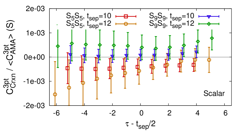
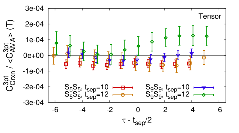
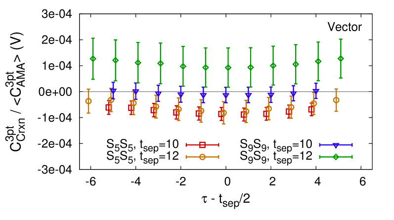
We illustrate the size and behavior of the bias correction term in the pion and nucleon 2-point correlators as a ratio to the signal in Fig. 9. In the case of the nucleon 2-point function we find that the bias correction term is $\raisebox{-3.01385pt}{$\stackrel{{\scriptstyle\textstyle<}}{{\sim}}$ }10^{-4}$ of the signal for all $t$. In the case of the pion 2-pt function, which has the smallest errors and whose signal does not degrade with $t$, the correction term grows with $t$ but remains $<10^{-3}$ for $t<25$. In Fig. 10, we show the data for the four charges. In the cases of $g_{A}$, $g_{T}$ and $g_{V}$, the effect is again $O(10^{-4})$. It is $O(10^{-3})$ for $g_{S}$ but in this case the statistical errors are also correspondingly larger. In Table 5, we show that the results for the unrenormalized charges with and without the bias correction term are essentially identical. Based on such comparisons that have been carried out for all the correlation functions, we conclude that any possible bias in the LP calculations is negligible compared to our current statistical errors.

Figure 9: The ratio of the bias correction term defined in Eq. (9) to the AMA correlator as a function of Euclidean time $t$ for (left) the pion and (right) nucleon 2-point functions. The data are from runs R1 and R4 with $S_{5}S_{5}$ and $S_{9}S_{9}$, respectively.

Figure 10: The ratio of the bias correction term defined in Eq. (9) to the AMA correlator as a function of operator insertion time $\tau$ for the four charges. We show data from both runs R1 and R4.

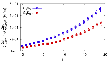
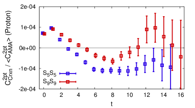
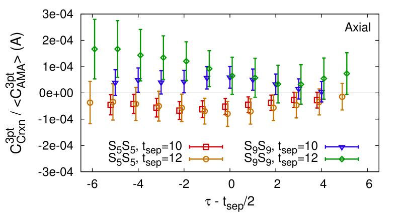
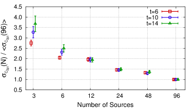
In current lattice QCD simulations of nucleon charges and form factors, the most computationally expensive part is the generation of lattices. Thus one wants to extract the most precise results from a fixed number of gauge configurations by having a large number of LP measurements on each configuration. To consider the cost effectiveness of the AMA method, we use the data presented in this work to compare the decrease in errors with 96 LP + 3 HP measurements versus 35 HP measurements. These two calculations have the same computational cost on these lattices because one HP measurement takes the same time as three LP ones. As discussed above, since there is no detectable difference in the values or errors between LP and HP measurements, we, therefore, use the more extensive LP data to make this comparison. In Fig. 11, we show the decrease in errors with the number of LP measurements made on each gauge configuration for both the 2-point nucleon correlation function and the four charges. These errors were calculated by first averaging over randomly selected 3, 6, 12, 24 or 48 of the 96 measurements on each configuration and then performing a jackknife analysis over the 443 configurations. We find that the errors decrease by $\approx 1.4$ between LP=35 and 96, i.e., a gain in statistics by a factor of 2. The continued reduction in errors up to $96$ LP measurements is what gives a factor of 2 saving with the 96 LP + 3 HP over 35 HP measurements. This, post facto, justifies using $O(100)$ measurements on each configuration. In a related study Bhattacharya et al. (2016), we found that at the physical pion mass, one HP measurement costs as much as 17 LP ones with the multigrid inverter. Thus, the cost effectiveness of the AMA method increases very significantly as the light quark masses are lowered towards their physical value.

Figure 11: (Left) The reduction in errors in the nucleon 2-point correlator as a function of the number of LP sources averaged per configuration. The data are shown for three different source-sink separations $t=6,10,14$. (Right) The ratio of errors in the four unrenormalized charges as a function on the number of LP sources analyzed. The data are from run R4 with $S_{9}S_{9}$. The data shown are at the midpoint $\tau=5$ of the $t_{\rm sep}=10$ calculation. In both figures, the error estimates from $N$ LP measurements are normalized by those from 96 LP measurements.

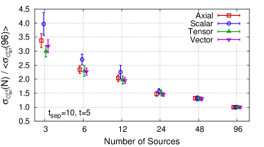
Lastly, as discussed earlier, a second feature we incorporate in the AMA calculation to improve statistical precision by reducing correlations between measurements is to choose the source points randomly within and between configurations.

Our conclusion is that already on $M_{\pi}=300$ MeV lattices, the AMA method is a cost effective way to increase the statistics. Our results suggest a stronger statement for the calculation of nucleon charges and form factors: with an inverter such as multigrid that does not exhibit critical slowing down and becomes more efficient as the quark mass is reduced, using $r_{\rm LP}=10^{-3}$ as the stopping criteria does not give rise to any significant bias compared to the statistical errors estimated from $O(100,000)$ measurements. The LP measurement should, therefore, be considered unbiased at this level of statistical precision and performing $O(100)$ measurements per configuration is cost effective.

III Statistical Errors

In this section, we study the size of errors in 2- and 3-point correlation functions as a function of the smearing size $\sigma$ and the source-sink separation $t_{\rm sep}$ and compare them to those in the variational estimates.

III.1 Statistical Errors in 2-point Functions

The nucleon 2-point correlation function was calculated 8 times over the course of the four runs. The resulting values of the two masses $M_{0}$ and $M_{1}$ and the amplitudes ${\cal A}_{0}$ and ${\cal A}_{1}$ are given in Table 4 along with the fit range $t_{\rm min}-t_{\rm max}$. All the estimates for $M_{0}$ are consistent within errors. Note that the two sets of $S_{5}S_{5}$ and $S_{7}S_{7}$ measurements from runs R2 and R3 are different because different LP source positions were used, i.e., the average over gauge field fluctuations is different. In both cases we find that the difference in the estimates is smaller than the quoted statistical errors in either measurement.

Type	Fit Range	$aM_{0}$	$aM_{1}$	${\cal A}_{0}^{2}$	${\cal A}_{1}^{2}$	${\cal A}_{1}^{2}/{\cal A}_{0}^{2}$	$\chi^{2}/{\rm d.o.f.}$
$S_{5}S_{5}$	4–15	0.4717(38)	0.850(40)	2.85(13)e-08	3.45(19)e-08	1.212(59)	0.86
$S_{3}S_{3}$	6–20	0.4720(50)	0.844(41)	6.01(41)e-07	1.54(17)e-06	2.57(19)	0.79
$S_{5}S_{5}$	4–15	0.4717(38)	0.850(40)	2.85(13)e-08	3.45(19)e-08	1.211(59)	0.86
$S_{7}S_{7}$	4–15	0.4696(44)	0.855(83)	5.50(30)e-12	4.14(53)e-10	0.752(78)	0.60
V357	2–14	0.4736(25)	1.194(47)	6.43(14)e-11	9.82(61)e-11	1.526(81)	0.59
$S_{5}S_{5}$	4–15	0.4709(40)	0.849(40)	2.80(14)e-08	3.41(18)e-08	1.219(60)	0.99
$S_{7}S_{7}$	4–15	0.4683(46)	0.854(83)	5.38(31)e-12	4.14(52)e-10	0.769(77)	0.67
$S_{9}S_{9}$	3–15	0.4700(32)	1.031(84)	4.70(15)e-12	4.48(66)e-12	0.95(12)	0.60
V579	2–14	0.4710(27)	1.148(55)	1.316(32)e-12	1.73(13)e-12	1.316(83)	0.60
$S_{9}S_{9}$	4–15	0.4652(52)	0.87(12)	4.42(29)e-12	3.25(73)e-12	0.74(13)	0.81
$S_{9}S_{9}$	3–15	0.4682(35)	0.986(83)	4.59(17)e-12	4.27(57)e-12	0.93(10)	0.84
$S_{9}S_{9}$	2–15	0.4701(27)	1.061(48)	4.70(12)e-12	4.93(27)e-12	1.05(5)	0.88

Table 4: Estimates of the masses $M_{0}$ and $M_{1}$ and the amplitudes ${\cal A}_{0}$ and ${\cal A}_{1}$ extracted from the fits to the 2-point correlation functions using the 2-state ansatz given in (7) and using the variational method. The data are organized by the four separate runs described in the text and Table 2. The notation $S_{3}S_{3}$ labels a nucleon correlation function with source and sink constructed using smearing parameter $\sigma=3$. V357 stands for a $3\times 3$ variational analysis with smearings $\sigma=3,5,7$. We also give the $\chi^{2}/{\rm d.o.f.}$ for these fits obtained using the full covariance matrix. For $S_{9}S_{9}$ from R4, we give results with three different fit ranges to show sensitivity to $t_{\rm min}$.

In Fig. 4, we compare the estimates for the effective mass, $M_{N,eff}(t+0.5)=\ln(C^{\rm 2pt}(t)/C^{\rm 2pt}(t+1))$, obtained from runs with different smearing parameters and with the variational estimates. Together with the results given in Table 4, we note that

• the excited-state contamination decreases with $\sigma$ over the range studied and the plateau sets in at earlier time slices, however, the errors in the data increase with $\sigma$.

• The V357 estimate of $M_{N,{\rm eff}}$ lies below $S_{7}S_{7}$ data and the V579 values overlap with the $S_{9}S_{9}$ data. The errors in the V357 variational data shown in Fig. 4 are larger than in $S_{7}S_{7}$ but the results of the fits shown in Table 4 have smaller errors. The same is true for V579 versus the $S_{9}S_{9}$ data. This is because, to get the final estimates, the V357 and V579 data are fit with a smaller $t_{\rm min}$ as shown in Table 4.

• Estimates of $M_{0}$, using the 2-state fit and the variational analysis, agree within errors in all cases as shown in Table 4.

• Estimates of $M_{1}$ from the individual 2-state fits agree, however, the variational ansatz gives a significantly larger value. This feature is found to be independent of our choice of $t$ and $\Delta t$ in the construction of the variational ansätze. This is because the estimates are being extracted with a smaller $t_{\rm min}$, so the contributions of the higher states are larger. One can see a similar behavior in the $S_{9}S_{9}$ estimates shown for three different fit ranges in Table 4. Also note that the errors in estimates from fits with a smaller $t_{\rm min}$ are smaller.

• The ratio ${\cal A}_{1}^{2}/{\cal A}_{0}^{2}$, reducing which reduces the excited-state contamination, is found to decrease on increasing the smearing size from $\sigma=3$ to $\sigma=7$. Our estimate for $S_{9}S_{9}$ with our best fit-range 3—15 is larger than that for $S_{7}S_{7}$, but on using a common fit range, $4-15$, one finds a leveling off for $\sigma\raisebox{-3.01385pt}{$\stackrel{{\scriptstyle\textstyle>}}{{\sim}}$ }7$. This stabilization leads us to conclude that $\sigma\approx 7$, or $\sigma\approx 0.57$ fm in physical units, is the best compromise choice between reducing the ratio ${\cal A}_{1}/{\cal A}_{0}$ and keeping the statistical errors small.

• Two-state fits to the variational correlation functions are done with an earlier starting time slice, as they have little sensitivity to the excited-states beyond $t=6$ and become unstable for $t_{\rm min}\raisebox{-3.01385pt}{$\stackrel{{\scriptstyle\textstyle>}}{{\sim}}$ }4$. Comparing the two variational runs, we note that the ratio ${\cal A}_{1}^{2}/{\cal A}_{0}^{2}$ for V579 is smaller than for V357, similar to the trend seen in the 2-state fit.

• The data in Table 4 show that ${\cal A}_{1}^{2}/{\cal A}_{0}^{2}$ increases as $t_{\rm min}$ is decreased. While, this pattern is clear for each method, it is not obvious how to compare the values between methods. Even for the same fit range, the value from the variational method is significantly larger than that from the single smearing 2-state fit even though the data suggest that the overall excited state contamination in $M_{0}$ and the charges is smaller. The most likely explanation is that the contributions of higher states is larger at small $t$ but these die off faster due to their larger masses.

The bottom line is that the errors in $M_{0}$, $M_{1}$, ${\cal A}_{0}$ and ${\cal A}_{1}$ shown in Table 4 are sensitive to the fit range, which in turn depends on $\sigma$. As the excited-state contamination is reduced, fits can be made with an earlier starting time $t_{\rm min}$ and the errors in $M_{0}$ and $M_{1}$ become smaller. However, with a smaller $t_{\rm min}$, the estimated $M_{1}$ and the ratio of amplitudes ${\cal A}_{1}^{2}/{\cal A}_{0}^{2}$ is larger, most likely due to the larger contribution of the higher excited states at short Euclidean times. To get estimates for $M_{1}$ and ${\cal A}_{1}$ that are insensitive to the fit range will require much more precise data to which a 3-state fit can be made.

III.2 Statistical Errors in the 3-point Functions

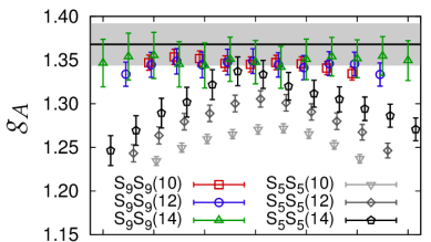
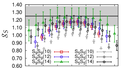
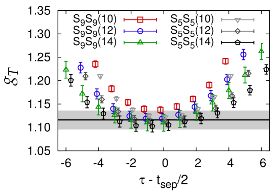
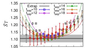
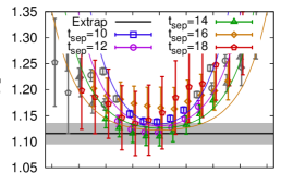
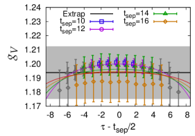
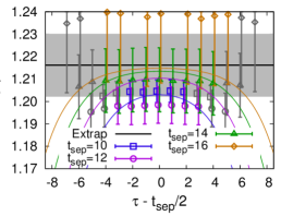
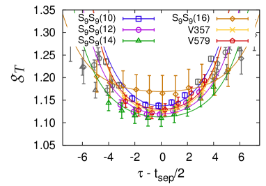
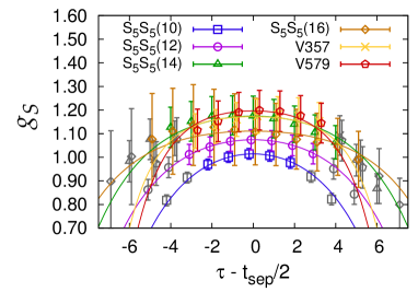
The errors in the charges are a combination of the statistical errors in the data for the correlation functions and the uncertainty in the fits used ($n-$state, fit-range, $\cdots$) to extract the matrix elements. This is true in both methods: the 2-state fit and the variational analysis. To exhibit the behavior of the charges as a function of $\mathop{t_{\rm sep}}\nolimits$ and $\tau$, we show in Fig. 12, and in all similar figures henceforth, the data for the 3-point function divided by the result of the 2-point fit, ${\cal A}_{0}^{2}\exp{(-M_{0}\mathop{t_{\rm sep}}\nolimits)}+{\cal A}_{1}^{2}\exp{(-M_{1}\mathop{t_{\rm sep}}\nolimits)}$. This construction of the “ratio” plot is a variant of the standard method in which the data for the 2-point function at appropriate $\mathop{t_{\rm sep}}\nolimits$, and not the result of the fit, are used for the normalization.

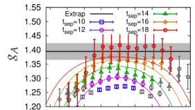
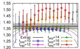
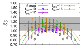
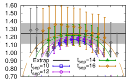
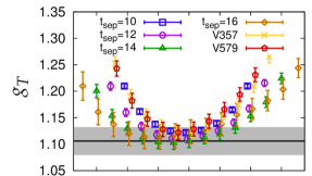
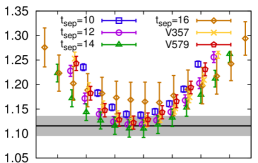
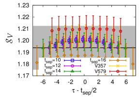
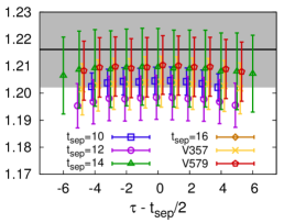
In Fig. 12, we compare the $t_{\rm sep}=10,12,14$ data for the isovector charges between R1 ($\sigma=5$) and R4 ($\sigma=9$) runs. We find that the excited-state contamination in $g_{A}$ and $g_{S}$ is significantly reduced in the data with $\sigma=9$, however, the errors are about 50% larger on each $t_{\rm sep}$ when compared to the $\sigma=5$ data. In the case of $g_{T}$, the excited-state contamination at central values of $\tau$ is smaller than $5\%$ in both cases with the $\sigma=5$ data showing a slightly smaller effect and smaller statistical errors. The data also show that the statistical errors increase by about $80\%$ for every two units of $t_{\rm sep}$. To first approximation, this holds for all four charges and for both smearing sizes. Thus, to reduce computational cost, the goal is to tune methods to get the $t_{\rm sep}\to\infty$ estimate from simulations with the smallest $t_{\rm sep}$.

In Fig. 13, we extend this comparison to include the results of the 2-state fit. We find that the two $t_{\rm sep}\to\infty$ estimates, $S_{5}S_{5}$ and $S_{9}S_{9}$, overlap for all four charges, and the final error estimates are comparable even though the errors in the 3-point data $C^{\rm 3pt}(\tau,\mathop{t_{\rm sep}}\nolimits)$ for $S_{9}S_{9}$ are larger. Based on the observation that the 2-state fit to the $S_{5}S_{5}$ data gives a reliable $t_{\rm sep}\to\infty$ estimate even though the excited-state contamination is significant whereas the $S_{9}S_{9}$ data show much smaller excited-state contamination but the fit is less reliable as the data overlap and have larger errors, we again conclude that $\sigma\approx 7$ is the best compromise choice for reducing the excited-state contamination in these charges and having small enough errors in the data at different $\mathop{t_{\rm sep}}\nolimits$ to give confidence in a 2-state fit. To improve the estimates from such 2-state fits, the statistical errors in the larger $t_{\rm sep}$ data need to be reduced.

Figure 12: Ratio plot comparing the statistical errors and excited-state contamination in the three unrenormalized isovector charges between runs R1 ($S_{5}S_{5}$) and R4 ($S_{9}S_{9}$) for values of $t_{\rm sep}=10,12,14$ shown within parenthesis. The error band and the solid line within it are the $t_{\rm sep}\to\infty$ results of fits to the $S_{9}S_{9}$ data. In most cases, the data with the two different smearings start to overlap by $t_{\rm sep}=14$. The errors in the data with $t_{\rm sep}=16$, shown in Fig. 13, are too large to confirm the convergence.

Figure 13: Data and fits for the unrenormalized isovector charges from runs R1 with $\sigma=5$ (left) and R4 $\sigma=9$ (right). In each case, the gray band and the solid line within it is the $t_{\rm sep}\to\infty$ estimate obtained using the 2-state fit. The $S_{5}S_{5}$ fit used the $t_{\rm sep}=[12,14,16,18]$ data while the $S_{9}S_{9}$ fit used the $t_{\rm sep}=[10,12,14,16]$ data. To significantly improve the 2-state fit to $S_{9}S_{9}$ requires at least doubling the statistics to reduce errors in the $t_{\rm sep}=16$ and $18$ data.

IV Excited-State Contamination

The overall goal is to get the best $t_{\rm sep}\to\infty$ estimates on each ensemble for a given computational cost. In this Section, we investigate the efficacy of using different smearing parameters, the 2-state fit with data at multiple $t_{\rm sep}$ and a variational analysis towards this goal. The final results for the charges are given in Table 5. The overall observation is that for each of the four charges, all four estimates agree within $1\sigma$, however, the errors in the estimates from the variational analysis V357 (V579) are about $60\%$ ($35\%$) smaller than those from $S_{5}S_{5}$ ($S_{9}S_{9}$), respectively.

Analysis	$g_{A}$	$g_{S}$	$g_{T}$	$g_{V}$
$S_{5}S_{5}$	1.395(29)	1.15(15)	1.106(26)	1.194(19)
$S_{5}S_{5}$*	1.395(29)	1.15(15)	1.106(26)	1.194(19)
$S_{9}S_{9}$	1.368(24)	1.25(13)	1.116(20)	1.216(14)
$S_{9}S_{9}$*	1.369(24)	1.25(13)	1.116(20)	1.216(14)
V35	1.365(13)	1.173(60)	1.123(10)	1.213(8)
V37	1.375(15)	1.183(66)	1.114(11)	1.206(8)
V57	1.381(16)	1.189(70)	1.112(12)	1.204(9)
V357	1.386(16)	1.185(75)	1.116(13)	1.205(10)
V57	1.373(16)	1.166(78)	1.108(13)	1.207(10)
V59	1.382(17)	1.202(84)	1.113(14)	1.209(10)
V79	1.385(18)	1.214(86)	1.115(15)	1.210(11)
V579	1.386(18)	1.220(87)	1.116(15)	1.210(11)
V579*	1.386(18)	1.220(87)	1.116(15)	1.210(11)

Table 5: Estimates of the unrenormalized charges from the four analyses. The $S_{5}S_{5}$ data are with fits to $t_{\rm sep}=12,14,16,18$ and the $S_{9}S_{9}$ data are with fits to $t_{\rm sep}=10,12,14,16$. The variational results are from the analyses of the $3\times 3$ V357 and V579 and their $2\times 2$ subsets. The results marked with an asterisk are obtained from just the LP data and given here to show that the bias correction term in the 2- and 3-point functions has negligible impact on final estimates of the charges.

In Fig. 14, we compare the variational estimates for the unrenormalized charges from runs R2 (left) and R3 (right). We also show the R1 $\sigma=5$ data with $t_{\rm sep}=12,14,16$ (left) and R4 $\sigma=9$ data with $t_{\rm sep}=10,12,14$ (right). We observe the following features in the variational estimates:

• The V357 and V579 estimates overlap for all the charges. The errors in the V579 estimates are marginally larger than those in V357.

• The size of the errors in the V357 and V579 data for all four charges agree with those from $S_{5}S_{5}$ with $t_{\rm sep}=12$ and lie in between those in the $S_{9}S_{9}$ data with $t_{\rm sep}=12$ and $14$.

• $g_{A}$: The data converge from below and the variational data also show a small increase between $V35\to V37\to V57\to V357$ with the V35 estimates being about $1\sigma$ below V357. Thus, to get estimates to within $1\%$ accuracy, we estimate that a three smearing variational analysis is needed.

• $g_{S}$: All the variational estimates overlap while the single smearing data converge from below. The significant curvature in the data from both methods suggests that the $\langle 1|\mathcal{O}_{S}|0\rangle$ matrix element dominates the excited-state contamination. The errors in all the data and estimates for $g_{S}$ are about a factor of 5 larger than those in $g_{A}$ or in $g_{T}$.

• $g_{T}$: The data for the four combinations, V35, V37, V57 and V357 (or V59, V59, V79 and V579) overlap but the curvature in the data again points to a significant contribution from $\langle 1|\mathcal{O}_{T}|0\rangle$. The data for $g_{T}$ converge from above. The small downward trend in $S_{9}S_{9}$ data with increasing $t_{\rm sep}$ leads to a $t_{\rm sep}\to\infty$ value that is about $0.5\sigma$ smaller than the variational estimates.

• $g_{V}$: No significant trends indicating excited-state contamination are observed. Statistical fluctuations dominate the error. All the estimates are consistent within errors that are $\approx 1\%$.

Figure 14: Comparison of the variational estimates for the unrenormalized isovector charges $g_{A}$, $g_{S}$, $g_{T}$ and $g_{V}$ using data from run R2 (left) and R3 (right). We also show the data from R1 for $S_{5}S_{5}$ with $t_{\rm sep}=12,14,16$ (left) and from R4 for $S_{9}S_{9}$ with $t_{\rm sep}=10,12,14$ (right). Only the V357 data for $g_{A}$ show a larger plateau compared to the $S_{5}S_{5}$ data, indicative of smaller excited-state contamination. The horizontal lines in both sets of figures are the results of the 2-state fit with $\langle 1|\mathcal{O}_{\Gamma}|1\rangle\equiv 0$ to the V579 data. The seven data points at each $\tau$ are displaced slightly along the x axis for clarity.

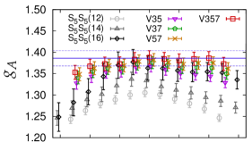
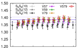
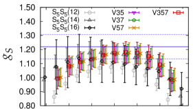
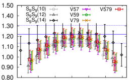
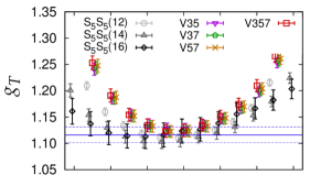
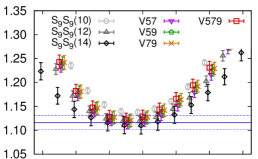
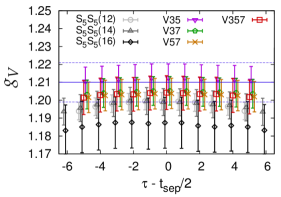
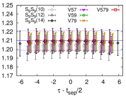
Our conclusion on the variational method, looking especially at the data for $g_{A}$, is that one needs the full $3\times 3$ variational ansatz V357 if the smearing size is restricted to $\sigma\leq 7$. In the case of V579, one finds that V79 and V579 give consistent estimates, so a $2\times 2$ analysis may be sufficient. The conservative approach, in the absence of detailed information on the smearing sizes to use, would be to use a $3\times 3$ variational ansatz if results with $<2\%$ total uncertainty are desired.

In Fig. 15, we compare the estimates for the unrenormalized isovector charges $g_{A}$, $g_{S}$, $g_{T}$ and $g_{V}$ obtained from the 2-state fit to R1 data with $\sigma=5$ and $t_{\rm sep}=[12,14,16,18]$ with the R4 data with $\sigma=9$ and $t_{\rm sep}=[10,12,14,16]$. We also show the $3\times 3$ variational estimates V357 (R2) and V579 (R3) obtained using $t_{\rm sep}=12$. Comparing the two methods we find:

• The excited-state effect in $g_{A}$ in the $S_{5}S_{5}$ data is large but the 2-state ansatz fits the data and gives a $t_{\rm sep}\to\infty$ estimate that agrees with the V357 and V579 values.

• The excited-state contamination in $g_{A}$ is much smaller in the $S_{9}S_{9}$ data. However, since the data with $t_{\rm sep}=10,12,14$ overlap, the fit gives a $t_{\rm sep}\to\infty$ estimate that is about $1\sigma$ below the V357 and V579 estimates. (It is also about $1\sigma$ below the estimate from the fit to $S_{5}S_{5}$ data as shown in Fig. 13.) The combined one sigma difference between the overlapping $t_{\rm sep}=10,12,14$ data and the $t_{\rm sep}=16$ data reduces the confidence in the 2-state fit. This case highlights a generic problem: for the 2-state fit to give the $t_{\rm sep}\to\infty$ estimate with $<1\%$ error, the statistics have to be large enough that the trend in the data is resolved at at least three values of $t_{\rm sep}$ .

• In lattice calculations with dynamical fermions, the factor limiting the statistics is the number of independent gauge configurations available. For a fixed statistical sample, the errors in our data increase by $\approx 80\%$ with each two units of $\mathop{t_{\rm sep}}\nolimits$ as discussed previously. Consequently, the error in the 2-state fit estimate increases as data at larger $\mathop{t_{\rm sep}}\nolimits$ are included in the multiple $\mathop{t_{\rm sep}}\nolimits$ analysis to get the $t_{\rm sep}\to\infty$ value. For example, the estimates for $g_{A}$, using R1 with $S_{5}S_{5}$, are 1.353(18), 1.366(20), 1.378(22), 1.382(25), 1.395(29), and 1.424(44) with fits to $\mathop{t_{\rm sep}}\nolimits=[10,12,14]$, $[10,12,14,16]$, $[10,12,14,16,18]$, $[12,14,16]$, $[12,14,16,18]$ and $[14,16,18]$ data, respectively. Our best estimate, 1.395(29), is obtained by neglecting the data at $\mathop{t_{\rm sep}}\nolimits=10$, which have the largest excited state contamination. In comparison, the V357 variational result with $\mathop{t_{\rm sep}}\nolimits=12$ is 1.386(16). We anticipate that the error in the variational method would also increase with $\mathop{t_{\rm sep}}\nolimits$.

• For $g_{S}$, the overall trend in the $S_{5}S_{5}$ data with $t_{\rm sep}=10,12,14,16$ is it converges from below and show significant excited-state contamination. The $S_{9}S_{9}$ data at each $t_{\rm sep}=10,12,14,16$ agree with V357 and V579 data. The excited-state contamination is manifest in all the data as the curvature with $\tau$. The 2-state fit to $S_{5}S_{5}$ and $S_{9}S_{9}$ gives an estimate consistent with V357 and V579.

• For $g_{T}$, the 2-state fits to $S_{5}S_{5}$ and $S_{9}S_{9}$ data with $t_{\rm sep}=[12,14,16,18]$ and $t_{\rm sep}=[10,12,14,16]$, respectively, give consistent results and are about $1\sigma$ below V357 and V579. Surprisingly, the $S_{5}S_{5}$ data show smaller curvature than $S_{9}S_{9}$ data. Overall, excited-state contamination is smaller than in $g_{A}$ and $g_{S}$ with the total variation with $\mathop{t_{\rm sep}}\nolimits$ at the central value of $\tau$ being $\raisebox{-3.01385pt}{$\stackrel{{\scriptstyle\textstyle<}}{{\sim}}$ }5\%$.

• All estimates for $g_{V}$ are consistent within $1\%$ uncertainty. The largest difference is between the $S_{5}S_{5}$ and $S_{9}S_{9}$ estimates, which is about $1\sigma$.

To summarize, our comparison shows that once good choices of the smearing sizes and $t_{\rm sep}$ are known, the two methods give reliable and consistent results but the variational estimates have smaller errors with the same statistics because they were obtained from a smaller value of $\mathop{t_{\rm sep}}\nolimits$.

Figure 15: Comparison of estimates for the unrenormalized isovector charges $g_{A}$, $g_{S}$, $g_{T}$ and $g_{V}$ from the variational analysis V357 (R2) and V579 (R3) with (left) R1 data with $\sigma=5$ and (right) R4 data with $\sigma=9$. The gray error band and the solid line within it is the $t_{\rm sep}\to\infty$ estimate from the 2-state fit using (left) $S_{5}S_{5}$ data with $t_{\rm sep}=[12,14,16,18]$ and (right) $S_{9}S_{9}$ using data with $t_{\rm sep}=[10,12,14,16]$.

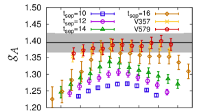
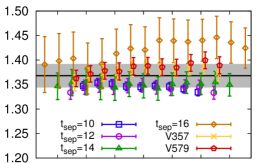
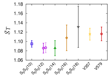
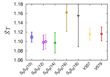
The important question is the following: does the consistency of the four analyses confirm that the $\mathop{t_{\rm sep}}\nolimits\to\infty$ value has been obtained? In Fig. 16, we compare the trends in the estimates of $g_{A}$ and their errors by making independent 2-state fits with $\langle 1|\mathcal{O}_{\Gamma}|1\rangle=0$ to data at a fixed value of $t_{\rm sep}$. We find that the estimates from the $S_{5}S_{5}$ data increase with $\mathop{t_{\rm sep}}\nolimits$. This behavior is consistent with the general trend observed in all the data—the estimate of $g_{A}$ converge from below. Even though the total variation between $\mathop{t_{\rm sep}}\nolimits=10$ and $18$ estimates is less than 3$\sigma$, taken at face value, this trend would indicate that the V357 and V579 results are underestimates. On the other hand, the incremental increase with $\mathop{t_{\rm sep}}\nolimits$ has to go to zero at sufficiently large $\mathop{t_{\rm sep}}\nolimits$. Unfortunately, the errors in the $\mathop{t_{\rm sep}}\nolimits\geq 16$ estimates, crucial to determining the value of $\mathop{t_{\rm sep}}\nolimits$ by which the asymptotic value is reached, are too large.

Figure 16: Comparison of estimates of the unrenormalized $g_{A}$ from the $S_{5}S_{5}$ data (left) and the $S_{9}S_{9}$ data (right) for different values of $\mathop{t_{\rm sep}}\nolimits$ with V357 and V579. In each case, the fit is made to data from a single $t_{\rm sep}$, given within parentheses, using the 2-state ansatz with $\langle 1|\mathcal{O}_{\Gamma}|1\rangle=0$. We show the data and the fits (bottom panels) and a comparison of the resulting estimating of $g_{A}$ (top panels). For clarity, the $\mathop{t_{\rm sep}}\nolimits=18$ data shown in Fig. 13, are not reproduced here. The data points in black on either end in the variable $\tau$ are not used in the fits. The second estimates for $S_{5}S_{5}(12)$ and $S_{9}S_{9}(12)$ from R3 are shown with dotted error bars. The $1\sigma$ difference between the two $S_{9}S_{9}(12)$ estimates is discussed in the text and the data shown in Fig. 2.

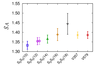
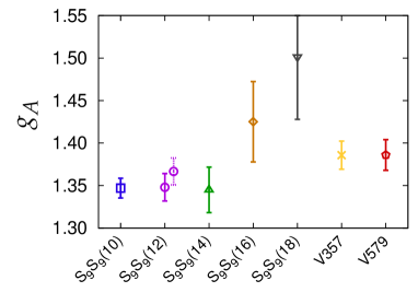
The situation is not resolved by the $S_{9}S_{9}$ data as they do not show a uniform trend—the data with $\mathop{t_{\rm sep}}\nolimits=10,\ 12$ and $14$ are flat and below V357 and V579, whereas the $\mathop{t_{\rm sep}}\nolimits=16$ and $18$ data are above but their significance is less as they have large errors. Since the differences are about one combined sigma, it is hard to quantify trends with current statistics. For example, as shown in the top right panel of Fig. 16, the two $S_{9}S_{9}(12)$ data points from R3 and R4 (see Fig. 2 for the data versus $\tau$) differ by $1\sigma$. If we use the $S_{9}S_{9}(12)$ point from R3 (shown with the dotted error bar) to determine the trend, we would conclude that the $S_{9}S_{9}$ data also show a rising trend and the observed consistency of $\mathop{t_{\rm sep}}\nolimits=10,\ 12$ and $14$ estimates from R4 is a statistical fluctuation. No such fluctuation is seen in the two $S_{5}S_{5}(12)$ data points from R1 and R3 plotted in the top left panel of Fig. 16.

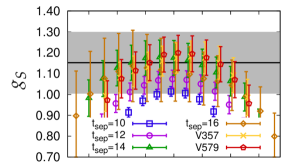
A comparison of the estimates in Fig. 17, where we plot all the results obtained from data with $\mathop{t_{\rm sep}}\nolimits=12$, shows that the errors in the V357 (V579) result are comparable to those in $S_{5}S_{5}(12)$ ($S_{9}S_{9}(12)$) with the same statistics but with less excited-state contamination. Equally important, the trends in the data in Figs. 16 and 17 show that the error estimates in the $t_{\rm sep}\to\infty$ values for $S_{5}S_{5}$ and $S_{9}S_{9}$, given in Table 5, are reasonable and cover the uncertainties discussed here.

Figure 17: Comparison of the estimates of the unrenormalized charges obtained using a 2-state fit with $\langle 1|\mathcal{O}_{\Gamma}|1\rangle=0$ to all the $\mathop{t_{\rm sep}}\nolimits=12$ data. The data point with solid error bars are from R2, dotted from R3 and dashed from R4.

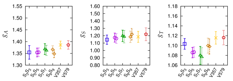
We compare the behavior of $g_{T}$ in Figs. 17 and 18. The overall trend, that $g_{T}$ converges from above, would imply that the $\mathop{t_{\rm sep}}\nolimits=10,\ 12$ and $14$ estimates from both the $S_{5}S_{5}$ and $S_{9}S_{9}$ data are better estimates of the $t_{\rm sep}\to\infty$ value and lie about $1\sigma$ below V357 and V579 results. On the other hand, with current statistics, all the estimates are consistent within one combined $\sigma$. Note that, unlike $g_{A}$, the two sets of results for $S_{9}S_{9}(12)$ and also those for $S_{5}S_{5}(12)$ and $S_{7}S_{7}(12)$, obtained using different source positions, are in very good agreement.

Figure 18: Comparison of estimates of the unrenormalized $g_{T}$ from the $S_{5}S_{5}$ data (left) and the $S_{9}S_{9}$ data (right) for different values of $\mathop{t_{\rm sep}}\nolimits$ with V357 and V579. The rest is the same as in Fig. 16.

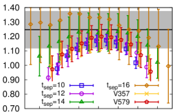
The comparison of the scalar charge $g_{S}$ is shown in Figs. 17 and 19. The data are consistent within their much larger error estimates and no trend with $\mathop{t_{\rm sep}}\nolimits$ is apparent. Also, similar to the case of $g_{T}$, the two independent estimates of $g_{S}$ from $S_{5}S_{5}(12)$, $S_{7}S_{7}(12)$ and $S_{9}S_{9}(12)$ are in very good agreement.

Figure 19: Comparison of estimates of the unrenormalized $g_{S}$ from the $S_{5}S_{5}$ data (left) and the $S_{9}S_{9}$ data (right) for different values of $\mathop{t_{\rm sep}}\nolimits$ with V357 and V579. The rest is the same as in Fig. 16.

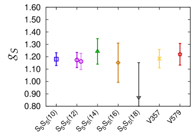
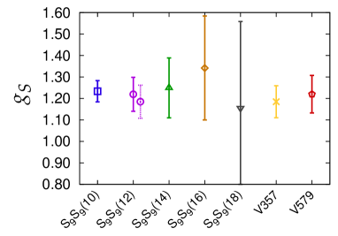
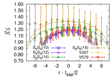
Our overall conclusion, based on the data shown in Figs. 16, 17, 18 and 19 that compare results from fixed $\mathop{t_{\rm sep}}\nolimits$ analyses, is that the errors in the V357 (V579) estimates are similar to those in the $S_{5}S_{5}$ ($S_{9}S_{9}$) values with the same $t_{\rm sep}=12$, but the excited-state contamination in $g_{A}$ is smaller. In the case of $g_{S}$, the errors are large and all the estimates are consistent. There is a small but consistent trend indicating an increase in the estimates of $g_{A}$ and $g_{S}$ towards the $t_{\rm sep}\to\infty$ value with $\mathop{t_{\rm sep}}\nolimits$. The situation with $g_{T}$ is less clear. Considering the results for all the three charges, we again conclude that a smearing size $\sigma\approx 7$ is optimal for a 2-state fit analysis with multiple $\mathop{t_{\rm sep}}\nolimits$. In the variational analysis, there is no significant difference between V357 and V579.

Lastly, we briefly comment on the similar behavior of excited-state contamination observed in the calculation of nucleon matrix elements and its dependence on smearing parameters and $\mathop{t_{\rm sep}}\nolimits$ by other lattice QCD collaborations Bali et al. (2015); Abdel-Rehim et al. (2015); Capitani et al. (2015); Djukanovic et al. (2015). These three collaborations first use different amounts of APE smearing to smooth the links and then construct smeared sources using Wuppertal (Gaussian) smearing. A detailed comparison of their results with our analysis is not straightforward because each collaboration has used different smearing methods, smearing sizes and values of $\mathop{t_{\rm sep}}\nolimits$ on different ensembles. For example, translating RQCD collaboration’s  Bali et al. (2015) parameters would give smearing sizes between 0.7–0.9 fm on their various ensembles. The smearing size used by the ETMC collaboration is $\approx 0.5$ fm and they report similar excited-state contamination in the extraction of all the charges Abdel-Rehim et al. (2015). The Mainz group Capitani et al. (2015); Djukanovic et al. (2015) also tunes the smearing size to $\approx 0.5$ fm in their study of electric and magnetic form factors. Our work shows that the size of the excited-state contamination in the extraction of various charges and form factors is sensitive to the smearing parameters and values of $\mathop{t_{\rm sep}}\nolimits$ simulated. It is, therefore, important to demonstrate that the $\mathop{t_{\rm sep}}\nolimits\to\infty$ value has been obtained and compare errors in this limit.

V Which Method is More Cost Effective?

In the previous Sec. IV, we showed that both the 2-state fit with data at multiple $t_{\rm sep}$ and the variational analysis with multiple smearings can be made essentially equally effective in reducing excited-state contamination and give overlapping estimates. The errors in the variational analysis are, however, 35–60% smaller compared to the estimates from the $S_{9}S_{9}$ 2-state analysis with multiple $\mathop{t_{\rm sep}}\nolimits$ as shown in Table 5. Comparing data at fixed $\mathop{t_{\rm sep}}\nolimits=12$ shows that the variational method yields estimates closer to the asymptotic value for $g_{A}$, while for $g_{S}$ the two estimates $S_{7}S_{7}(12)$ and $S_{9}S_{9}(12)$ are as good. The trend in $g_{T}$ is not clear, but if the convergence from above is validated by higher precision data, then $S_{7}S_{7}(12)$ would be the preferred estimate. Being able to obtain the $t_{\rm sep}\to\infty$ estimate from the smallest value of $\mathop{t_{\rm sep}}\nolimits$ is important because the errors grow by $\approx 80\%$ for every two units of $t_{\rm sep}$.

To decide between the two methods—variational versus the 2-state fit to data at multiple $t_{\rm sep}$, we present a cost-benefit analysis assuming that the best value of the smearing parameter $\sigma$ (for example, $\sigma=7$ in this work) has already been determined using trial runs. Also, based on the discussion in Sec. IV, we will mostly use $g_{A}$, and its extrapolation to $t_{\rm sep}\to\infty$, to compare the two methods as it shows large excited-state contamination. Next, based on the $S_{5}S_{5}$ and $S_{9}S_{9}$ data, we assume that the errors in a 2-state fit to $S_{7}S_{7}$ data with $\mathop{t_{\rm sep}}\nolimits=10,\ 12,\ 14$ and $16$ will be about $50\%$ larger than those from V579. Lastly, we assume that the sequential $u$ and $d$ propagators are calculated using the coherent sequential source trick with $N_{\rm meas}$ source locations being processed simultaneously on each configuration. Keeping in mind that the goal is to get the best estimate for the $t_{\rm sep}\to\infty$ value with a fixed computational cost, we count the number of inversions of the Dirac matrix required for the minimum computation in each case as follows.

• A 2-state fit with $N_{\rm tsep}$ values of $t_{\rm sep}$ requires $N_{\rm meas}+2\times N_{\rm tsep}$ inversions: Our analyses indicate that $N_{\rm tsep}=3$ is sufficient and $N_{\rm tsep}=4$ allows for validation. Typical values of $N_{\rm meas}$ on lattice sizes currently being used are either 3 or 4. For $N_{\rm meas}=3$, one needs 9 inversions for $N_{\rm tsep}=3$ and 11 for $N_{\rm tsep}=4$. Doubling the statistics to improve the fit would increase the cost to 22 inversions for $N_{\rm tsep}=4$. However, recognizing that the reduction in errors is required mainly in our $\mathop{t_{\rm sep}}\nolimits=16$ data, doubling its statistics would increase the cost to 16 inversions.

• A variational analysis with $N_{\rm smear}$ smearings requires $N_{\rm smear}\times N_{\rm meas}+(2\times N_{\rm smear}\times N_{\rm smear})\times N_{\rm tsep}$ inversions if all combinations of the source and sink 3-point functions are calculated. Our analysis suggests that $N_{\rm smear}=3$ is needed for high precision. In that case, for $N_{\rm meas}=3$ and $N_{\rm tsep}=1$ one needs 27 inversions.

  This cost can be reduced significantly if a good estimate of the eigenvector $u_{0}$ used for constructing the projected variational correlation function is known before starting the calculation of the 3-point functions. In that case the dot product of the $N_{\rm smear}\times N_{\rm smear}$ matrix of zero-momentum nucleon sources at the sink with $u_{0}$ can be taken before the final inversion to construct the sequential propagators. This trick would reduce the number of sequential propagators to calculate from $2\times N_{\rm smear}\times N_{\rm smear}$ to $2\times N_{\rm smear}$. For each of the $N_{\rm smear}$ projected sources, the coherent source can be constructed in the same way as before, i.e., by repeating the operation on the $N_{\rm meas}$ time slices and adding the sources after projection using $u_{0}$. With this simplification, the cost is reduced to $N_{\rm smear}\times N_{\rm meas}+(2\times N_{\rm smear}\times N_{\rm tsep})$ inversions, which for $N_{\rm meas}=N_{\rm smear}=3$ and $N_{\rm tsep}=1$ is 15 inversions and increases to 21 for $N_{\rm tsep}=2$. Lastly, we anticipate, based on the $S_{5}S_{5}$ and $S_{9}S_{9}$ analyses showing that the errors increase by a factor of $\approx 0.8$ for increase in $\mathop{t_{\rm sep}}\nolimits$ by two units, that a similar increase would be present in the variational analysis, i.e., errors in a $\mathop{t_{\rm sep}}\nolimits=14$ variational calculation, done to confirm that the $\mathop{t_{\rm sep}}\nolimits\to\infty$ value has been obtained, would be larger by a factor of $\approx 1.8$.

In Sec. IV, we found that estimates of $g_{S}$, $g_{T}$, and $g_{V}$ from a 2-state fit to just the $t_{\rm sep}=16$ data are also compatible with those from the variational analysis but the errors are larger by a factor of about two. To raise the precision of the 2-state fit with $N_{\rm tsep}=4$ to the level of the variational result, i.e., achieve comparable errors, we would need to roughly double the statistics. In this scenario, the computational cost of a $3\times 3$ variational analysis with a good estimate of $u_{0}$ would be more cost effective (15 versus $2\times 11=22$ inversions). However, if the statistics for only the $\mathop{t_{\rm sep}}\nolimits=16$ data is doubled, then the 2-state fit is equally cost effective (15 versus 16 inversions).

In the most conservative approach, assuming two values of $t_{\rm sep}$ need to be simulated in the variational approach to demonstrate convergence to the $t_{\rm sep}\to\infty$ estimate, as indicated by the discussion in Sec. IV, or one needs double the statistics in the 2-state state fit with $N_{\rm tsep}=4$, the two methods are again equally cost effective (21 versus 22 inversions).

The cost effectiveness of the 2-state fit method increases as the quark mass is reduced and the lattice size $T$ is increased. On our $64^{3}\times 128$ lattices at $M_{\pi}\approx 200$ MeV we can use $N_{\rm meas}=5$ or even $6$ since the signal in the nucleon 2-point correlation function dies out by $t\approx 20$. For $N_{\rm meas}=5$, the 2-state fit with $N_{\rm tsep}=4$ would cost 13 inversions, while a $N_{\rm smear}=3$ variational analysis with $t_{\rm sep}=1$ and known $u_{0}$ would cost 21 inversions.

A somewhat different conclusion is reached in Ref. Dragos et al. (2015), in which the authors claim that the variational method offers a more efficient and robust method for the determination of the nucleon matrix elements. Some of the reasons for their conclusion that the variational method is decidedly better are:

• Their calculation was done on a finer lattice with $a=0.074$ fm. Thus, to first approximation, all our length scales should be multiplied by $1.1$ when comparing with their analysis.

• The much higher statistical precision of our calculation (42,528 versus 1050 measurements) allows us to better resolve the trends in both methods.

• Their variational analysis was done with three smearing sizes, $\sigma\approx 4.1,5.8$ and $8.3$. These three sizes cover the value $\sigma=7.7$ corresponding to $\sigma\approx 0.57$ fm we consider optimal. Thus, we expect their analysis to give a good estimate with $t_{\rm sep}=13$, which, in physical units, is equivalent to the $t_{\rm sep}=12$ used in our variational analysis.

• Their 2-state fits were based on data with $\sigma\approx 4.1$ ($N_{\rm GS}=32$), for which the excited-state contamination is very large as shown in this work. With such an unoptimized value of $\sigma$ and given that their data for $g_{A}$ with $t_{\rm sep}=16,19$ and $22$ has large errors, it is not surprising that their $t_{\rm sep}\to\infty$ estimate from a 2-state fit has much larger errors compared to their variational estimate. For the same reasons, we suspect that their 2-state fit slightly underestimates the $t_{\rm sep}\to\infty$ value.

• They do not provide a cost estimate for the two analyses. Assuming that they constructed the full $3\times 3$ matrix of 3-point correlation functions in their variational analysis, it is 13 versus 27 inversions for the 2-state versus the variational approach.

• They did not evaluate the change in the cost effectiveness of the two methods as the quark mass is decreased and the lattice size $T$ is increased correspondingly. With larger $N_{\rm meas}$, the relative cost effectiveness of the 2-state fit method increases.

To summarize, we have compared the two methods using the optimal smearing sizes. Our conclusion on cost effectiveness is based on the best case scenario of a tuned value of $\sigma$ for both methods and using three smearing sizes with a known result for $u_{0}$ in the variational analysis. We have also assumed that the same choice of the smearing parameters and $t_{\rm sep}$ are equally effective for all matrix elements. We find that both methods give results that are consistent within errors. The variational method is more cost effective if results at a single value of $t_{\rm sep}$ are sufficient to obtain the $t_{\rm sep}\to\infty$ value and a good estimate of $u_{0}$ is known beforehand. The 2-state fit with four values of $t_{\rm sep}$ and double the statistics at the larger $\mathop{t_{\rm sep}}\nolimits$ values has the advantage of the built in check of the convergence to the $t_{\rm sep}\to\infty$ estimate that can be made separately for each observable. Lastly, the cost effectiveness of the 2-state fit method increases as the lattice size $T$ is increased and the quark mass is lowered to its physical value because a larger number of measurements, $N_{\rm meas}$, can be made simultaneously on each configuration and $N_{\rm meas}$ sources at the sink timeslice added in the coherent source method to produce the sequential propagator.

VI Conclusions

We have presented a high statistics study of isovector charges of the nucleon using (2+1)-flavor clover lattices generated using the RHMC algorithm. The focus of this work is to investigate methods to improve the statistical precision of the data and reduce the excited-state contamination in matrix elements of quark bilinear operators within nucleon states. We show that both the variational method and the 2-state fit with data at multiple $\mathop{t_{\rm sep}}\nolimits$ are equally effective at reducing excited-state contamination once the smearing parameters and the values of $\mathop{t_{\rm sep}}\nolimits$ have been tuned.

With the current lattice parameters, our ability to conclude which method gives a more reliable estimate of the $t_{\rm sep}\to\infty$ value and is more cost effective is limited by statistics since all the estimates are consistent within $1\sigma$ error estimates. To demonstrate that the $t_{\rm sep}\to\infty$ estimate has been obtained requires doing the variational calculation at two values of $\mathop{t_{\rm sep}}\nolimits$ and in the 2-state fit using at least 3 values of $\mathop{t_{\rm sep}}\nolimits$ with $\mathop{t_{\rm sep}}\nolimits\geq 1$ fm in both cases. The advantage of simulating multiple values of $\mathop{t_{\rm sep}}\nolimits$ in either method is to be able to evaluate the convergence to the $t_{\rm sep}\to\infty$ limit as a function of $\mathop{t_{\rm sep}}\nolimits$. The cost of adding additional values of $\mathop{t_{\rm sep}}\nolimits$ is much less in the 2-state fit method compared to a $3\times 3$ variational analysis.

For a fixed number of gauge configurations available and measurements made, the errors in the variational method with a fixed $\mathop{t_{\rm sep}}\nolimits$($\approx 1$ fm in our study) are consistent with those from the 2-state fit to data with the same $\mathop{t_{\rm sep}}\nolimits$ but the excited-state contamination is smaller, so it gives a better estimate of the $t_{\rm sep}\to\infty$ limit. The error in the 2-state fit with multiple $\mathop{t_{\rm sep}}\nolimits$ method are larger because data with/at larger $\mathop{t_{\rm sep}}\nolimits$ are needed to reduce excited-state contamination and errors in the data for the 3-point functions grow rapidly with $\mathop{t_{\rm sep}}\nolimits$.

Assuming that the $t_{\rm sep}\to\infty$ estimate has been obtained in all four runs R1–R4 analyzed in this study with $a=0.081$ fm, $M_{\pi}=312$ MeV lattices of size $T=64$ and $N_{\rm meas}=3$, the $3\times 3$ variational method is computationally more cost effective than the 2-state fit to data at four values of $\mathop{t_{\rm sep}}\nolimits$ because the errors are about $50\%$ smaller. The cost becomes the same if one doubles the statistics in the 2-state method to make the errors roughly equal and simulates a second $\mathop{t_{\rm sep}}\nolimits$ in the variational calculation to confirm the convergence to the $t_{\rm sep}\to\infty$ limit.

The cost effectiveness of the 2-state method increases rapidly as the light quark mass is reduced towards its physical value and the lattice size $T$ is increased correspondingly because the number of simultaneous measurements, $N_{\rm meas}$, that can be made on each configuration and benefit from the coherent sequential source method increases with $T$. Since the cost of the lattice calculations at a fixed value of the lattice spacing is dominated by the analysis of ensembles close to the physical values of the quark mass, one should carefully choose the method that is more cost effective in that limit.

Our overall conclusion is that both methods are effective in reducing the excited-state contamination and have their relative strengths. The choice depends on the number of gauge configurations available, the value of the light quark mass, the lattice size, and the effort needed to tune the smearing parameters, the eigenvector $u_{0}$ and the values of $\mathop{t_{\rm sep}}\nolimits$ adequately prior to the calculation of the 3-point functions.