2016 \jvol54 \fstpage529 \endpage596 10.1146/annurev-astro-081915-023441
The Galaxy in Context: Structural, Kinematic & Integrated Properties
Abstract
Our Galaxy, the Milky Way, is a benchmark for understanding disk galaxies. It is the only galaxy whose formation history can be studied using the full distribution of stars from faint dwarfs to supergiants. The oldest components provide us with unique insight into how galaxies form and evolve over billions of years. The Galaxy is a luminous () barred spiral with a central box/peanut bulge, a dominant disk, and a diffuse stellar halo. Based on global properties, it falls in the sparsely populated “green valley” region of the galaxy colour-magnitude diagram. Here we review the key integrated, structural and kinematic parameters of the Galaxy, and point to uncertainties as well as directions for future progress. Galactic studies will continue to play a fundamental role far into the future because there are measurements that can only be made in the near field and much of contemporary astrophysics depends on such observations.
keywords:
Galaxy: Structural Components, Stellar Kinematics, Stellar Populations, Dynamics, Evolution; Local Group; Cosmology1 PROLOGUE
Galactic studies are a fundamental cornerstone of contemporary astrophysics. Nowadays, we speak of near-field cosmology where detailed studies of the Galaxy underlie our understanding of universal processes over cosmic time (Freeman & Bland-Hawthorn, 2002). Within the context of the cold dark matter paradigm, the Galaxy built up over billions of years through a process of hierarchical accretion (see Fig. 1). Our Galaxy has recognisable components that are likely to have emerged at different stages of the formation process. In particular, the early part of the bulge may have collapsed first seeding the early stages of a massive black hole, followed by a distinct phase that gave rise to the thick disk. The inner halo may have formed about the same time while the outer halo has built up later through the progressive accretion of shells of material over cosmic time (Prada et al., 2006). The dominant thin disk reflects a different form of accretion over the same long time frame (Brook et al., 2012).
We live in an age when vast surveys have been carried out across the entire sky in many wavebands. At optical and infrared wavelengths, billions of stars have been catalogued with accurate photometric magnitudes and colours (Skrutskie et al., 2006; Saito et al., 2012; Ivezić, Beers & Jurić, 2012). But only a fraction of these stars have high quality spectral classifications, radial velocities and distances, with an even smaller fraction having useful elemental abundance determinations. The difficulty of measuring a star’s age continues to hamper progress in Galactic studies, but this stumbling block will be partly offset by the ESA gaia astrometric survey already under way. By the end of the decade, this mission will have measured accurate distances and velocity vectors for many millions of stars arising from all major components of the Galaxy (de Bruijne et al., 2015). In light of this impending data set, we review our present understanding of the main dynamical and structural parameters that describe our home, the Milky Way.
| Distance of Sun from the Galactic Centre (§3.2) | |
| Distance of Sun from the Galactic Plane (§3.3) | |
| Circular speed, angular velocity at Sun with respect to Galactic Centre (§3.4, §6.4.2) | |
| , , component of solar motion with respect to LSR (§5.3.3) | |
| Solar motion with respect to LSR (§5.3.3) | |
| Possible LSR streaming motion with respect to (§5.3.3, §6.4.2) | |
| , | Oort’s constants (§6.4.2) |
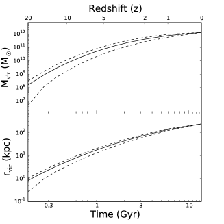
| Galactic virial radius (§6.3) | |
| , | Galactic virial mass, virial timing mass (§6.3) |
| , | Galactic stellar mass, global star formation rate (§2.2, §6.4) |
| , b | Galactic baryon mass, baryon fraction (§6.2, §6.4.3) |
| , , | Bulge dynamical mass and stellar mass, classical bulge fraction (§4.2.4) |
| Half-mass bulge velocity dispersions in and rms (§4.2.3) | |
| , | b/p-bulge orientation and axis ratio from top (§4.2.1) |
| , | Central vertical scale-height and edge-on axis ratio of b/p-bulge (§4.2.1) |
| Radius of maximum X (§4.2.1) | |
| , | Stellar masses of thin and superthin long bar (§4.3) |
| , | Long bar orientation and half-length (§4.3) |
| , | Vertical scale heights of thin and superthin long bar (§4.3) |
| , | Bar pattern speed and corotation radius (§4.4) |
| , | Mass and dynamical influence radius of supermassive black hole (§3.4) |
| , | Masses of nuclear star cluster and nuclear stellar disk (§4.1) |
| , | Nuclear star cluster half-mass radius and axis ratio (§4.1) |
| , | Nuclear stellar disk break radius and vertical scale-height (§4.1) |
| Coronal (hot) halo mass (§6.2) | |
| , | Stellar halo mass and substructure mass (§6.1.2) |
| , , | Stellar halo inner, outer density slope, break radius (§6.1.1) |
| , | Inner and outer mean flattening (§6.1.1) |
| Stellar halo velocity dispersions in , , near the Sun (§6.1.3) | |
| Local halo rotation velocity (§6.1.3) | |
| , | Thin, thick disk stellar masses (§5.1.3, §5.2.2) |
| , | Thin, thick disk exponential scalelength in (§5.1.3, §5.2.2) |
| , | Thin, thick disk exponential scaleheight in (§5.1.3) |
| , | Thick disk fraction in local density, in integrated column density (§5.1.3) |
| , | Old thin disk velocity dispersion in , at 10 Gyr (§5.4) |
| , | Thick disk velocity dispersion in , (§5.4) |
| , , | Local mass surface density, mass density, dark matter energy density (§5.4.2) |
aOur convention is to use for a projected radius in two dimensions (e.g. disk) and for a radius in three dimensions (e.g. halo). b is the ratio of baryonic mass to total mass integrated to a radius where both quantities have been determined (e.g. ).
We run into a problem familiar to cartographers. How is one to describe the complexity of the Galaxy? No two galaxies are identical; even the best morphological analogues with the Milky Way have important differences (Fig. 2). Historically, astronomers have resorted to defining discrete components with the aim of measuring their structural parameters (see Table 1). We continue to see value in this approach and proceed to define what we mean by each subsystem, and the best estimates that can be made at the present time. In reality, these ‘components’ exhibit strong overlap by virtue of sharing the same evolving Galactic potential (e.g. Guedes et al., 2013) and the likelihood that stars migrate far from their formation sites (Sellwood & Binney, 2002; Minchev & Famaey, 2010).
Even with complete data (density field, distribution function, chemistry), it is unlikely that any one component can be entirely separated from another. In particular, how are we to separate the bar/bulge from the inner disk and inner halo? A distinct possibility is that most of our small bulge (compared to M31) has formed through a disk instability associated with bar formation, rather than during a dissipational early collapse phase. The same challenge exists in separating the thin disk from the thick disk. Some have argued for a gradual transition but there is now good evidence that a major part of the thick disk is chemically distinct from the dominant thin disk, suggesting a different origin. In this context, Binney (2013) has argued that the Galaxy’s stellar populations are better described by phase-space distribution functions (DF) that are self-consistent with the underlying gravitational potential (§5).
Our goal here is to identify the useful structural and kinematic parameters that aid comparison with other galaxies and place our Galaxy in context. These “measurables” are also important for comparing with numerical simulations of synthetic galaxies. A simulator runs a disk simulation and looks to compare the evolutionary phase where the bar/bulge instability manifests itself. In principle, only a statistical ‘goodness of fit’ is needed without resorting to any parametrisation (Sharma et al., 2011). But in practice, the comparison is likely to involve global properties like rotation curves, scale lengths, total mass (gas, stars, dark matter), stellar abundances and the star formation history. Here we focus on establishing what are the best estimates for the Galaxy’s global properties and the parameters that describe its traditional components.
Kerr & Lynden-Bell (1986) revisited the 1964 IAU standards for the Sun’s distance and circular velocity ( kpc; km s-1) relative to the Galactic Centre and proposed a downward revision ( kpc; km s-1). Both values can now be revised further to reflect the new observational methods at our disposal three decades on. Our goal in this review is to provide an at-a-glance summary of the key structural and kinematic parameters to aid the increasing focus on Galactic studies. For reasons that become clear in later sections, we cannot yet provide summary values that are all internally consistent in a plausible dynamical description of the Galaxy; this is an important aim for the next few years. For more scientific context, we recommend reviews over the past decade that consider major components of the Galaxy: Helmi (2008), Ivezić, Beers & Jurić (2012), Rix & Bovy (2013) and Rich (2013).
This is an era of extraordinary interest and investment in Galactic studies exemplified above all by the gaia astrometric mission and many other space-based and ground-based surveys. In the next section (§2), we provide a context for these studies. The Galaxy is then described in terms of traditional components: Galactic Centre (§3), Inner Galaxy (§4), Disk Components (§5) and Halo (§6). Finally, we discuss the likely developments in the near term and attempt to provide some pointers to the future (§7).
2 THE GALAXY IN CONTEXT
We glimpse the Galaxy at a moment in time when globally averaged star formation rates (SFR) are in decline and nuclear activity is low. In key respects, the Milky Way is typical of large galaxies today in low density environments (Kormendy et al., 2010), especially with a view to global parameters (e.g. current SFR , baryon fraction ) given its total stellar mass (cf. de Rossi et al., 2009), as we discuss below. But in other respects, it is relatively unusual, caught in transition between the ‘red sequence’ of galaxies and the ‘blue cloud’ (Mutch, Croton & Poole, 2011). Moreover, unlike M31, our Galaxy has not experienced a major merger for the past 10 Gyr indicating a remarkably quiescent accretion history for a luminous galaxy (Stewart et al., 2008). Most galaxies lie near the turnover of the galaxy luminosity function where star formation quenching starts to become effective (Benson et al., 2003). But this may not be the last word for the Galaxy: the Magellanic gas stream is evidence for very substantial ( ) and ongoing gas accretion in the present day (Putman et al., 1998; Fox et al., 2014). The Galaxy stands out in another respect: it is uncommon for an galaxy to be orbited by two luminous dwarf galaxies that are both forming stars (Robotham et al., 2012). None the less, the Galaxy will always be the most important benchmark for galaxy evolution because it provides information that few other galaxies can offer the fully resolved constituents that make up an galaxy in the present epoch.
2.1 Environment & Evolution
The Galaxy is one of the two dominant members of the Local Group, a low-mass system constituting a loosely bound collection of spirals and dwarf galaxies. The Local Group has an internal velocity dispersion of about 60 km s-1 (van den Bergh, 1999) and is located in a low-density filament in the far outer reaches of the Virgo supercluster of galaxies (Tully et al., 2014). Galaxy groups with one or two dominant spirals are relatively common, but close analogues of the Local Group are rare. The presence of an infalling binary pair the Small and Large Magellanic Clouds (SMC, LMC) around an galaxy is only seen in a few percent of cases in the Galaxy and Mass Assembly (gama) survey (Driver et al., 2011). This frequency drops to less than 1% if we add the qualification that the massive binary pair are actively forming stars.
With a view to past and future evolution, it is instructive to look at numerical simulations of the Local Group. The Constrained Local Universe Simulations the clues project (www.clues-project.org) are optimised for a study of the formation of the Local Group within a cosmological context (Forero-Romero et al., 2013; Yepes, Gottlöber & Hoffman, 2014). The accretion history of the Local Group is relatively quiet, consistent with its cold internal dynamics. The largest simulations with the most advanced prescriptions for feedback (e.g. fire, Hopkins et al., 2014) are providing new insight on why only a small fraction of the dark minihalos in orbit about the Galaxy are visible as dwarf galaxies (Wetzel et al., 2016). But we are still a long way from a detailed understanding of how the dark matter and baryons work together to produce present day galaxies.
The future orbital evolution and merging of the Local Group has been considered by several groups (Cox & Loeb, 2008; van der Marel et al., 2012a; Peebles & Tully, 2013). These models are being successively refined as proper motions of stars in M31 become available. We learn that the Galaxy and M31 will reach pericentre passage in about 4 Gyr and finally merge in 6 Gyr. The models serve to remind us that the Galaxy is undergoing at least three strong interactions (LMC, SMC, Sgr) and therefore cannot be in strict dynamical equilibrium. This evolution can be accommodated in terms of structural and kinematic parameters (adiabatic invariants) that are slowly evolving at present (Binney, 2013).
| Absolute magnitudea, | |||||
|---|---|---|---|---|---|
| -19.87 | -21.00 | -21.64 | -21.87 | -22.15 | |
| -20.67 | -20.70 | -21.37 | -21.90 | -22.47 | |
| Colour indexb, () | ur | ug | gr | ri | iz |
| 1.96 | 1.29 | 0.65 | 0.28 | 0.28 | |
| UV | UB | BV | VR | RI | |
| 0.86 | 0.14 | 0.73 | 0.54 | 0.58 | |
| Mass-to-light ratio, | |||||
| 1.61 | 1.77 | 1.50 | 1.34 | 1.05 | |
| 1.66 | 1.73 | 1.70 | 1.45 | 1.18 |
Magnitudes and colours derived for the Galaxy from Milky Way analogues drawn from the sdss survey using the Kroupa initial mass function. All values assume kpc and kpc for the Galaxy. aThe sdss and Johnson photometry are calibrated (typical errors 0.1 mag) with respect to the AB and Vega magnitude systems, respectively; bDifferent calibration schemes are needed for the sdss total magnitudes and the unbiassed galaxy colours which leads to inconsistencies between magnitude differences and colour indices (courtesy of Licquia, Newman & Brinchmann, 2015).
2.2 Galaxy classification & integrated properties
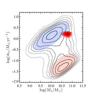
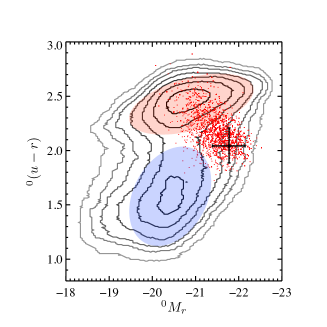
For most of the last century, galaxy studies made use of morphological classification to separate them into different classes. But high-quality, multi-band photometric and spectroscopic surveys have provided us with a different perspective (Blanton & Moustakas, 2009). The bulge to disk ratio, e.g. from Sersic index fitting to photometric images, continues to play an important role in contemporary studies (Driver et al., 2011). Many observed properties correlate with the total stellar mass and the global star formation rate . Galaxies fall into a ‘red sequence’ where star formation has been largely quenched, and a ‘blue cloud’ (‘main sequence’) where objects are actively forming stars, with an intervening ‘green valley.’ Mutch, Croton & Poole (2011) first established that the Galaxy today appears to fall in the green valley, much like M31 interestingly. Their method is based on the Copernican principle that the Galaxy is unlikely to be extraordinary given global estimates for and . In large galaxy samples, these quantities are expected to correlate closely with photometric properties like absolute magnitude and color index with a scatter of about 0.2 dex. In Fig. 3, we show the results of the most recent analysis of this kind (Licquia, Newman & Brinchmann, 2015).
Flynn et al. (2006) recapitulate the long history in deriving Galaxy global properties. Chomiuk & Povich (2011) present an exhaustive study across many wavebands and techniques to arrive at a global star formation rate for the Galaxy. They attempt to unify the choice of initial mass function and stellar population synthesis model across methods, and find 1.9 yr-1, within range of the widely quoted value of yr-1 by McKee & Williams (1997). Licquia & Newman (2015) revisit this work and conclude that yr-1 for an adopted Kroupa IMF. Likewise, there are many estimates of the Galaxy’s total stellar mass, most from direct integration of starlight and an estimate of the mass-to-light ratio, (see below), from which they estimate (§6) for a Galactocentric distance of 8.3 kpc. In §6.4, we estimate a total stellar mass of (and a revised ) from combining estimates of the mass of the bulge and the disk from dynamical model fitting to stellar surveys and to the Galactic rotation curve.
To transform these quantities into the magnitude system, one method is to select a large set of disk galaxies from the sdss photometric survey with measured bolometric properties over a spread in inclination and internal extinction. Licquia, Newman & Brinchmann (2015) select possible analogues that match and in the Galaxy given the uncertainties. In Fig. 3, we present the total absolute magnitudes and unbiassed galaxy colors for the analogues using the sdss bands; most appear to fall in the green valley, in agreement with Mutch, Croton & Poole (2011). Given these data, the likely values for the Galaxy are presented in Table 2 without the uncertainties. Note the lack of consistency between the quoted sdss magnitudes and colors because they are derived using different calibration methods as recommended for sdss DR8 (Aihara et al., 2011), but the differences are mostly below the statistical errors quoted by Licquia, Newman & Brinchmann (2015). In Fig. 3, the analogues show a lot of scatter when transformed to color-magnitude space where the green valley is less well defined. While the Galaxy’s location has moved, it still resides in the green valley.
The same inconsistency is seen in the Johnson magnitudes (Table 2) which are derived via color transformations from the sdss magnitudes (Blanton & Roweis, 2007). The cmodel and model magnitudes in bands are converted to an equivalent set of magnitudes and color indices respectively (see http://www.sdss.org/dr12/algorithms/magnitudes/#mag_model). This results in small differences between the color derived from single-band absolute magnitudes as opposed to the color inferred from the best sdss color measurement, but these differences mostly fall below the uncertainties.
For either the sdss or the Johnson magnitudes, there are no earlier works that cover the five bands; most studies concentrate on and (de Vaucouleurs & Pence, 1978; Bahcall & Soneira, 1980). de Vaucouleurs (1983), updating his earlier work, derived assuming a distance of kpc and a color term , similar to values derived by Bahcall & Soneira (1980): , and . van der Kruit (1986) took the novel approach of using observations from the Pioneer probes en route to Jupiter and beyond to measure optical light from the Galaxy and found and . These values are mostly dimmer and bluer than the modern values in Table 2. The latter find strong support with the dynamically determined -band values (, ) from Piffl et al. (2014a), and (, ) from Bovy & Rix (2013), and are in close agreement with Flynn et al. (2006).
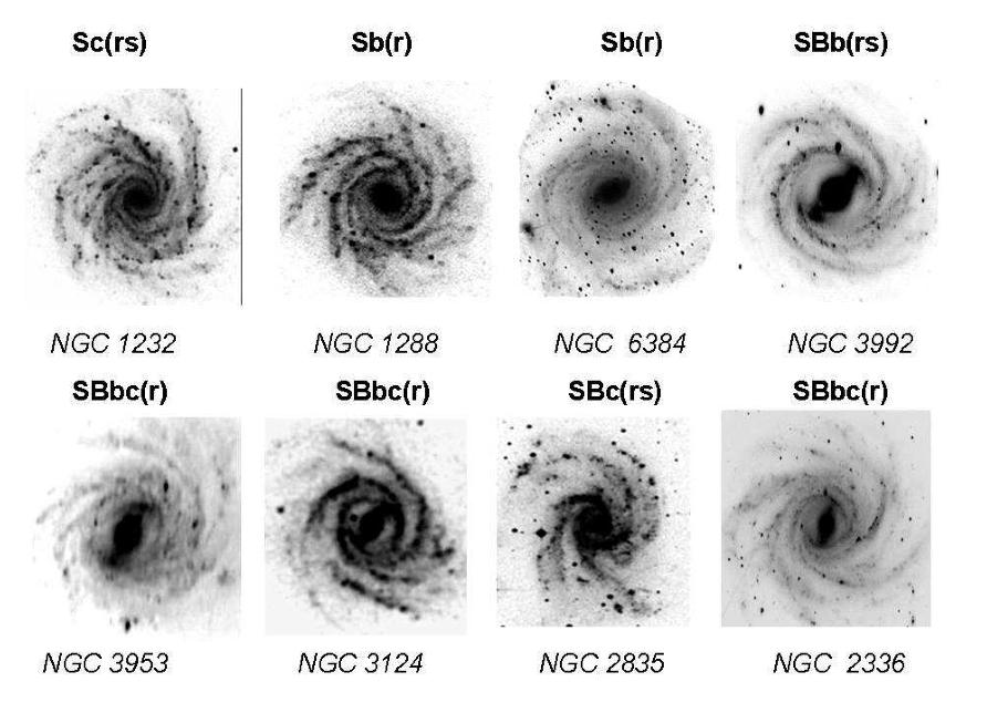
It is clear from Fig. 3 that the Milky Way is a very luminous, reddish galaxy, somewhat at odds with its traditional classification as an SbSbc galaxy. This has raised questions in the past about where it falls on the Tully-Fisher relation (e.g., Malhotra et al., 1996; Hammer et al., 2012). But this high luminosity is consistent with its high circular velocity ( km s-1) discussed in §6.4. In Table 2, the Galaxy is slightly fainter in absolute magnitude and slightly less massive in both stellar and baryonic mass than the average for its rotation speed. When considering both the current uncertainties in Milky Way properties and the scatter of galaxies about the relation, the Galaxy is consistent with the Tully-Fisher relation to better than uncertainty. The Milky Way appears to be a kinematically typical spiral galaxy for its intrinsic luminosity.
3 Galactic Center
3.1 Location
The Galactic Center, as we understand it today, was first identified through the discovery of Sgr A by radio astronomers (Piddington & Minnett, 1951). Based on its unique radio emission properties and its precise coincidence with the dynamical center of the rotating inner H disk (Oort & Rougoor, 1960), the IAU officially adopted Sgr A as the center of the Galaxy, making its position the zero of longitude and latitude in a new system of Galactic coordinates (Blaauw et al., 1959). Later Balick & Brown (1974) discovered the unresolved source Sgr A∗, now known to be at the location of the Milky Way’s supermassive black hole, at (Reid & Brunthaler, 2004).
Thirty years ago, Kerr & Lynden-Bell (1986) gave this working definition of the Galactic Center: Currently it is assumed that the Galactic Centre coincides sufficiently well with the Galaxy’s barycentre that a distinction between the point of greatest star density (or any other central singularity) and the barycentre (centre of mass) is not necessary. It is also assumed that to sufficient accuracy for the internal dynamics of the Galaxy, the Galactic Centre defines an inertial coordinate system. These assumptions could prove to be untrue if for instance the centre of the distribution of the mysterious mass in the heavy halo were displaced from the mass centre of the visible Galaxy.
Indeed, in a hierarchical universe the first assumption is almost certainly violated beyond tens of kpc: we will see in § 6 that the Galaxy continues to accrete satellite galaxies carrying both stars and dark matter; furthermore, the Milky Way’s dark matter halo interacts both with infalling dark matter and with other halos in the Local Group. However, as discussed below, the inner Milky Way appears to have “settled down” to a well-defined and well-centered midplane; thus we may assume that the region of greatest star density coincides with the barycenter of the mass within the Solar Circle.
The second part of the definition may ultimately also come into question. Numerical simulations reveal that dark matter halos tumble at the level of a few radians per Hubble time. The baryonic components are largely bound to the dark matter but may slosh around within them. Furthermore, the spin axis of the Galactic Plane is likely to precess with respect to a celestial coordinate frame defined by distant quasars or radio sources. Over the lifetime of the gaia mission, this precession (as yr-1) should be detectable (Perryman, Spergel & Lindegren, 2014).
Galactic CenterLocation of radio source Sgr A∗ \entry, Galactic coordinates of Sgr A∗ \entrySMBHMilky Way’s supermassive black hole
3.2 Distance
The distance of the Sun to the Galactic Center, , is one of the fundamental scaling parameters for the Galaxy. All distances determined from angular sizes or from radial velocities and a rotation model are proportional to . Also the sizes, luminosities, and masses of objects such as molecular clouds scale with , as do most estimates of global Galactic luminosity and mass. Because is one of the key parameters, we consider its measured value in some detail here. Previous reviews on this subject can be found in Kerr & Lynden-Bell (1986); Reid (1993); Genzel, Eisenhauer & Gillessen (2010); Gillessen et al. (2013), and a recent compilation of results is given in Malkin (2013).
Similar to their discussion, we divide methods of determining into direct (primary), model-based, and secondary. Direct methods compare an angular dimension or velocity near the Galactic Center with a physical length scale or radial velocity (RV), with minimal modelling assumptions and without having to use additional calibrations. Model-based methods determine as one of the model parameters through a global fit to a set of data. Secondary methods finally use standard candle tracers whose distances are based on secondary calibrations such as period-stellar luminosity relations, and whose distributions are known or assumed to be symmetric with respect to the Galactic Center. In the following, we briefly review the different methods. Table 3 gives the list of independent recent determinations of which we use for obtaining an overall best estimate below.
3.2.1 Direct estimates
As discussed more fully in §§3.4, 6.4, the SMBH is at rest at the dynamical center of the Milky Way within the uncertainties (Reid & Brunthaler, 2004; Reid, 2008). Thus can be determined by measuring the distance to the SMBH’s radiative counterpart, Sgr A∗. At distance, the expected parallax of Sgr A∗ is . This would be resolvable with Very Long Baseline Interferometry (vlbi), but unfortunately the image of Sgr A∗ is broadened by interstellar scattering (e.g., Bower et al., 2004). However, Reid et al. (2009b) measured trigonometric parallaxes of H2O masers in Sgr B2, a molecular cloud complex which they estimated is located in front of Sgr A∗.
A second direct estimate of the distance to the SMBH comes from monitoring proper motions (PM) and line-of-sight (LOS) velocities for stellar orbits near Sgr A∗ (Eisenhauer et al., 2003; Ghez et al., 2008; Gillessen et al., 2009b; Morris, Meyer & Ghez, 2012), in particular the star S2 which by now has been followed for a complete orbit around the dynamical center. The main systematic uncertainties are source confusion, tying the SMBH to the astrometric reference frame, and the potential model; relativistic orbit corrections lead to an increase of by (Genzel, Eisenhauer & Gillessen, 2010). See also Gillessen et al. (2009a) who combined the existing two major data sets in a joint analysis.
The statistical parallax of the nuclear star cluster (NSC) obtained by comparing stellar PM and LOS has been used as a third direct estimate of (Genzel et al., 2000; Trippe et al., 2008; Do et al., 2013). This method has now become accurate enough that projection and finite field-of-view effects in combination with orbital anisotropies need to be modelled (Chatzopoulos et al., 2015).
3.2.2 Model-based estimates
vlbi astrometry has provided accurate parallaxes and proper motions for over OH, SiO, and Methanol masers in High Mass Star Formation Regions (HMSFR) in the Galactic disk (Honma et al., 2007, 2012; Reid et al., 2009a, 2014; Sato et al., 2010). Most of these sources are located in the Galactic spiral arms. By fitting a spiral arm model together with a model for Galactic circular rotation to the positions and velocities of the HMSFR, precise estimates of can be obtained together with rotation curve and other parameters (for a different analysis, see Bajkova & Bobylev, 2015). Because distances are determined geometrically, no assumptions on tracer luminosities or extinction are necessary. The main remaining systematic uncertainties thus are the assumption of axisymmetric rotation, the detailed parametrisation of the rotation curve model, and the treatment of outliers.
Another long-standing approach is based on analyzing the velocity field near the Solar Circle, using PM and LOS velocities of various tracers. These methods assume an axisymmetric velocity field and, in some cases, include the perturbing effects of a spiral arm model. In the traditional form, the data are used to solve for the Oort constants A, B (§6.4) from the PMs and for from the RVs, to finally estimate (Mihalas & Binney, 1981; Zhu & Shen, 2013). Another variant is to use young stars or star formation regions assumed to follow circular orbits precisely (Sofue et al., 2011; Bobylev, 2013). An analysis less sensitive to the uncertain perturbations from spiral arms and other substructure is that by Schönrich (2012), who uses a large number of stars with PMs and RVs from the segue survey (Yanny et al., 2009), to determine by combining the rotation signals in the radial and azimuthal velocities for stars within several kpc from the Sun.
A promising new method is based on the detailed dynamical modelling of halo streams. While stream modelling has mostly been used to obtain estimates for the mass and shape of the dark matter halo (see § 6.3), Küpper et al. (2015) showed that with accurate modelling can also be well-constrained as part of a multi-parameter fit to detailed density and LOS velocity measurements along the stream.
Vanhollebeke, Groenewegen & Girardi (2009) compared predictions from a stellar population model for the Galactic bulge and intervening disk to the observed star counts. They used a density model based on NIR data from Binney, Gerhard & Spergel (1997) and varied the star formation history and metallicity distribution of bulge stars. The value of from their best fitting models depends heavily on the magnitudes of red clump stars, showing a close connection to secondary methods.
| Label | Reference | Method | Loc | T | [kpc] |
|---|---|---|---|---|---|
| Rd+09 | Reid et al. 2009 | Trig. Parallax of Sgr B | GC | d | |
| Mo+12 | Morris et al. 2012 | Orbit of S0-2 around Sgr A* | GC | d | |
| Gi+09 | Gillessen et al. 2009 | Stellar orbits around Sgr A* | GC | d | |
| Ch+15 | Chatzopoulos et al. 2015 | NSC statistical parallax | GC | d | |
| Do+13 | Do et al. 2013 | NSC statistical parallax | GC | d | |
| BB15 | Bajkova & Bobylev 2015 | Trig. Parallaxes of HMSFRs | DSN | m | |
| Rd+14 | Reid et al. 2014 | Trig. Parallaxes of HMSFRs | DSN | m | |
| Ho+12 | Honma et al. 2012 | Trig. Parallaxes of HMSFRs | DSN | m | |
| ZS13 | Zhu & Shen 2013 | Near-R0 rotation yg tracers | DSN | m | |
| Bo13 | Bobylev 2013 | Near-R0 rotation SFRs+Cephs | DSN | m | |
| Sch12 | Schönrich 2012 | Near-R0 rotation SEGUE stars | DSN | m | |
| Ku+15 | Küpper et al. 2015 | Tidal tails of Pal-5 | IH | m | |
| VH+09 | Vanhollebeke et al. 2009 | Bulge stellar popul. model | B | m | |
| Pi+15 | Pietrukowicz et al. 2015 | Bulge RR Lyrae stars | B | s | |
| De+13 | Dekany et al. 2013 | Bulge RR Lyrae stars | B | s | |
| Da09 | Dambis 2009 | Disk/Halo RR Lyrae stars | DSN | s | |
| Ma+13 | Matsunaga et al. 2013 | Nuclear bulge T-II Cepheids | B | s | |
| Ma+11 | Matsunaga et al. 2011 | Nuclear bulge Cepheids | B | s | |
| Gr+08 | Groenewegen et al. 2008 | Bulge Cepheids | B | s | |
| Ma+09 | Matsunaga et al. 2009 | Bulge Mirae | B | s | |
| GrB05 | Groenewegen & Bl. 2005 | Bulge Mirae | B | s | |
| FA14 | Francis & Anderson 2014 | Bulge red clump giants | B | s | |
| Ca+13 | Cao et al. 2013 | Bulge red clump giants | B | s | |
| Fr+11 | Fritz et al. 2011 | NSC red clump giants | GC | s | |
| FA14 | Francis & Anderson 2014 | All globular clusters | BIH | s | |
| Bi+06 | Bica et al. 2006 | Halo globular clusters | IH | s |
Recent determinations of the distance to the Galactic Center, , used for weighted averages and in Fig. 4. Columns give label for Fig. 4, reference, location (Galactic Center, bulge, disk and solarneighbourhood, inner halo), type of measurement (direct, model-based, secondary), . The listed uncertainties include statistical and systematic errors, added in quadrature when both are published. Where a systematic error is not quoted by the authors or included in their total published error, we estimated it from results obtained by them under different assumptions, when possible (GrB05, Fr+11, BB15, Rd+14, Bo13, Bi+06). For Ca+13 who did not give an error, we estimated one from the metallicity dependence of the RCG calibration of Nataf et al. (2013). In the remaining cases (ZS13, Sch12, Kue+15, Da09) we took the systematic error to be equal to the statistical error.
3.2.3 Secondary estimates
There is a long history of secondary measurements based on the distance distributions of RR Lyrae stars, Cepheids, Mira stars, red clump giants (RCG), and globular clusters (Reid, 1993). Individual distances are derived from external calibrations of period-luminosity (PL) relations for the variable stars, and from horizontal branch (HB) magnitudes for RCG and globular clusters. The main systematic errors in these methods come from uncertainties in the calibrations, but also from the extinction corrections and reddening law, and from how the distance distribution in the survey volume is related to the center of the Galaxy.
RR Lyrae, pulsationally unstable HB stars with characteristic absolute magnitudes , (Catelan, Pritzl & Smith, 2004), are the primary distance tracers for old, metal-poor populations. Large numbers of RR Lyrae stars identified by the ogle (Udalski et al., 2008) and vvv surveys (Minniti et al., 2010) were recently used to map out the old metal-poor population in the bulge (Pietrukowicz et al., 2015; Dékány et al., 2013, respectively). Individual distances are more accurate by a factor in the NIR than in optical data, due to higher precision and reduced metallicity dependence in the PL-relation, and less sensitivity to reddening. With the large bulge samples the centroid of the distribution can be determined more accurately than in earlier work (e.g., Groenewegen, Udalski & Bono, 2008; Majaess, 2010). On larger Galactic scales, Dambis (2009) calibrated thick disk and halo RR Lyrae populations separately by statistical parallax to then estimate .
Type II Cepheids trace old, typically metal-poor populations; they are brighter than RR Lyrae stars but much less numerous. Groenewegen, Udalski & Bono (2008) used NIR data for 39 population II Cepheids in the bulge from the ogle survey; a related work is by Majaess (2010). Matsunaga et al. (2011, 2013) analysed 3 classical Cepheids and 16 type II Cepheids from a NIR survey of the inner in the nuclear bulge.
Groenewegen & Blommaert (2005) obtained a PL relation for 2691 Mira long period variables in the ogle bulge fields while Matsunaga et al. (2009) studied 100 Miras in the nuclear bulge. For these red giants the extinction corrections are smaller, but calibrations from the Large Magellanic Cloud (LMC) and globular clusters were needed to estimate from these data.
Since the work of Paczynski & Stanek (1998), red clump giants (RCG) have been recognized as important distance probes in the Galaxy (see Girardi, this volume). RCG are He-core burning stars with a narrow range of luminosities, especially in medium-to-old age populations such as in the Galactic bulge. Typical absolute magnitudes are , , with a dispersion - mag, and systematic effects due to age and metallicity variations are relatively small and fairly well understood. Surveys towards the inner Galaxy are frequently done in the NIR to minimize extinction (Babusiaux & Gilmore, 2005; Nishiyama et al., 2006) or in the -band (Paczynski & Stanek, 1998; Nataf et al., 2013). The -band studies tend to give slightly shorter distances. Fritz et al. (2011) used RCG in several NIR bands to determine a distance to the central NSC.
The centroid of the distance distribution of globular clusters, the basis for the famous early work by Shapley (1918), continues to be used for estimating (Bica et al., 2006; Francis & Anderson, 2014). These studies are based on the catalogue of Harris (2010, and earlier), where individual distances are estimated from HB magnitudes and reddening. The distance distribution of the clusters is somewhat asymmetric, and values found are on the low side of the distribution in Table 3. Systematic effects could be due to missing clusters behind the Galactic Center, or to errors in the HB magnitudes, e.g., from extinction uncertainties or stellar confusion in crowded cluster fields (Genzel, Eisenhauer & Gillessen, 2010). However, the method provides a rare opportunity to estimate from Galactic halo tracers.
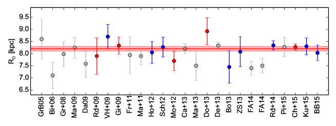
3.2.4 Overall best estimate and discussion
Table 3 gives the list of recent determinations which we use for obtaining an overall best estimate for . For each method we kept at most three determinations to prevent overweighting often-employed techniques with similar systematic uncertainties; for example, there are many determinations of using RCG as standard candles. We omitted determinations which were later updated by the same group of authors based on improved data, but kept independent reanalyses of published data by other authors. We also did not include estimates which used priors based on measured values already taken into account (e.g. McMillan, 2011).
Fig. 4 shows the overall distribution of these measurements with time, and the separate distributions for tracers in the Galactic Center, bulge, disk, and halo, respectively. To obtain a best estimate for , we consider weighted means for the total and various subsamples. For any measurements, we compute (i) the standard error of the weighted mean, SE; (ii) the unbiassed standard error of the weighted mean (UE, square root of times the unbiassed weighted sample variance); (iii) following Reid (1993), we consider possible correlations between some of the measurements. These can arise, e.g., because HB or PL calibrations use very similar theoretical models or calibrators, or are based on a common LMC distance; because two data sets, although independent, can only be obtained for the same small number of stars; or because several measurements are all based on the assumption that the velocity field near the Solar Circle is axisymmetric. Clearly, some of these correlations have stronger influence than others. For a conservative error evaluation, we retain independent measurements for the total sample, and for the separate (GC, B, DSN, IH) tracer samples. We note that the sets of methods kept for the different regions are largely independent. In each case, we determine a UUE uncorrelated sample error by replacing in UE by .
Using the notation , we find for the total sample; for measurements 2013 or later; for the 4 measurements with errors (Ch+15, Rd+14, De+13, Ca+13); for the 11 uncorrelated best determinations; excluding the values outside their of the overall weighted mean; and for all values excluding halo. All data samples give very consistent results; the fact that SE and UE generally agree within suggests that the errors given for the individual measurements are mostly realistic. Based on the scatter and UUE errors of the various sample means, we adopt here our best estimate for the distance to the Galactic Center: . This value is significantly lower than the IAU standard ().
The weighted sample means for tracers in the different regions of the Galaxy are for the GC sample, for the B sample, for the DSN sample, and for the IH sample. The fact that tracers in the Galactic Center, bulge, and disk result in similar estimates for within small errors (also for UUE with largely independent respective methods) suggests that the different Galactic components are well-centered, and thus that relative sloshing motions between these components must currently be unimportant. Together with the good alignment of the Milky Way bar and H disk with the Galactic plane (§ 3.3), this suggests that the inner Milky Way has settled to a well-determined equilibrium state. Even the inner halo tracers on scales of are consistent with having the same Galactic Center as the bulge and disk, within error.
We anticipate significant improvements in many of these distance measurements based on data from the gaia satellite, which will provide accurate parallaxes and proper motions for large numbers of Milky Way stars. These data will greatly improve our dynamical understanding of the Galactic disk, but also of the bulge and bar outside highly extincted regions, and lead to much-improved secondary calibrations, e.g., for RR Lyrae and RCG. The direct estimate of from stellar orbits around Sgr A∗ is expected to improve steadily as the time base line increases and more orbits can be reliably constrained, and especially with accurate astrometric and spectroscopic monitoring of the next close pericenter passage (2018 for the star S2).
, Sun’s distance from Galactic Center \entry, solar offset from local disk midplane
3.3 Solar offset and Galactic plane
Early estimates of the Sun’s vertical position with respect to the Galactic Plane date back to van Tulder (1942)’s analysis of stellar catalogues, from which was determined pc towards the North Galactic pole. In support of the early value, Conti & Vacca (1990) obtained pc using Wolf-Rayet stars within 20 kpc of the Sun. pioneer 10 observations of the optical background light in the Galaxy indicated pc (Toller, 1990), and modeling the cobe NIR surface brightness distribution resulted in pc (Binney, Gerhard & Spergel, 1997).
But more expansive studies of the nearby disk show that these are underestimates. Chen et al. (2001) demonstrated the importance of correctly treating the larger-scale parameters of the disk population in such studies, using the sdss photometric survey. While the radial scalelength is relatively unimportant, a vertically extended population with a well established scaleheight is critical. The following estimates are based on either OB stars, open clusters, or optical star counts for a range of stellar populations, and are broadly consistent: pc (Stothers & Frogel, 1974); pc (Pandey, Bhatt & Mahra, 1988); pc (Humphreys & Larsen, 1995); pc (Mendez & van Altena, 1998); pc (Chen et al., 1999); pc (Chen et al., 2001); pc (Maíz-Apellániz, 2001). While the last estimate from hipparcos OB stars has the smallest error, the distribution of young stars may be more sensitive to various perturbations, as illustrated by Gould’s belt. Therefore we adopt here the best estimate from the complete sdss photometric survey, i.e. pc (Jurić et al., 2008), which captures all these values.
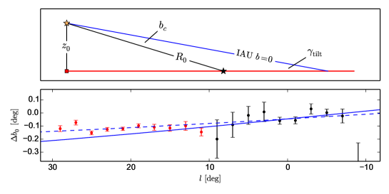
The Galactic midplane was defined based on the very flat distribution of H gas in the inner Galaxy, with an estimated uncertainty in the position of the Galactic pole of (Blaauw et al., 1960). Because the Sun was found to lie in the H principal plane within the errors, and the measured offset relative to Population I stars was not considered reliable, the plane was defined to pass through the Sun and Sgr A (not Sgr A∗). Since we know now that , the true Galactic plane is likely to be slightly inclined relative to the plane . If it is assumed that Sgr A∗ lies precisely in the Galactic plane (see § 3.4), the required inclination angle is (see Fig. 5 and Goodman et al., 2014). Objects located in the Galactic plane between the Sun and the Galactic Center then appear at slightly negative latitudes. Near-infrared star counts in the inner Galaxy have enough signal-to-noise to detect such offsets. The mean latitude of the peak of RCG counts in the Galactic long bar (see § 4.3) is indeed found at , corresponding to an offset of at distance (Wegg, Gerhard & Portail, 2015). The observed peak latitudes agree with those predicted for the inclined plane to within or of the half-length of the bar (Fig. 5). The Galactic long bar is thus consistent with lying in a tilted midplane passing through Sgr A∗ and the point below the Sun to within . Both stars and H gas suggest that the Galactic disk inside the Solar Circle is very nearly flat.
3.4 Black hole and solar angular velocity
Measurements in the Milky Way have provided the best evidence for a central SMBH to date; see Reid (2009) and Genzel, Eisenhauer & Gillessen (2010) for recent reviews. Infrared studies of the motions of gas clouds in the Sgr A region first indicated a central point mass of several (e.g., Lacy et al., 1980). Later, PM measurements of stars in the dense NSC showed evidence for a Keplerian increase of the stellar velocity dispersion to several at of the Galactic Center, corresponding to a central mass of (Eckart & Genzel, 1997; Ghez et al., 1998). Currently, from accurate LOS velocities and astrometric measurements with adaptive optics, stellar orbits have been determined for some 30 of the so-called S-stars in the central arcsec, including one complete 15.8 year orbit for the star S2. All orbits are well-fitted by a common enclosed mass and elliptical orbit focal point. From multi-orbit fits, rescaled to , the total enclosed mass is (Ghez et al., 2008) and (Gillessen et al., 2009b), and from a joint analysis of the combined VLT and Keck data (Gillessen et al., 2009a). The error given is combined statistical and systematic and is expected to improve steadily with increasing time baseline of the measurements; it has an important contribution from a degeneracy between and .
Therefore, external constraints on reduce the range of black hole mass allowed by the orbit measurements. Combining with their measurement of the NSC statistical parallax, Chatzopoulos et al. (2015) found . Using instead the overall best from §3.2, the mass of the black hole becomes . This corresponds to a Schwarzschild radius of , and to a dynamical radius of influence , where the interior mass of the NSC (Chatzopoulos et al., 2015). The inferred mass is also consistent with the orbital roulette value obtained by Beloborodov et al. (2006) from the stellar motions in the clockwise disk of young stars around Sgr A∗. For and a bulge velocity dispersion of (§4.2.3), the Milky Way falls below the best-fitting relation for elliptical galaxies and classical bulges by a factor of - (Kormendy & Ho, 2013; Saglia et al., 2016).
, mass of Galactic SMBH \entry, mass density within pericenter of star S2 \entry, SMBH’s dynamical influence radius
From the orbit fit, any extended mass distribution within the orbit of S2 can contribute no more than of the enclosed mass. The S2 star has approached the central mass within at pericenter, requiring a minimum interior mass density of . This is so large that one can rule out any known form of compact object other than a black hole (Reid, 2009; Genzel, Eisenhauer & Gillessen, 2010). From matching the positions of SiO maser stars visible both in the NIR and the radio, the position of the compact mass and the radio source Sgr A∗ have been shown to coincide within (Reid et al., 2003; Gillessen et al., 2009b). The size of Sgr A∗ in radio observations is (Shen et al., 2005; Doeleman et al., 2008). These facts taken together make it highly likely that Sgr A∗ is the radiative counterpart of the black hole at the center of the Galaxy.
The apparent PM of Sgr A∗ relative to a distant quasar (J1745-283) has been measured with great precision using vlbi (Reid & Brunthaler, 2004; Reid, 2008). The PM perpendicular to the Galactic plane is entirely consistent with the reflex motion of the vertical peculiar velocity of the Sun, with residual , suggesting strongly that the SMBH is essentially at rest at the Galactic Center. Indeed the Brownian motion of the SMBH due to perturbations from the stars orbiting inside its gravitational influence radius is expected to be (Merritt, Berczik & Laun, 2007). On the assumption that Sgr A∗ is motionless at the Galactic Center, its measured PM in the Galactic plane determines the total angular velocity of the Sun with high accuracy: . For from §3.2, the inferred value of the total solar tangential velocity relative to the Galactic Center is . We will return to these constraints in our discussion of the Galactic rotation curve in §6.4 which brings together many of the major themes of this review.
Sun’s total angular velocity relative to Sgr A∗ \entry , Sun’s tangential velocity relative to Sgr A∗
4 Inner Galaxy
4.1 Nuclear star cluster and stellar disk
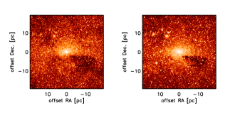
Becklin & Neugebauer (1968) discovered an extended NIR source centered on Sgr A: the MW’s nuclear star cluster (NSC). The source had a diameter of , was elongated along the Galactic plane, and its surface brightness fell with projected radius on the sky . NSC are commonly seen in the centers of disk galaxies and many contain an AGN and thus a SMBH (e.g. Böker, 2010). NIR spectroscopy has shown that most of the luminous stars in the Galactic NSC are old () late-type giant and RCG stars (the “old” NSC, Pfuhl et al., 2011). But also a surprising number of massive early-type stars were found in this volume (Krabbe et al., 1995), including massive young stars in one and possibly two disks with diameters rotating around the SMBH (Paumard et al., 2006; Bartko et al., 2009), and a remarkable concentration of B-stars within of the SMBH, the so-called S-stars (Eckart et al., 1995). Recent reviews on the NSC can be found in Genzel, Eisenhauer & Gillessen (2010) and Schödel et al. (2014b).
The structure and dynamics of the NSC must be studied in the IR because of the very high extinction towards the GC ( mag, mag, Fritz et al., 2011; Nishiyama et al., 2008). Recent analysis of spitzer/IRAC images (Schödel et al., 2014a) has shown that the old NSC is centered on Sgr A∗ and point-symmetric, and it is flattened along to the Galactic plane with minor-to-major projected axis ratio . Chatzopoulos et al. (2015) obtain from fitting K-band star counts; they also show that NSC dynamics requires a flattened star cluster with an axis ratio consistent with this value. The NSC radial density profile is discussed in these papers and in Fritz et al. (2016). When fitting the data with a Sersic profile, Schödel et al. (2014a) obtain a total luminosity and a spherical half-light radius of .
NSCNuclear star cluster \entry , NSC Luminosity \entry, half-light radius \entry , axis ratio \entry , NSC mass
The dynamical mass within is (Chatzopoulos et al., 2015); thus and the total mass of the NSC for the Sersic model is . An additional error in not accounted for in this estimate comes from the fact that the surface density profile of the NSC goes below that of the much larger, surrounding nuclear stellar disk at projected , making its outer density profile uncertain (Chatzopoulos et al., 2015). The rotation properties and velocity dispersions were measured by Trippe et al. (2008); Fritz et al. (2016) from stellar PM and LOS velocities, and from NIR integrated spectra by Feldmeier et al. (2014). The NSC is approximately described by an isotropic rotator model, with slightly slower rotation (Chatzopoulos et al., 2015). There are indications for a local kinematic misalignment in the LOS velocities but not in the PM (Feldmeier et al., 2014; Fritz et al., 2016) which, if confirmed, might indicate some contribution to the NSC mass by infalling star clusters (Antonini et al., 2012); this needs further study. Another unsolved problem is the apparent core in the NSC density profile (Buchholz, Schödel & Eckart, 2009); this might indicate that the NSC is not fully relaxed, consistent with the relaxation time estimated as throughout the NSC (Merritt, 2013).
The old NSC is embedded in a nuclear stellar disk (NSD) which dominates the three-dimensional stellar mass distribution outside (Chatzopoulos et al., 2015) and within (Launhardt, Zylka & Mezger, 2002). From star counts, its vertical density profile is near-exponential with scale-height (Nishiyama et al., 2013). This confirms an earlier analysis of cobe data by Launhardt, Zylka & Mezger (2002) which cover a larger area but with lower resolution. The projected density profile along the major axis () is approximately a power-law out to ; thereafter it drops steeply towards the NSD’s outer edge at , approximately . The axis ratio of the NSD inferred in these papers from the star counts and NIR data is 3:1 at small radii and 5:1 on the largest scale. The total stellar mass estimated by Launhardt, Zylka & Mezger (2002) is , of order 10% of the mass of the bulge. The rotation of the NSD has been seen in OH/IR stars and SiO masers (Lindqvist, Habing & Winnberg, 1992; Habing et al., 2006) and with apogee stars (Schönrich, Aumer & Sale, 2015), with an observed gradient and estimated rotation velocity at . These data suggest a dynamical mass on the lower side of the estimated stellar mass range. The NSD is likely related to past star formation in the zone of -orbits near the center of the barred potential (e.g. Molinari et al., 2011). Clearly, understanding the NSD better is relevant for the evolution of the Galactic bulge and probably also for the growth of the SMBH, and further information about its kinematics and stellar population would be important. Figure 6 illustrates this still enigmatic Galactic component together with the NSC.
NSDNuclear stellar disk \entry, NSD break radius \entry, NSD vertical scale-height \entry, stellar mass of NSD
4.2 Bulge
For many years, the Galactic bulge was considered as a structure built through mergers early in the formation of the Galaxy, now called a classical bulge. Particularly the old ages of bulge stars inferred from color-magnitude diagrams supported this view (Ortolani et al., 1995; Clarkson et al., 2008). The NIR photometry with the dirbe instrument on board the cobe satellite first established the boxy nature of the bulge (Weiland et al., 1994; Binney, Gerhard & Spergel, 1997), later confirmed by the 2mass star count map (Skrutskie et al., 2006). Recent star count data have unambiguously established that the bulk of the bulge stars are part of a so-called box/peanut or b/p-bulge structure representing the inner, three-dimensional part of the Galactic bar (McWilliam & Zoccali, 2010; Nataf et al., 2010; Wegg & Gerhard, 2013), consistent with the observed cylindrical rotation (Kunder et al., 2012; Ness et al., 2013b). This corroborates long-standing evidence for a barred potential in the bulge region from non-circular motions seen in H and CO longitude-velocity-()-diagrams (Binney et al., 1991; Englmaier & Gerhard, 1999). The central parts of the Galaxy also contain the dense NSD and some have argued for a separate, -scale nuclear bar (Alard, 2001; Rodriguez-Fernandez & Combes, 2008). Finally, the peak in the density of the inner stellar halo is found in this region as well. Disentangling these various components clearly requires the best data possible. Results to date and open issues are summarized below. More extensive reviews of the Galactic bulge can be found in Rich (2013); Gonzalez & Gadotti (2016); Shen & Li (2015).
4.2.1 The Galactic b/p bulge
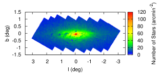
A large fraction of the bulge stars follows a rotating, barred, box/peanut shaped bulge with exponential density distribution, similar to the inner three-dimensional part of an evolved N-body bar. The best available structural information for the dominant bulge population comes from large samples of red clump giant stars (RCG), for which individual distances can be determined to accuracy. These He-core burning stars have a narrow range of absolute magnitudes and colors, and and are predicted to trace the stellar population within for metallicities in the range [0.02,1.5] solar (Salaris & Girardi, 2002). In the color-magnitude diagram, RCG appear spread because of distance, reddening, age ( in Ks at age ), and metallicity (by for the measured bulge metallicity distribution). Among the 25,500 stars of the argos survey, RCG are prominent down to [Fe/H], which comprises of their sample (Ness et al., 2013a); i.e., RCG are representative for most of the bulge stars.
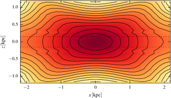
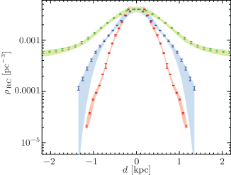
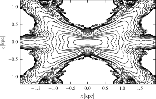
Using million RCG from the vvv survey (Minniti et al., 2010) over the region , , Wegg & Gerhard (2013) obtained RCG line-of-sight density distributions for sightlines outside the most crowded region , and combined these to a 3-dimensional map of the bulge RCG density assuming 8-fold triaxial symmetry (Figure 7). As shown in the figure, rms variations between 8-fold symmetric points in the final map are indeed small; there is no evidence for asymmetries in the volume of the RCG measurement (). The RCG bulge is strongly barred, with face-on projected axis ratio for isophotes reaching along the major axis; it has a strong b/p-shape viewed side-on, and a boxy shape as seen from the Sun, consistent with the earlier cobe and 2mass data. Unsharp masking (Portail et al., 2015) results in a strong off-centered X-shape structure (Fig. 7), similar to some galaxies in the sample of Bureau et al. (2006); see also Nataf et al. (2015).
The near side of the b/p bulge has its major axis in the first Galactic quadrant (). The bar angle between major axis and the Sun-Galactic center line found by Wegg & Gerhard (2013) is , with most of the error systematic. This is consistent with earlier parametric determinations from ogle band RCG star counts (, Cao et al., 2013), (, Rattenbury et al., 2007), (, Stanek et al., 1997), from non-parametric inversion of 2mass red giant star counts (, López-Corredoira, Cabrera-Lavers & Gerhard, 2005), and from modelling the asymmetry of the cobe NIR photometry (, Dwek et al., 1995; Binney, Gerhard & Spergel, 1997; Freudenreich, 1998; Bissantz & Gerhard, 2002). The global bulge axis ratios obtained with parametric star count models are typically , similarly to those found from modelling the cobe data. However, it is clear from Fig. 7 that a single vertical axis ratio does not capture the shape of the b/p bulge. The lower left panel shows that the density distributions inside are nearly exponential, with scale-lengths and axis ratios (Wegg & Gerhard, 2013). Further down the major axis, increases to at where the X-shape is maximal, and then decreases rapidly outwards.
Box/Peanut (b/p) bulge \entry , b/p bulge bar angle \entry , axis ratio from top \entry , edge-on axis ratio \entry , vertical scale-height \entry , radius of max. X
4.2.2 Inner bulge and disk structure
The structure of the inner Galactic disk between the NSD and is not well-known due to heavy extinction and crowding. Observations of maser stars and vvv Cepheids indicate a barred disk of young stars (Habing et al., 2006; Dékány et al., 2015). The cold kinematics of young bar stars has likely been seen in apogee LOS velocity histograms (Aumer & Schönrich, 2015). The short vertical scale height in the bulge is perhaps indicative of a central disk-like, high-density pseudo-bulge structure, as is seen in many early and late type b/p bulge galaxies (Bureau et al., 2006; Kormendy & Barentine, 2010). NIR RCG star counts at have confirmed a structural change in the RCG longitude profiles at (Nishiyama et al., 2005; Gonzalez et al., 2011a; Wegg & Gerhard, 2013). This has been interpreted by means of an N-body model in terms of a rounder, more nearly axisymmetric central parts of the b/p bulge (Gerhard & Martinez-Valpuesta, 2012). As predicted by the model, the transition at is confined to a few degrees from the Galactic plane (Gonzalez et al., 2012).
The nuclear bulge within is dominated by the NSD. Based on longitudinal asymmetries in a map of projected 2mass star counts Alard (2001) presented indications for a scale nuclear bar separate from the b/p bulge-bar. However, the large-scale Galactic bar by itself leads to similar inverted asymmetries in the center, just by projection (Gerhard & Martinez-Valpuesta, 2012), so the observed asymmetries are not a tell-tale signature. Unfortunately, the distance resolution of the RCG is not sufficient to investigate the LOS-structure of a tilted nuclear bar. Thus the most promising test appears to be with models of the nuclear gas flow (Rodriguez-Fernandez & Combes, 2008), but this requires understanding the larger-scale properties of the gas flow better (see §4.4) which influence the nuclear gas flow. Further studies in the IR, both photometric and spectroscopic, are clearly needed to shed more light on the inner bulge.
4.2.3 Does the Milky Way have a classical bulge? Kinematics and metallicities of bulge stars
Bulges in several disk galaxy formation models have been found to harbour a rapid early starburst component, as well as a second component which forms later after disk build-up and instabilities, and/or minor mergers (Samland & Gerhard, 2003; Obreja et al., 2013). The former could be associated with a classical bulge even in the absence of a significant early merger-built bulge. The Milky Way bulge has a well-established vertical metallicity gradient (Zoccali et al., 2008; Johnson et al., 2011; Gonzalez et al., 2013) which has often been taken as the signature of a dissipatively formed classical bulge (see Pipino, Matteucci & D’Ercole, 2008). However, because violent relaxation is inefficient during the bar and buckling instabilities, preexisting metallicity gradients, such that stars with lower binding energies have lower metallicities, would survive as outward metallicity gradients in the final b/p bulge (Martinez-Valpuesta & Gerhard, 2013; Di Matteo et al., 2014). Recent spectroscopic surveys have attributed the vertical metallicity gradient to a superposition of several metallicity components whose relative contributions change with latitude (Babusiaux et al., 2010; Ness et al., 2013a). Hence the signature of a classical bulge must be found with more detailed kinematic and chemical observations.
The mean line-of-sight rotation velocities of bulge stars are nearly independent of latitude, showing cylindrical rotation as is common in barred bulges. First found with planetary nebulas (Beaulieu et al., 2000), this was shown conclusively with the brava (Kunder et al., 2012), argos (Ness et al., 2013b), and gibs (Zoccali et al., 2014) surveys. Rotation velocities reached at are . LOS velocity dispersions at are at and increase rapidly towards the Galactic plane, reaching in Baade’s window at . Based on the dynamical model of Portail et al. (2015, see §4.2.4), mass-weighted velocity dispersions inside the bulge half mass radius are and the rms is , to .
The argos survey mapped the kinematics for different metallicities, showing that higher/lower metallicity stars have lower/higher velocity dispersions. Soto, Rich & Kuijken (2007) and Babusiaux et al. (2010) found differences between the vertex deviations of metal-rich and metal-poor bulge stars and argue for the existence of two main bulge stellar populations, of which only the more metal-rich one follows the bar. Rojas-Arriagada et al. (2014) find two about equally numerous, metal-rich and metal-poor components in the metallicity distribution of their fields, whereas (Ness et al., 2013a, b) find evidence for five populations. The metal-rich components trace the X-shape and hence the barred bulge, but the origin of the metal-poor stars ([Fe/H]) is currently debated. They could represent an old bulge formed through early mergers, or a thick disk component participating in the instability together with the inner stellar halo (e.g. Babusiaux et al., 2010; Di Matteo et al., 2014).
Large numbers of RR Lyrae stars found in the ogle and vvv bulge surveys have shown that the most metal-poor ([Fe/H] ), old population does not participate in the b/p-bulge (Dékány et al., 2013; Pietrukowicz et al., 2015), consistent with the argos result that only stars with [Fe/H] participate in the split red clump (Ness et al., 2012). The RR Lyrae stars show no significant rotation (Kunder et al., 2016). By contrast, the argos stars with [Fe/H] rotate still fairly rapidly; whether they could be stars from the stellar halo or a low-mass classical bulge spun up by the b/p-bulge (Saha, Martinez-Valpuesta & Gerhard, 2012) or whether they could include a component of thick disk stars must still be checked in detail.
In summary, it is unclear at this time whether the Milky Way contains any classical bulge at all - comparing N-body-simulated b/p bulge models to the brava data, Shen et al. (2010) found that the cylindrical rotation in the Galactic bulge could be matched by their models only if the initial models contained a classical bulge with of the initial disk mass ( of the final bulge mass), and none was needed. However, there is strong evidence from structural and kinematic properties that the major part of the Galactic bulge was built from the disk through evolutionary processes similar to those observed in galaxy evolution simulations, as is also inferred for many external galaxies (so-called secular evolution – Kormendy, 2013; Sellwood, 2014).
4.2.4 Mass and mass-to-light ratio in the bulge
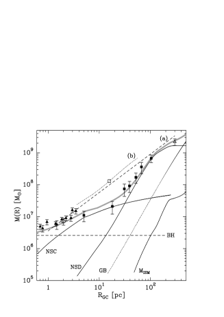
The stellar mass of the bulge can be estimated from a photometric model combined with a stellar population model. For example, Dwek et al. (1995) obtained from the cobe NIR luminosity and a Salpeter IMF ( rescaled for Kroupa IMF, Licquia, Newman & Brinchmann, 2015). Valenti et al. (2016) obtained a projected mass of from scaling the measured mass function in a small bulge field to the whole bulge using RCG. The stellar mass corresponds to the dynamical mass only if the contribution of dark matter in the bulge region is unimportant.
The dynamical mass in the bulge can be determined either from gas kinematics in the bulge region, or from stellar kinematics combined with a dynamical model. For a barred bulge, simple rotation curve analysis does not apply, and analysis of the full gas velocity field requires hydrodynamical models (see §4.4). Stellar-dynamical models require a well-determined tracer density, i.e., a NIR luminosity or tracer density distribution. Furthermore, since the dominant part of the Galactic bulge is the inner b/p part of the Galactic bar, the result depends somewhat on the spatial region defined as “the bulge”.
Zhao, Spergel & Rich (1994) built a self-consistent model of the bar/bulge using the Schwarzschild method, and found a total bulge mass of . Kent (1992) modelled the spacelab emission with an oblate isotropic rotator and constant mass-to-light ratio, finding a mass of . Bissantz, Englmaier & Gerhard (2003) determined the circular velocity at to be , modelling gas dynamics in the potential of the deprojected cobe NIR luminosity distribution from Bissantz & Gerhard (2002). Assuming spherical symmetry, this leads to a total bulge mass of about . However, a number of other studies have found lower masses (Licquia, Newman & Brinchmann, 2015).
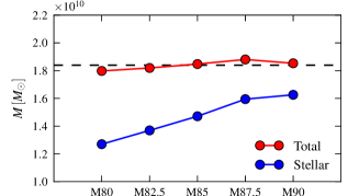
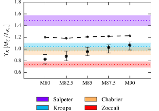
In the most recent study, Portail et al. (2015) find a very well-constrained total dynamical mass of in the vvv bulge region (the box ), by fitting made-to-measure dynamical models to the combined vvv RCG star density and brava kinematics (Figure 8). The data can be fit well by models with a range of dark-to-stellar mass ratios. Comparing the implied total surface mass density with the cobe surface brightness and stellar population models, a Salpeter IMF for a old population can be ruled out, predicting significantly more mass than is dynamically allowed. For an IMF between those of Kroupa (2001); Chabrier (2003); Zoccali et al. (2000), - of the mass in the bulge region would required to be in dark matter. Recently Calamida et al. (2015) derived the bulge IMF in the sweeps field, removing foreground disk stars, and found a double-power law form remarkably similar to a Kroupa or Chabrier IMF. The models of Portail et al. (2015) then predict a total stellar mass in this region of , including stars in the inner disk, and a dark matter fraction of -. The estimated total stellar mass in the bulge and disk of the Galaxy is (§6.4), so the ratio of stellar mass in the bulge region to total is .
, dynamical mass in vvv bulge region \entry, stellar mass in vvv bulge region \entry/, stellar mass in the bulge region to total \entry, dark matter fraction in vvv region \entry km/s, mass-weighted velocity dispersions within half-mass radius along and rms \entry, classical bulge (clb) fraction
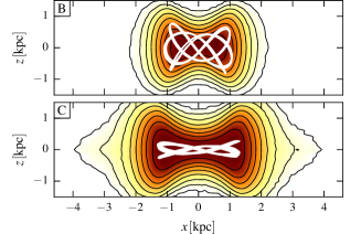
The stellar mass involved in the peanut shape is important for constraining the origin of the bulge populations (§4.2.3). Li & Shen (2012) applied an unsharp masking technique to the side-on projection of the model of Shen et al. (2010), removing an elliptical bulge model from the total. This revealed a centred X-structure accounting for about of their model bulge. Portail et al. (2015) removed a best-matched ellipsoidal density from the three-dimensional RCG bulge density of Wegg & Gerhard (2013), finding that of the bulge stellar mass remained in the residual X-shape. Most reliable would be a dynamical, orbit-based definition of the mass in the peanut shape. However, in the bulge models of Portail et al. (2015), stars in the X-shape do not stream along ‘banana’ orbits (Pfenniger & Friedli, 1991) which follow the arms of the X-shape. Instead, the peanut shape is supported by ‘brezel’ orbit families which contribute density everywhere between the arms of the X-structure (Portail, Wegg & Gerhard, 2015, see Fig. 7). In these models, the fraction of stellar orbits that contribute to the X-structure account for - of the bulge stellar mass.
4.3 The “long bar” outside the bulge
In N-body models for disk galaxy evolution, box/peanut bulges are the inner three-dimensional parts of a longer, planar bar that formed through buckling out of the galaxy plane and/or orbits in vertical resonance (Combes et al., 1990; Raha et al., 1991; Athanassoula, 2005). There is also evidence that b/p bulges in external galaxies are embedded in longer, thinner bars (Bureau et al., 2006). Thus also the Milky Way is expected to have a thin bar component extending well outside the b/p bulge. Finding the Galactic planar bar and characterizing its properties has however proven difficult, because of intervening dust extinction and the superposition with the star-forming disk at low-latitudes towards the inner Galaxy.
Hammersley et al. (2000) drew attention to an overdensity of stars in the Milky Way disk plane reaching outwards from the bulge region to . NIR star count studies with ukidss and other surveys confirmed this structure (Cabrera-Lavers et al., 2007, 2008). Its vertical scale-length was found to be less than , so this is clearly a disk feature. With spitzer glimpse mid-infrared star counts, less affected by dust than K-band data, Benjamin et al. (2005) similarly found a strong bar-like overdensity of sources at positive longitudes. Because of its wide longitude extent and the narrow extent along the LOS this structure was termed the “long bar”.
Based on the combined 2mass, ukidss, vvv, and glimpse surveys, Wegg, Gerhard & Portail (2015) investigated the long bar in a wide area in latitude and longitude, and , using RCG stars and correcting for extinction star-by-star. They found that the Galactic bar extends to at from the Galactic plane, and to at lower latitudes. Their long bar has an angle to the line-of-sight of , consistent with the bar angle inferred for the bulge at . The vertical scale-height of the RCG stars decreases continuously from the b/p bulge to the long bar. Thus the central b/p bulge appears to be the vertical extension of a longer, flatter bar, similar as seen in external galaxies and N-body models.
These recent results are based on a larger and more uniform data base and on a more uniform analysis than the earlier work on the long bar, using cross-checked star-by-star extinction corrections and a statistical rather than CMD-based selection of RCG stars. This leads to smaller errors in the RCG magnitude distributions and reduced scatter between neighbouring fields, particularly near the Galactic plane. These results therefore supercede in particular the earlier claim that the long bar is an independent bar structure at angle and misaligned with the b/p bulge.
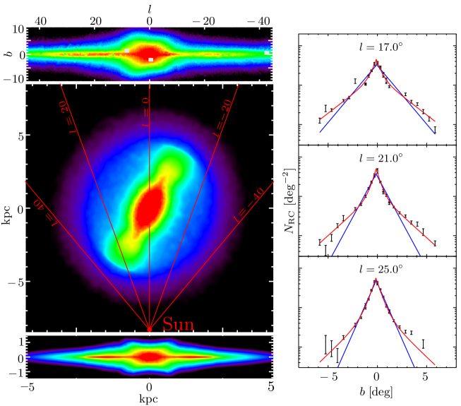
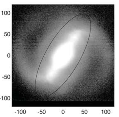
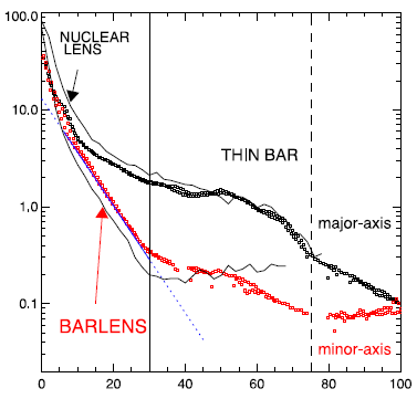
Comparing parametric models for the RCG magnitude distributions with the data, Wegg, Gerhard & Portail (2015) find a total bar (half) length of . Projections of their best model for the combined bulge and long bar are shown in Figure 9. The top panel illustrates the asymmetries seen by observers at the Sun, due to the bar shape and geometry. The side-on view in Fig. 9 clearly shows the Milky Way’s central box/peanut bulge and the decrease of the scale-height in the long-bar region. In the central face-on view, the projected b/p-bulge resembles the bar-lens structures described by Laurikainen et al. (2011), which are considered to be the more face-on counterparts of b/p-bulges (Laurikainen et al., 2014); see the image of NGC 4314 in Figure 10.
Long bar \entry, long bar angle \entry, bar half-length \entry, thin bar scale-height \entry, superthin bar scale-height \entry, stellar mass of thin bar \entry, stellar mass of superthin bar
In the same analysis, Wegg, Gerhard & Portail (2015) find evidence for two vertical scale-heights in the long bar, also illustrated in Fig. 9. The thin bar component has and its density decreases outwards roughly exponentially; it is reminiscent of the old thin disk near the Sun. The second superthin bar component has and its density increases outwards towards the bar end where it dominates the RCG counts. The short scale-height is similar to the 60- superthin disk found in the edge-on spiral galaxy NGC 891 (Schechtman-Rook & Bershady, 2013). Stars in this component have an estimated vertical velocity dispersion of and should be younger than the thin component. However, to have formed RCG they must have ages at least but star-forming galaxies have a strong bias towards ages around (Salaris & Girardi, 2002). Such a younger bar component could arise from star formation towards the bar end or from disk stars captured by the bar.
The dynamical mass of the long bar component has not yet been determined. The stellar mass was estimated by Wegg, Gerhard & Portail (2015) from the RCG density using isochrones and a Kroupa IMF. This resulted in a total non-axisymmetric mass for the thin bar component of , assuming a 10 Gyr old, -enhanced population, and for the superthin component, assuming a constant past star formation rate. Owing to its half-length and its total mass , the long bar may have quite some impact on the dynamics of the Galactic disk inside the solar circle, particularly on the gas flow and the spiral arms, but perhaps also on surface density and scale-length measurements in the disk (see Fig. 10). In Section 4.4 below, we summarize constraints on the bar’s corotation radius, which must be larger than .
4.4 Pattern speed
The pattern speed of the b/p bulge and bar, or equivalently its corotation radius , has great importance for the dynamics of the bar and surrounding disk. Despite a number of different attacks on measuring its value is currently not accurately known. An upper limit comes from determining the length of the bar and assuming that, like in external galaxies the Galactic bar is a fast bar, i.e., (Aguerri, Debattista & Corsini, 2003; Aguerri et al., 2015). Here the lower limit is based on the fact that theoretically, bars cannot extend beyond their corotation radius because the main -orbit family supporting the bar becomes unstable (Contopoulos, 1980; Athanassoula, 1992). The length of the long bar from starcounts is and the length of the thin bar component alone is (Wegg, Gerhard & Portail, 2015); thus a strong lower limit is and a more likely range is kpc, or for (§6.4).
Early determinations appeared to give rather high values of . The most direct method applied a modified version of the Tremaine-Weinberg continuity argument to a complete sample of OH/IR stars in the inner Galaxy (Debattista, Gerhard & Sevenster, 2002), giving (sys) for but depending sensitively on the radial motion of the LSR.
More frequently, the pattern speed of the bar has been estimated from hydrodynamic simulations comparing the gas flow with observed Galactic CO and H -diagrams. These simulations are sensitive to the gravitational potential, and generally reproduce a number of characteristic features in the -plot, but none reproduces all observed features equally well. Consequently the derived pattern speeds depend somewhat on the gas features emphasized. Englmaier & Gerhard (1999) and Bissantz, Englmaier & Gerhard (2003) estimated ( kpc) matching the terminal velocity curve, spiral arm tangents and ridges in the -plot. Fux (1999) obtained ( kpc) from a comparison to various reference features in the CO -plot; Weiner & Sellwood (1999) obtained ( kpc) from matching the extreme H velocity contour; Rodriguez-Fernandez & Combes (2008) obtained and kpc matching to the Galactic spiral arm pattern. The most recent analysis based on a range of potential parameters is by Sormani, Binney & Magorrian (2015). They conclude that overall a pattern speed of corresponding to matches best the combined constraints from the terminal velocity envelope, the central velocity peaks, and the spiral arm traces in the -diagram (for ).
Stellar-dynamical models of the Galactic b/p bulge also depend on and give estimated ranges for its value. Shen et al. (2010) and Long et al. (2012) find for the same N-body model matched to the brava kinematic data. The recent models of Portail et al. (2015) fitted additionally to the RCG density from Wegg & Gerhard (2013) give values in the range , placing corotation in the range (for ). These values could depend somewhat on the still uncertain gravitational potential in the long bar region.
A final method is based on the interpretation of star streams observed in the distribution of stellar velocities in the solar neighborhood as due to resonant orbit families near the outer Lindblad resonance of the bar (Kalnajs, 1991; Dehnen, 2000). Dehnen (2000) estimates ( for . Minchev, Nordhaus & Quillen (2007) find (). Chakrabarty (2007) and others argue that spiral arm perturbations need to be included, finding and . The latest analysis of the Hercules stream by Antoja et al. (2014) gives , , and when rescaled to . This is the current most precise measurement but is model-dependent; it would place corotation just inside the thin long bar and clearly within the superthin bar. It is just compatible with all the uncertainties; alternatively it may suggest that the Hercules stream has a different origin than the outer Lindblad resonance.
Considering all these determinations and the systematic uncertainties, we finally adopt a range of , or for our best estimated . More accurate dynamical modelling of a wider set of stellar-kinematical data, in particular from gaia, is expected to narrow down this rather wide range in the coming years (Hunt & Kawata, 2014).
Bar pattern speed \entry Bar corotation radius
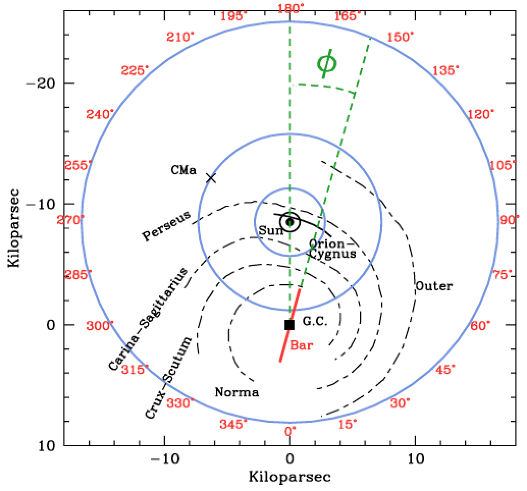
5 STELLAR DISK
Our vantage point from within the Galaxy allows us to obtain vast amounts of unique information about galactic processes but this detail comes at a price. The Solar System falls between two spiral arms (Fig. 11) at a small vertical distance from the Galactic Plane (§3.3). The thinness of the disk gives a fairly unobstructed view of the stellar halo and the outer bulge. But deprojecting the extended disk remains fraught with difficulty because of source confusion and interstellar extinction. Our off-centred position at the Solar Radius is a distinct advantage except that it complicates any attempt to learn about large-scale, non-axisymmetries across the Galaxy. We now have a better understanding of the structure of the inner Galaxy (§4) but the outer disk remains largely mysterious (see §5.5 below).
Over the past decade, we have learnt much about the Galactic stellar disk, but few parameters are known with any precision. The local surface density and the vertical density profile of the summed disk component (gas, stars, background dark matter) are known to high certainty (§ 5.4.1). But while photometric scalelengths are well established in external galaxies (Lange et al., 2015), the radial scalelengths and vertical scaleheights of the Galactic thin and thick disks are uncertain. Unlike for the inner Galactic bar/bulge region (§4), we are not able to present a fully consistent picture for the disk at this time, although the key parameters are discussed and values recommended. Major reviews of the stellar disk include Freeman & Bland-Hawthorn (2002); Ivezić, Beers & Jurić (2012); Rix & Bovy (2013); the gaseous disk is discussed at length by Kalberla & Dedes (2008).
One of the most interesting developments is the recognition of a Galactic ‘thick’ disk that is distinct from the dominant thin disk through its unique chemistry (e.g. Bensby, 2014; Masseron & Gilmore, 2015; Hawkins et al., 2015), in addition to its older age and higher elevation. Originally recognized by Gilmore & Reid (1983), such disks appear to be ubiquitous in the local universe (Yoachim & Dalcanton, 2006). In external galaxies, deep stellar photometry reveals that the thick and thin disks have approximately equal scalelengths (e.g. Comerón et al., 2012). Whether these old red disks have a distinct formation history or have continuous properties with the old thin disk is unclear. Several authors have presented models where the Galactic thick disk arises from a combination of stellar migration and/or flaring of the old disk stars, such that its history is tied to the formation of the thin disk even though its mean metallicity may be different (e.g. Schönrich & Binney, 2009; Loebman et al., 2011; Minchev et al., 2015). In view of the distinct chemical signature of the thick disk, it is worthwhile to quantify its properties separately from the thin disk regardless of its origins.
5.1 Stellar photometry
Early studies of the Galaxy fitted simple models to the projected star counts in a given optical or infrared band (e.g. Bahcall & Soneira, 1980). Without distance information, these authors found that a variety of models fit the data (including many combinations of two exponential functions) due to degeneracies between structural parameters. Historically, fits to star counts with vertical distance have used a variety of functions but, today, the exponential function is widely used to match both disk photometry (Patterson, 1940) and the peaked star counts close to the plane (Wainscoat, Freeman & Hyland, 1989).
By the end of the decade, we can expect accurate distances for millions of stars from the ESA gaia survey. But for now, we are dependent on photometric parallaxes for determining stellar distances which have a long history in their application to Milky Way structure (Gilmore & Reid, 1983; Kuijken & Gilmore, 1989; Chen et al., 2001). The term ‘parallax’ echoes the use of nearby bright stars with established trigonometric parallaxes to calibrate the absolute magnitude-distance relation (e.g. Eggen, 1951). (The term ‘spectroscopic parallax’ refers to the spectral classification used to determine the absolute magnitude, rather than photometric colours.)
5.1.1 Scaleheights
All photometric studies find an exponential scaleheight pc for the dominant old thin disk at the Sun’s location. The low extreme comes from multiband optical studies (e.g. Ojha, 2001) which include stellar populations with a wide range of (especially younger) ages. These surveys suffer from various biases that tend to suppress the scaleheight (see below). The upper extreme is from early M dwarf studies where confusion with halo M giants can lead to overestimates of the scaleheight (Reid, 1993; Gould, Bahcall & Flynn, 1996). M dwarfs, which account for roughly half of all stars in the solar neighbourhood (§ 5.4.2), trace the underlying total stellar mass. The much larger M star survey by Jurić et al. (2008), discussed below, finds pc (to within 20%) after various biasses are accounted for. This mid-range value is largely unchanged since Schmidt’s early determination (Schmidt, 1963).
An improvement is to use two or more well calibrated optical bands to compare the magnitude counts in different colour bins. This led to Gilmore & Reid’s identification of the thick disk after constructing the and luminosity functions for stars at or above the main sequence turn-off (MSTO) at different distances from the plane, and by ruling out biases due to interstellar extinction or metallicity gradients perpendicular to the disk. This classic study observed 12500 stars towards the South Galactic Pole (SGP) brighter than and provided the first reliable stellar densities vertical to the Galactic Plane their density profile continues to compare well with modern derivations (§ 5.4.1). They estimated pc in line with modern estimates, and pc, somewhat higher than what is believed today.
After 2000, the quality and angular extent of photometric data from wide-field CCDs improved dramatically (e.g. Finlator et al., 2000). The internal accuracies of the multiband data led to improved estimates of photometric parallax and metallicity (robust in the range -2 [Fe/H] 0) in wide-field surveys (see Ivezić, Beers & Jurić, 2012). Notably, Siegel et al. (2002) observed select Kapteyn fields to derive photometric distances for stars. They stressed the need to correct for unresolved multiplicities (of order 50%), otherwise stellar distances (and therefore scaleheights) are underestimated. The lower scaleheight estimates in the past are likely to have been underestimated for this reason. Even for old stars, there is some scaleheight variation among dwarfs: 280300 pc for early-type dwarfs () rising to 350 pc for late-type dwarfs (). When averaging over old dwarfs, before and after the correction, they obtain pc and pc respectively; for the thick disk, they find pc and pc respectively. (These are derived from exponential models; sech2 fits lead to 10% smaller values after correction for the factor of two difference in scaleheight between the exponential and sech2 functions.)
For our subsequent disk analysis, we focus on the sdss northern sky survey with its excellent photometric quality (0.02 mag). With photometric data for 48 millions stars over 6500 deg2, this is the largest to date with precise colourmagnitude vs. metallicity relations made possible using cluster calibrations across the sky (Finlator et al., 2000; Chen et al., 2001). This survey gave rise to three major studies based on photometric parallax (Jurić et al., 2008), photometric metallicities (Ivezić et al., 2008) and kinematics (Bond et al., 2010) discussed in the next two sections.
Juric et al (2008) exploit the faint magnitude limit ( mag) of the sdss survey and target two groups of M dwarfs: a late M group with and an early M/late K group with . The late M group is favoured because it is less sensitive to the halo population and to local substructure. At the Solar circle, their formal model fits for both disk components are pc and pc before correction for multiplicity, and closer to pc and pc after correction, both with 20% uncertainty. These constitute the most reliable values to date because of the sdss coverage in Galactic longitude and improved photometric distances over the required physical scales. While the sdss and 2mass surveys are widely used in star count analyses, neither survey is ideal for determining the properties of the thick and thin disks simultaneously. Rather than cross-matching sources common to both catalogues (e.g. Finlator et al., 2000), future studies will need to combine both surveys in order to provide better input catalogues (Robin et al., 2014).
While the thick disk was originally identified through stellar photometry, decompositions based on star counts are subject to degeneracies (§ 5.1.3). We include a limited discussion of the photometric estimates because of the historical context and because the thin disk values are broadly correct. But we stress that the thick and thin disk components are better separated through their distinct stellar chemistry. Numerous studies (§ 5.2) exploit either stellar abundances based on multiband photometry (large samples, large measurement errors) or spectroscopy (smaller samples, smaller errors).
5.1.2 Scalelengths
While vertical scaleheights are well determined at optical and IR wavebands due to the low extinction towards the poles, this is not true of disk radial scalelengths. We have analysed 130 refereed papers on disk parameters, with scalelengths ranging from 1.8 to 6.0 kpc. In order to combat the effects of extinction, for observations that preceded the sdss survey, the infrared point source measurements are the most reliable because they tell a consistent story. This is particularly true for studies that target a broad extent in Galactic longitude and observe in the anti-centre direction to ensure they are less influenced by the presence of the central bar or by substructure. These include the space shuttle experiment (Kent, Dame & Fazio, 1991), denis (Ruphy et al., 1996) in the anti-centre direction, cobe/FIRAS (Freudenreich, 1998; Drimmel & Spergel, 2001), 2mass (López-Corredoira et al., 2002; Cabrera-Lavers, Garzón & Hammersley, 2005; Reylé et al., 2009), and glimpse (Benjamin et al., 2005). A statistical analysis of the main papers (15 in all) on this topic leads to kpc which includes the highest value ( kpc) from the glimpse mid-infrared survey. Our estimate drops to kpc if we exclude the glimpse study.
We have already stressed the importance of M stars. Jurić et al. (2008) determine kpc (20% uncertainty) for the thin disk. Gould, Bahcall & Flynn (1996) and Zheng et al. (2001) used the Hubble Space Telescope to measure a scalelength of kpc and kpc respectively. All of these values are consistent with the IR measurements. A short scalelength finds strong support from dynamical studies of the stellar kinematics in §5.4. From a study of mono-abundance populations (MAP), Bovy et al. (2012b) conclude that different populations give a scalelength that is smoothly changing from 2 kpc in the inner disk (older populations) to 3 kpc at kpc (younger populations), or maybe even longer. However, the disk is dominated by old populations: a characteristic scale is meaningful when one considers the mass density profile of the disk. The IR photometric estimate of radial scalelength is probably the most useful at the present time, although we recognize that an exponential decline in the mass distribution is a crude approximation (Fig. 10). The thick disk scalelength is discussed in the next section.
For the past thirty years, some have argued for a longer disk scalelength when comparing the Galaxy, with its high mass and luminosity, to external galaxies (q.v. van der Kruit & Freeman, 2011). The gama survey (Driver et al., 2011) includes the largest bulge/disk decomposition survey to date using the viking K-band imaging survey of 4300 disk galaxies (Lange et al., 2015). This volume-limited survey has a high level of completeness to a redshift limit of (). Here only a few percent of galaxy disks exceed the Milky Way’s disk mass, and their IR photometric scalelengths have a large spread ( kpc). The Galaxy’s high luminosity and small scalelength may not be so unusual.
Disk substructure. We highlight one spectacular result from the sdss survey. The team was able to extract tomographic slices through the Galaxy vertical to the plane (e.g. Fig. 12). Fig. 12 illustrates a problem with Galaxy model fits and goes some way to explaining the lack of convergence in disk parameters over three decades. Jurić et al. (2008) explicitly highlight important substructure across the Galaxy including the ‘Virgo overdensity’ and the ‘Monoceros ring’ (Newberg et al., 2002). Substructure is so prevalent that it is not possible to fit a smooth double exponential disk model in and to either the thick or thin disk without taking this component into account. This problem is well known for disk-halo fitting because the Sgr stream dominates so much of the halo.
5.1.3 Thick disk normalization
Several studies have tried to determine the local density normalization () of the thick disk compared to the thin disk with estimates ranging from 1% to 12% (e.g. Gilmore & Reid, 1983; Siegel et al., 2002; Jurić et al., 2008). The large uncertainty in is largely due to its degeneracy with the derived scalelengths for both components (Siegel et al., 2002; Arnadottir et al., 2009): higher estimates of are associated with lower estimates of , and vice versa. To aid comparison with most published results, we prefer this form for rather than normalization to the total disk mass (e.g. Piffl et al., 2014a). We have analysed all results from photometric surveys (25 in all) since the discovery paper and arrive at .
A detailed analysis of the degeneracy between disk parameters is given by Chen et al. (2001) for late-type dwarfs chosen from the sdss survey where the data are separated into two hemispheres. Our value of is in line with their likelihood analysis (see their Fig. 9) for a thick disk scale height of kpc. It is also broadly consistent with dynamical fitting to the Solar cylinder (e.g. ; Just & Jahreiss, 2010).
The error is smaller when we compare the surface density of the thick and thin disks, i.e. . Here we find . Our analysis excludes all papers that do not fit simultaneously for the thin and thick disk. At this point, no separation is made on the basis of detailed stellar abundance information. A high thick disk local density () is also found when spectroscopic abundances are used to define the high [/Fe] population (Bovy et al., 2015) but this depends on how the abundance cut is made. A low value for is in conflict with Jurić et al. (2008) who determine the thick disk to be more massive () at the Solar circle (cf. Fuhrmann, 2008). Recent claims of a more massive thick disk may arise from the survey selection extending into the low [/Fe] population (e.g. Snaith et al., 2014) or from the use of a tiny survey volume (e.g. Fuhrmann, 2008).
pc, thin disk vertical scalelength at \entry pc, thick disk vertical scalelength at \entry, thick / thin disk local density ratio at \entry, thick / thin disk surface density ratio at \entry kpc, thin disk radial scalelength \entry, thin disk stellar mass
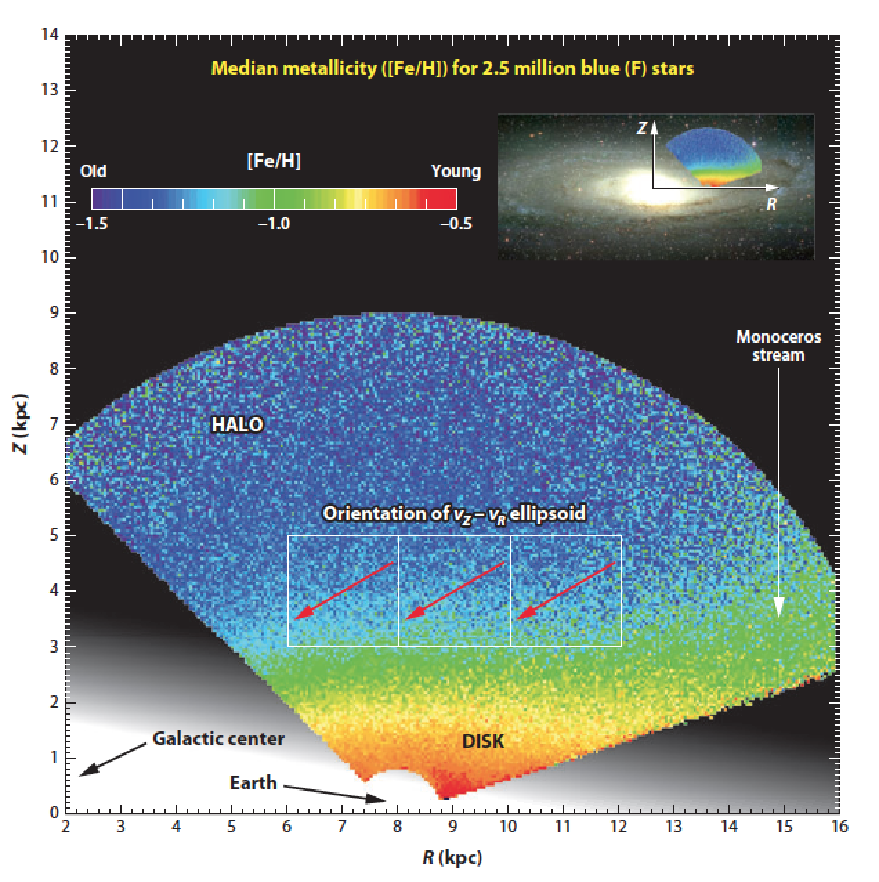
5.2 Stellar chemistry
5.2.1 Photometric metallicity
Ivezić et al. (2008) examined the vertical distribution in photometric metallicity of 2 million sdss stars calibrated with segue spectra of 60,000 F, G dwarfs (). An additional refinement was to combine the Palomar Optical Sky Survey (poss) and the sdss data to derive proper motions (e.g. Munn et al., 2004). Here the tangential velocity accuracy for stars brighter than is comparable to the radial velocity accuracy of the sdss spectroscopic survey (15 km s-1 for a star at 1 kpc; 100 km s-1 at 7 kpc). The aim was to look for the thin disk-thick disk transition at 1 kpc, and the thick disk-halo transition at 2.5 kpc, in metallicity and velocity. The sdss team confirm earlier trends in declining metallicity and increasing lag at larger elevations (Fig. 12), and find evidence for thick disk stars extending to kpc. They could only discern a gradual transition in photometric metallicity and kinematics across the thin disk-thick disk divide, in conflict with the traditional two-component fit (cf. Bond et al., 2010). While no kinematic modelling was conducted at this stage (see § 5.3), the sdss team find the data are more consistent with a gradual continuum from a thin young disk to an extended older disk. A better understanding of the thick disk vs. thin disk separation had to wait for spectroscopic surveys (§ 5.2) providing both improved elemental abundances and 3D space velocities (Steinmetz et al., 2006; Allende Prieto et al., 2008).
5.2.2 Spectroscopic metallicity
In the past, some researchers have questioned the existence of a thick disk with discrete properties chemistry, age, kinematics beyond the obvious characteristic of physical extent (e.g. Norris & Ryan, 1991). This is a fundamental question because it hinges on the formation and evolution of the major baryonic component of our Galaxy. In Fig. 13, the stars of the thick disk are mostly older than the thin disk and have a distinct chemistry (Bensby, Feltzing & Lundström, 2003; Schuster et al., 2006; Haywood, 2006; Bensby, 2014). It is recognized today that [/Fe] is enhanced for the thick disk compared to the thin disk over a wide range in [Fe/H], an effect that is easily seen in sufficiently high-resolution () spectroscopic data (Fuhrmann, 1998; Prochaska et al., 2000; Gratton et al., 2000; Reddy et al., 2003; Soubiran, Bienaymé & Siebert, 2003; Reddy, Lambert & Allende Prieto, 2006) even possibly at [Fe/H] 0 (Haywood et al., 2015; Hayden et al., 2015; Kordopatis et al., 2015). Recent studies show that the earlier counter claims likely suffered from underestimating measurement errors (e.g. Nidever et al., 2014) or incorrectly assumed that errors between measurements are uncorrelated (e.g. Schönrich, Asplund & Casagrande, 2014).
The kinematic criteria often used to separate the disks inevitably lead to small stellar samples compared to photometric surveys. The Bensby studies exploit the Geneva-Copenhagen survey of 16000 nearby dwarfs with full 3D space velocities, and ages and metallicities from Strömgren photometry (Nordström et al., 2004). But a clean local separation is hampered in part by extensive kinematic substructure over the local volume: the Hercules stream, for example, comprises both thick and thin disk stars (Bensby et al., 2007). But even without kinematic separation, the chemical signature of two distinct populations is evident (Adibekyan et al., 2012; Haywood et al., 2015).
A new signature has emerged from the apogee survey that may help to separate the disks further. Masseron & Gilmore (2015) show that C/N is enhanced in the thick disk compared to the thin disk, presumably due to the effects of dredge-up observed in old turn-off dwarfs and giants. The associated age (and mass) for the oldest stars is broadly consistent with Fig. 13. At the present time, it is not possible to separate the thick disk from the oldest thin disk stars through age-dating, assuming such a distinction even exists. The detailed chemistry of the thick disk may provide a better discriminator than the use of phase space (x,v) and be the defining characteristic of this component. Kinematic criteria will always lead to some overlap. Hawkins et al. (2015) emphasize that a more expanded chemical () space may be called for to ensure that the thick disk can be separated from both the thin disk and the lower halo, i.e. ([/Fe], [C+N/Fe], [Al/Fe], [Mg/Mn]). A high quality ‘chemical tag’ defined in this way requires both optical and infrared data at high spectroscopic resolution.
The use of chemistry to define thick disk stars now gives a different perspective on defining the relative density and scales of the two disks. Bensby et al. (2010) found that the bimodal [/Fe] distribution continues inside of the Solar Circle, in contrast to the outer disk where the enhanced [/Fe] population is not detected, which led Bensby et al. (2011) to infer a shorter scalelength for the thick disk. By dividing segue dwarfs spectroscopically into MAPs, Bovy et al. (2012b) note the transition between a short scalelength, “high [/Fe], low [Fe/H] population,” with a scaleheight up to 1000 pc, and a longer scalelength, “low [/Fe], high [Fe/H]” population, with a scaleheight below 400 pc. But the more extensive apogee survey of 70,000 red giants reveals that the picture is more complicated (Bovy et al., 2015; Hayden et al., 2015). Looking outwards, both tracks are evident, except the high [/Fe] sequence disappears beyond 11 kpc while the low sequence is seen to at least 15 kpc.
Towards the inner disk, the high [/Fe] track dominates over the low [/Fe] sequence even though an increasing fraction of stars pile up towards higher metallicity due to the thin disk abundance gradient. Over the innermost disk, the thick disk and bulge are more difficult to disentangle because they share kinematic and abundance characteristics, as observed in red giants (Alves-Brito et al., 2010; Ryde et al., 2010; Hill et al., 2011; Gonzalez et al., 2011b) and microlensed dwarf stars (Bensby et al., 2009, 2013).
In summary, estimates for the thick disk scalelength range from 1.8 to 4.9 kpc (12 papers) (e.g. Cheng et al., 2012; Larsen & Humphreys, 2003) but few of these make a distinction based on chemistry. There exists now some convergence on from surveys over very different volumes and sample sizes. Bensby et al. (2011) estimate an exponential scalelength of 2 kpc (10% accuracy), in good agreement with the high-[/Fe] MAPs from segue (Bovy et al., 2012b), although Cheng et al. (2012) measure kpc using 7000 MSTO dwarfs from the same survey, albeit with larger errors. More recently, Bovy et al. (2015) find kpc for high-[/Fe] MAPs using apogee red clump giants. Overall, we conclude that kpc where the thick disk is defined in terms of the high-[/Fe] population. When extrapolated to the Galactic Centre, the ratios and are 2.6 times higher than the local values. Thus, taking into account the shorter scale length of the thick disk, we estimate , or roughly one fifth of the thin disk mass.
kpc, thick disk radial scalelength \entry, thick disk stellar mass
5.3 Stellar kinematics
The large photometric surveys, with their photometric distance estimates, provide us with initial estimates of the structural parameters for each of the major Galactic components. Over a decade ago, the community recognized that progress would require kinematic information for many stars over large swaths of the sky. Since that time, there has been extensive investment in wide-field stellar kinematic surveys, some of which are still in progress: gcs (Nordström et al., 2004); segue (Yanny et al., 2009); rave (Steinmetz et al., 2006); apogee (Allende Prieto et al., 2008); legue (Deng et al., 2012); ges (Gilmore et al., 2012); and galah (De Silva et al., 2015). These surveys look at different parts of the sky and go to different depths. Some have been rendered dynamically as 3D visualizations at the following website: https://www.rave-survey.org/project/gallery/movies. The gcs survey covers the full sky but is confined to the Solar Neighbourhood; the segue, rave and apogee surveys penetrate deeper into the Galaxy than earlier stellar surveys. By far the largest of the new surveys, the ESA gaia mission will obtain both spectra and astrometric information for up to 150 million stars (de Bruijne et al., 2015). By the end of the decade, we can expect to have radial velocities and stellar parameters for millions of stars, for dwarfs out to 1 kpc, and for giants out to the halo.
Here we review the main insights to emerge from these surveys. We make a distinction between dynamical models of the Galaxy (e.g. Rix & Bovy, 2013, §6) and models that fit to the separate Galactic components without dynamical consistency (e.g. Catena & Ullio, 2010), which we refer to as kinematic models. In a kinematic model, one specifies the stellar motions independently at each spatial location, and the gravitational field in which the stars move plays no role. In a dynamical model, the spatial density distribution of stars and their kinematics are self-consistently linked by the potential, under the assumption that the system is in steady state.
When fitting a model, there are important considerations. First, all surveys are defined by their selection function (e.g. magnitude, velocity, coordinates) and any biasses must be accomodated by the analysis. Secondly, it is important to make a stab at including a plausible star formation history into the analysis (e.g. Schönrich & Binney, 2009). Making more stars in the past places more old stars at higher galactic latitudes today, and therefore higher kinematic dispersion through the age-velocity dispersion relation (e.g. Aumer & Binney, 2009). But this adds to the complexity because (a) we are introducing new variables into an already crowded field; and (b) degeneracy exists between different parameters, e.g. the star formation rate and the slope of the initial mass function (Haywood, Robin & Crézé, 1997).
An increasingly popular approach to fitting is to use Bayesian optimization over a broad set of free parameters (e.g. Catena & Ullio, 2010). As a worked example, in Appendix A, we summarize the framework for fitting up to 20 disk parameters this code is freely available at http://sourceforge.net/p/galaxia/wiki/Home/. The approach is theoretically simple and allows for useful constraints on local kinematic properties. The framework incorporates a constant star formation rate and a 3D Galactic dust model. Uniquely, it is designed to correct for an arbitrary survey selection function and can be used to fit data to analytic functions or numerical simulations (Sharma et al., 2011).
Sharma et al. (2014) apply the method in Appendix A to the rave and gcs surveys by assuming the structural form of the disk and then attempting to fit for from the surveys. They use only sky position and velocity for each star as these are the most accurate measurables. No distance information is supplied other than what is implicit in the model fitting. They fit both the Gaussian DF and the dynamically-motivated Shu DF (Sharma & Bland-Hawthorn, 2013); the latter performs better because it allows for asymmetric velocity distributions (relative to the Sun) due to non-circular motions experienced by most stars.
Groups that use Bayesian optimization (Bovy & Tremaine, 2012; Sharma et al., 2014) typically fit for (i) the age-velocity dispersion relation (see below); (ii) the radial scalelengths (, ) of the velocity dispersion profile; (iii) the mean stellar motion with vertical height ; and (iv) the solar motion (). The rave team find that earlier estimates of the local standard of rest (LSR) are unreliable if they neglect the vertical dependence of the mean azimuthal motion for a given population. Ultimately, even after this correction, global kinematic measures like are expected to have systematic uncertainties because of the initial assumption on and the lack of dynamical consistency. We return to these measures in the next section.
5.3.1 Age-velocity dispersion relation (AVR)
It is well established that the velocity dispersion of a disk stellar population increases with age (Strömberg, 1925; Wielen, 1977). Disks heat because a cold thin disk occupies a small fraction of phase space, and fluctuations in the gravitational field cause stars to diffuse through phase space to regions of lower phase space density. These effects are very difficult to model reliably through numerical simulations. For the thin disk, the AVR is sometimes approximated as a power-law in cosmic time (e.g. Aumer & Binney, 2009) such that
| (1) |
where () are priors. The power-law indices () provide important information on disk heating parameters (Binney, 2013; Sellwood, 2013); a summary of estimates is given in Table 4. The widely used value of dates back to the cloud scattering model of Spitzer & Schwarzschild (1953). While useful, this form is not universally accepted (e.g. Freeman, 2001; Quillen & Garnett, 2001); it makes no allowance for the thick disk which must be treated separately. From existing data, it is very difficult to distinguish a continually rising AVR from one that steps or saturates at old ages (Aumer & Binney, 2009; Casagrande et al., 2011). Some groups attempt to fit for age-metallicity trends in the thin disk but such fits are less instructive at the present time (q.v. Freeman & Bland-Hawthorn, 2002), although ultimately this information will need to be accommodated in a successful model (Sanders & Binney, 2015).
| Reference | Survey | |||
|---|---|---|---|---|
| Nordstrom et al. (2004) | GCS | |||
| Seabroke & Gilmore (2007) | GCS | - | - | |
| Holmberg et al. (2007) | GCS | 0.38 | 0.38 | 0.54 |
| Holmberg et al. (2009) | Hipparcos, GCS | 0.39 | 0.40 | 0.53 |
| Aumer & Binney (2009) | Hipparcos, GCS | 0.31 | 0.43 | 0.45 |
| Just & Jahrei (2010) | Hipparcos | - | - | 0.38 |
| Sharma et al. (2014) | GCS | 0.200.02 | 0.270.02 | 0.360.02 |
| Sharma et al. (2014) | RAVE | 0.190.02 | - | 0.3-0.4 |
| Sanders & Binney (2015) | SEGUE | 0.33 | - | 0.4 |
5.3.2 Velocity dispersion profile
Pasetto et al. (2012) used the rave survey to learn about the variation of velocity dispersion in the plane. They used singular value decomposition to compute the moments of the velocity distribution. As expected, the thin disk stars follow near circular, co-rotational orbits with a low velocity dispersion (e.g. Edvardsson et al., 1993; Reddy et al., 2003). The velocity dispersion falls as a function of distance from the Galactic Centre, consistent with theoretical expectation (Cuddeford & Amendt, 1992).
In an exponential disk, the stellar dispersion declines radially with the disk surface density and scale height as . Sharma et al. (2014) combined equation 1 with an exponential factor in radius (cf. van der Kruit, 1986) in order to determine the radial scalelengths (, ) of the dispersion profile (e.g. Lewis & Freeman, 1989). For an isothermal disk, is expected to be roughly twice the disk density scalelength (Bottema, 1993). The rave study confirms that the dispersion profile declines with radius, yielding estimates of 14 kpc and 7.5 kpc. The thick disk value is in good agreement with a full dynamical analysis which we return to below. The thin disk is insufficiently constrained in the rave survey because the elevated sightlines in latitude do not extend far enough in radius and are susceptible to vertical dispersion gradients (cf. Piffl et al., 2014a; Sanders & Binney, 2015).
Bovy, Rix & Hogg (2012a) divided up the segue survey into MAPs and argued that these constituted quasi-isothermal populations. (We refer the reader to Sanders & Binney (2015) for a different perspective on how to treat chemical information in fitting Galactic models.) Bovy found no break in vertical dispersion between the old thin and thick disk and suggested that the thick disk is a continuation of the thin disk rather than a separate entity (cf. Schönrich & Binney, 2009). In contrast, kinematic and dynamic studies which include a star formation history and an age-velocity dispersion relation explicitly for the thin disk do tend to find a break in the vertical stellar dispersion (e.g. Table 5). Future studies that exploit improved stellar ages and chemistry will be needed to resolve this issue.
5.3.3 Solar motion and LSR
Delhaye (1965) determined the solar motion with respect to the Local Standard of Rest (LSR) defined in the reference frame of a circular orbit that passes through the Sun’s position today. Formally, for a coordinate system based at the Sun, where the unit vector points towards the Galactic Centre, in the direction of rotation, and is upwards from the disk, . Delhaye studied different spectral classes and luminosity groups, and arrived at km s-1 that is very respectable by modern standards.
The random stellar motions of a given population is a strong function of their mean age, colour, metallicity and scaleheight. Care must be taken to account for the asymmetric drift of stellar populations in taking the limit to the zero-dispersion LSR orbit. Using Strömberg’s relation, Dehnen & Binney (1998) measured () (10.0, 5.2, 7.2) km s-1 from the hipparcos survey, which for two ordinates are in excellent agreement with Delhaye’s early estimates. was later revised upwards close to the original value (Binney, 2010; Schönrich et al., 2010); the latter paper showed that Strömberg’s linear asymmetric drift relation is invalidated by the metallicity gradient in the disk. Our values for in the margin note are averaged over most estimates since Delhaye’s original estimate. We have removed extreme outliers and ignored early values from any researcher who revised these at a later stage using a similar method. Thus, the Sun is moving inwards towards the Galactic Centre, upwards toward the NGP and, given , away from the plane.
While () have converged on Delhaye’s original values within the errors (see the margin note), some uncertainty surrounds when considered across the apogee, rave and legue surveys (Bovy et al., 2012d; Sharma et al., 2014; Tian et al., 2015). One reason for this may arise from local kinematic substructure or any systematic streaming motion in the Sun’s vicinity (Dehnen, 2000; Antoja et al., 2014; Siebert et al., 2011; Williams et al., 2013). A local spiral arm density wave, for example, can impose kinematic fluctuations of order 10 km s-1 (Siebert et al., 2012). In addition, because the corotation radius of the Galactic bar may be as close as inward from the Sun (§4.4), systematic streaming velocities may exist in the local Galactic disk due to perturbations from the bar and adjacent spiral arms. These could cause deviations of the zero-dispersion LSR orbit from the average circular velocity at , defined as the angular rotation velocity of a ’fictitious’ circular orbit in the axisymmetrically averaged gravitational potential, the so-called rotational standard of rest (RSR, see Shuter, 1982; Bovy et al., 2012d). Analysing two mostly independent samples of stars from apogee, rave and gcs, Bovy et al. (2015) modelled the disk velocity field over - scales and found such effects, with an implied tangential LSR streaming velocity of relative to the RSR. On the other hand, Sharma et al. (2014) find little difference in between the local GCS survey and the rave data which extends to , and Reid et al. (2014) when fitting their maser velocities with a circular orbit velocity field find no evidence for a deviation of the globally fitted from the locally determined value. Globally determined values of (Bovy et al., 2012d; Reid et al., 2014) agree well within errors with the locally determined . Here we adopt because we cannot establish clear agreement on the magnitude of the streaming motion at the present time. Future studies are anticipated which compare the impending gaia data with models including the central bar and spiral density waves in view of understanding both the random and streaming motions in the disk.
km s-1, solar motion in \entry km s-1, solar motion in \entry km s-1, solar motion in \entry km s-1, solar vector motion \entry km s-1, LSR streaming motion
5.3.4 Vertex deviation
Binney et al. (2014) revisit the rave data but include distance estimates using Burnett et al. (2011). These were not employed by Sharma et al. (2014) because rave distances are susceptible to uncertainties in proper motions and stellar parameters, e.g. log-g (Zwitter et al., 2010; Anguiano et al., 2015). After excluding young stars, Binney finds that the velocity dispersion for a given stellar population increases as one moves vertically in from the plane (cf. Smith et al., 2009). Furthermore, at any location in , the velocity ellipsoid’s long axis (vertex deviation) points towards the Galactic Centre (see Fig. 12), indicating that the radial and vertical motions of stars are intimately coupled (cf. Siebert et al., 2008; Bond et al., 2010). This important result demonstrates that the stellar motions in and are entwined through the Galactic potential.
| Parameter | M11 | B12a | BR13b | P14 | SB15 | BP15 |
| Kinematic data | H | GCS | SEGUE | RAVE | SEGUE | RAVE |
| (kpc) | 8.3 | [8.0-8.4] | [8.0] | [8.3] | [8.0] | [8.3] |
| (km s-1) | 239 | [220-241] | 218 | [240] | [220] | [240] |
| () | 1.3 | - | - | 1.3 | - | 1.4 |
| ()c | 7.1 | - | 6.8 | 5.6 | - | 6.2 |
| (%)d | 4.9 | - | - | 4.3 | - | 4.2 |
| (kpc) | 3.0 | 2.7-3.1 | 2.2 | 2.7= | 2.3 | 3.7= |
| (kpc) | 3.3 | 2.1-3.6 | - | 2.7= | 3.5 | 3.7= |
| (kpc)e | - | 3.6-20 | - | 9.0= | 7.8= | 2= |
| (kpc) | - | - | - | 9.0= | 7.8= | 2= |
| (kpc) | - | - | - | 13 | 6.2= | 11.6 |
| (kpc) | - | - | - | 4.2 | 6.2= | 5.0 |
| (km s-1) | - | 40-42 | - | 34 | 48 | 35 |
| (km s-1) | - | 20-27 | - | 25 | 31 | 26 |
| (km s-1) | - | 25-28 | - | 51 | 51 | 53 |
| (km s-1) | - | 33-65 | - | 49 | 51 | 53 |
aThe thin and thick disks are treated separately for two distinct potentials and parameter sets (b, c). b has been rescaled to = 8.3 kpc for ease of comparison with other results. c includes the stellar disk, the bulge and the cold gas disk; the M11 total stellar mass has been corrected for a gas mass of in line with the other references, except that BP15 assumes a gas mass of . assumes a spherical halo () with leading to higher values; does not include the Galactic corona; thin disk dispersions are evaluated at 10 Gyr. is the ratio of to the total galaxy mass. e is a parameter that sets the scale of the outward radial decline in velocity dispersion within the disk. Note: All models (except M11) apply Bayesian fitting of action integrals. Key: […] indicates a prior; ‘’ indicates values locked in fitting for . References: M11 - McMillan (2011); B12 - Binney (2012); BR13 - Bovy & Rix (2013); P14 - Piffl et al (2014a); SB15 - Sanders & Binney (2015); BP15 - Binney & Piffl (2015).
5.4 Stellar dynamics
Kinematic models offer greater freedom than physics really allows. This can lead to systematic errors in parameter estimation which typically swamp the statistical errors in the optimization scheme. The way forward is to consider dynamical models such that the spatial density distribution of stars and their kinematics are linked by the gravitational potential , under the assumption that the system is in steady state. At present, dynamical models are used to estimate a subset of parameters explored by kinematic methods (see Table 5). While there has been good progress in recent years, with the first signs of dynamical self-consistency beginning to emerge, there is no fully consistent framework at the present time. We refer the reader to Rix & Bovy (2013, §6) for a useful summary of the dynamical methods on offer.
Early methods that operate locally or in annular bins (e.g. Bienayme, Robin & Creze, 1987; Just & Jahreiss, 2010) have given way to holistic treatments over one or more dynamical components of the Galaxy (e.g. Piffl et al., 2014a; Sanders & Binney, 2015). Dynamical models assume an equilibrium figure such that the phase space density of stars links only to the phase space coordinates through the constants of motion (Jean’s theorem).
Binney (2010, 2012) has argued that action integrals () are ideal for building dynamical models because they are adiabatic invariants. The most convenient action integrals are (i) , the approximate symmetry axis of the Galaxy’s angular momentum, (ii) , to describe the action of a star perpendicular to the plane, and (iii) , to describe the radial action of the star. The DF at any point in the Galaxy has the form . is derived through an iterative process starting with an initial guess to get to the density integrated over the phase-space volume . Poisson’s equation is used to compute an updated and the process is repeated until convergence is achieved. The numerical procedures are non-trivial and computationally expensive, but entirely feasible for surveys involving thousands of stars (Binney & McMillan, 2011).
Of the few action integral studies of the disk to date, we highlight the work of Binney (2012) using gcs; Bovy & Rix (2013) and Sanders & Binney (2015) using segue; Piffl et al. (2014a) and Binney & Piffl (2015) using the rave survey. In Table 5, these studies attempt to arrive at unbiassed parameter estimates through fitting the data with a consistent dynamical model. Binney (2012) introduced important new ideas in model fitting, including the use of the quasi-isothermal DF to model the disk. But his focus on a very local sample led to the disk dispersions being underestimated due to the gcs bias towards younger stars. As we return to below, this work has been superseded by Piffl et al. (2014a) who determined the DF from the rave giants. The rave survey comprises roughly equal numbers of dwarfs and giants, most within about 2.5 kpc of the Sun, and is thus more representative of the extended disk (Sharma et al., 2011).
Bovy & Rix (2013) build on Binney (2012) using 16300 G dwarfs from the segue survey. They divide stars in the abundance plane into MAPs: the more metal-rich MAPs trace the inner disk whereas the metal-poor populations trace the disk beyond the Solar Circle. Their goal is to measure the Galactic disk’s mass profile by identifying a radius for each MAP where the modelling gives a tight (statistical) constraint on the local surface density. It is unclear whether (a) most MAPs can be treated as quasi-isothermal populations; and (b) the constraints at different radii from the MAPs are mutually consistent, i.e. free of systematic errors (e.g. Sanders & Binney, 2015). The disk scalelength is the most important unknown in disentangling the contributions from the disk and the dark halo to the mass distribution near the disk. In contrast to the photometric radial profile, without dynamical consistency, the mass-weighted radial profile cannot have been reliably measured in earlier kinematic studies.
Sanders & Binney (2015) revisit the segue analysis and instead treat the chemical (and phase) space as a continuous distribution. They introduce the idea of an ‘extended distribution function’ (EDF) in place of the DF where Z defines the chemical domain. While different abundance groups can have very diverse kinematics, they all necessarily reside within the same Galactic potential; the extra information in the EDF allows for a more accurate treatment of the selection function and associated errors across the survey. They determine that the thick disk vertical dispersion is a factor of two larger than the thin disk value ( 25 km s-1), in agreement with Sharma et al. (2014) and Piffl et al. (2014a). Unlike either of these studies, they obtain sensible numbers for both and for the first time, with a disk scalelength ( kpc) 35% smaller than the thick disk (Table 5), but in conflict with the apogee survey (Hayden et al., 2015). (While defines the scale of the outward decline of the stellar dispersion, it is not the exponential radial scalelength used in the kinematic studies because DFs are expressed in terms of integrals of motion, not radii.) Sanders & Binney state that their analysis is only preliminary because was kept fixed throughout. Arguably, this study comes closest to the ideal of chemodynamical self-consistency. In the margin note, we adopt the rave velocity dispersions (Piffl et al., 2014a) as these are consistent across studies and extend further into the lower latitudes of the disk. {marginnote} \entry, old thin disk radial velocity dispersion at \entry, old thin disk vertical velocity dispersion at \entry, thick disk radial velocity dispersion at \entry, thick disk vertical velocity dispersion at
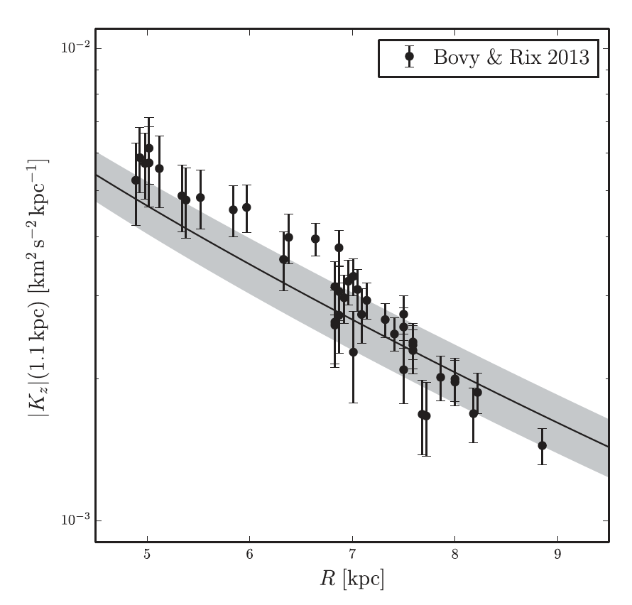
5.4.1 Vertical density and acceleration
Measurements of the local baryon and dark matter density have a long tradition in astronomy (Kapteyn, 1922). From a survey of K giants towards the SGP, (Kuijken & Gilmore, 1989) went further and attempted to derive the vertical density profile and the gravitational acceleration induced by the local disk that are related through Poisson’s equation . This is transformed into a surface density such that
| (2) |
evaluated over the column kpc or . As McKee, Parravano & Hollenbach (2015) point out, this must be done with care. The usual assumption that for a flat rotation curve at the midplane leads to an error because, in this instance, the rotation curve cannot be flat at a fixed height off the plane. In any event, this is a difficult measurement to get right because stellar surveys are strongly biassed towards more distant stars (cf. Zheng et al., 2001).
We can be confident that we do understand the local acceleration of the disk and the make-up of the local density (§ 5.4.2) over a vertical distance of kpc (Kuijken & Gilmore, 1989; Bovy & Tremaine, 2012). A dynamical fit to 200,000 giants in the rave survey (Piffl et al., 2014a) leads to a local determination of and its local gradient (Fig. 14) which are in generally good agreement with the segue dwarf analysis.
The vertical density profile determined by Gilmore & Reid for dwarf stars has survived the test of time. Modern surveys are either too shallow (e.g. 2mass) or too deep (e.g. segue) to properly represent the disk although good agreement is found with the sdss dwarf photometry (Jurić et al., 2008) after careful re-analysis (Piffl et al., 2014a). Binney et al. (2014) note that the kinematics of the cool dwarfs and giants in rave are consistent, such that dynamical model fits for giants or dwarfs can reasonably adopt Gilmore & Reid (1983) as a starting point, as has been done by most dynamical studies.
Given Gilmore & Reid (1983) or a similar density profile (e.g. Kuijken & Gilmore, 1989), the dynamical modelling attempts to find a self-consistent mass model-DF pair. This means that the mass distribution of the stellar disk implied by the DF in the potential is consistent with the mass distribution of the stellar disk assumed in the mass model. The action integral analysis of Piffl et al. (2014a) used 200,000 giants in the rave survey. In Fig. 14, they find remarkable dynamic self-consistency in the local disk as defined above. Moving away from the solar neighbourhood, they infer a declining vertical force with as expected, in good agreement with the Bovy & Rix (2013) analysis of segue dwarfs ( kpc). The latter study derived a mass-weighted scalelength of kpc, smaller than the kpc (without a quoted error) inferred by the rave analysis. is dynamical by nature and is blind to the separate contributions of the ISM and the thin/thick disks.
5.4.2 Local mass budget
In a new study, McKee, Parravano & Hollenbach (2015) revise the local baryon inventory of Flynn et al. (2006) in light of new observations. Inter alia, they update the present day stellar mass function, and the vertical distributions and extents of both gas and stars. They find the baryon surface density integrated to infinity is pc-2 comprising brown dwarfs (1.2 pc-2), white dwarfs (4.9 pc-2), ISM gas (13.7 pc-2), main sequence and giants (27.0 pc-2). Interestingly, that least understood of main sequence stars - the M dwarf - makes up more than half of all stars by mass locally. Over the column kpc, there is general agreement that the total surface density (baryons dark matter) is pc-2 (Kuijken & Gilmore, 1989; Catena & Ullio, 2010; McMillan, 2011; Bovy & Rix, 2013; Piffl et al., 2014a).
In terms of local density, the proportion of each mass constituent is very different due to the wide spread in scaleheights. McKee, Parravano & Hollenbach (2015) give the local mass density as pc-3 ( GeV cm-3) comprising stars ( pc-3), gas ( pc-3), baryons ( pc-3), and dark matter ( pc-3).
pc-2, total mass surface density kpc at \entry pc-3, local mass density at \entry GeV cm-3, local dark matter energy density at
5.5 Outer disk
The physical extent and detailed structure of the outer disk is highly uncertain. Over the years, different authors have claimed evidence for an “edge” in the stellar disk in the range kpc from both optical and infrared surveys (Habing, 1988; Robin, Creze & Mohan, 1992; Ruphy et al., 1996; Minniti et al., 2011). When looking at external galaxies, what appear to be edges can be inflexions in the stellar density, i.e. a break in the exponential density profile. Such “breaks” are common (Pohlen & Trujillo, 2006) but “continuously exponential” disks are also known and the stars can extend to the observed edge of the HI disk (Bland-Hawthorn et al., 2005; Irwin et al., 2005; Ellis & Bland-Hawthorn, 2007).
Many new observations confirm that the outer disk is very complicated. The outer disk warps slowly away from the Galactic Plane in both H (May et al., 1993) and stars (Carney & Seitzer, 1993). In addition to the warp, the outer disk flares in both stars and gas and possesses a fair degree of substructure. Moni Bidin, Carraro & Méndez (2012) review the contradicting claims for the flaring stellar disk, but the comprehensive study of Momany et al. (2006) puts the issue beyond doubt. Carraro (2015) reviews the evidence for flaring in the outer disk in both young (HII regions, open clusters) and old stellar populations (cepheids, pulsars). The earlier claims of a disk edge did not consider the effect of a warping, flaring disk such that there is no strong evidence for a truncation to date in either old or young populations (López-Corredoira et al., 2002; Sale et al., 2009; Carraro et al., 2010).
A complicating factor is the presence of the near-planar Monoceros Ring at kpc (radial width 2 kpc) which appears to corotate at roughly the speed of the outer disk (Newberg et al., 2002; Ibata et al., 2003). The nature of this stream is unknown (cf. Xu et al., 2015): unlike the Canis Major overdensity which may be related to the warp, the ring appears to have its own identity after correcting for the warp (Momany et al., 2006), and may even rotate slightly faster than the disk (Ivezić et al., 2008).
Before the optical studies, H observations by Burton (1988) and Diplas & Savage (1991) identified Galactic gas out to at least kpc (see also Hartmann & Burton, 1997). Molecular gas clouds are seen to kpc, some with ongoing star formation (Yasui et al., 2008; Kobayashi et al., 2008). Further evidence for recent star formation out to these distances is the presence of young stars and open clusters (Carraro et al., 2010; Magrini et al., 2015). Remarkably, Kalberla & Dedes (2008) have pushed the H frontier to kpc which is within range of the orbiting Magellanic Clouds. The stellar/gaseous warp may be highly transient, triggered by the passage of the MC or Sgr dwarfs, with bending waves that travel at 20 kpc Gyr-1 near the Solar Circle; and are the local surface density and angular velocity of the disk respectively.
6 Halo
In this section, we review the stellar, gaseous, and dark matter halos of the Galaxy, and finally put together a global rotation curve for the Milky Way. This analysis brings together many of the key themes of the review. The stellar and dark matter halos share the property that they are three-dimensional structures surrounding the disk and still grow by accreting matter. However, they do not necessarily share the same structural properties or formation histories. The gaseous halo is an important repository for a part of the Galaxy’s baryonic mass, and interacts with the environment through inflows and outflows.
All three components live in the same gravitational potential, which at intermediate radii () is shaped by the Galactic bulge, disk and dark halo, and at large () radii is completely dominated by the dark matter. One important goal of studying the halo and the satellites around the Milky Way is to map out the large-scale gravitational potential - this is a major science goal of the ongoing gaia mission.
6.1 Stellar halo
The Milky Way’s stellar halo, although containing just of the total stellar mass, is an important component for unravelling our Galaxy’s formation history. It was first identified as a population of old, high-velocity, metal poor stars near the Sun, similar to the stars in globular clusters. The halo stars showed large random motions, little if any rotation, and a spheroidal to spherical spatial distribution. Following the influential paper of Eggen, Lynden-Bell & Sandage (1962), the classical view of the halo developed, of a smooth envelope of ancient stars from the time when the Galaxy first collapsed. Subsequently, Searle & Zinn (1978) suggested that the halo is built up from independent infalling fragments, based on their observation that halo globular clusters showed a wide range of metal abundances independent of Galactocentric distance.
Modern data from large stellar surveys show that the stellar halo has a complex structure with multiple components and unrelaxed substructures, and continues to accrete matter in the form of smaller galaxies which are then tidally disrupted in the gravitational field (e.g., Ibata et al., 1997; Belokurov et al., 2006; Schlaufman et al., 2009). This confirms the predictions of hierarchical galaxy formation models. Because of the long dynamical timescales in the halo, tidal tails, shells, and other overdensities arising from accreted dwarf galaxies remain observable over Gyrs, thus constituting a fossil record of the Milky Way’s accretion history. Previous reviews on this subject can be found in Helmi (2008); De Lucia (2012); Belokurov et al. (2013).
Cosmological simulations reveal that the Galaxy should have accreted satellite galaxies which would mostly have been disrupted by the tidal field, causing the build-up of the stellar halo. Irregular density distributions are predicted in the outer halo due to shells and tidal streams, with a large variance between different galaxies of the same dark matter halo mass. In these models, the majority of the halo is often built at early times, ago, and most of the stellar halo stars come from the disruption of one or a few massive satellites accreted early-on. The outer halo is built more recently than the inner halo and the halo properties evolve, reflecting the history of accretion (Bullock & Johnston, 2005; Font et al., 2006; De Lucia & Helmi, 2008; Cooper et al., 2010; Pillepich et al., 2014).
Part of the inner halo may have formed in situ, i.e., within the main body of the Galaxy (Abadi, Navarro & Steinmetz, 2006). Recent simulations suggest that a fraction of stars formed in the early Galactic disk could have been ejected into the inner halo, and further in situ halo stars could have formed from gas stripped from infalling satellites (Font et al., 2011; McCarthy et al., 2012; Tissera et al., 2013; Pillepich, Madau & Mayer, 2015; Cooper et al., 2015), but the quantitative importance of these processes is not yet fully understood. Observationally, evidence for a dual halo has been put forward by Carollo et al. (2007); Beers et al. (2012), but see Schönrich, Asplund & Casagrande (2014).
In this section we review the structural parameters of the Milky Way’s stellar halo and put them in the context of these hierarchical models. Determination of the mass of the dark matter halo based on these data is discussed in §6.3.
6.1.1 Halo flattening and average density profile
The stellar density of the halo is important because it reflects the cumulative past accretion history of the Milky Way. It has been extensively studied using several tracers for which good distances can be determined, including RR Lyrae (typical distance accuracy , Vivas & Zinn, 2006), blue horizontal branch (BHB) stars (, Belokurov et al., 2013), red giants (RGB, , Xue et al., 2014), and near-main sequence turnoff stars (nMSTO, with multiple colors, Ivezić et al., 2008). RR Lyrae and BHB stars, which trace the old metal-poor populations, are rarer than RGB and nMSTO stars, but can reach to galactocentric radius. RGB trace all halo populations and currently reach to about , whereas nMSTO stars are abundant and best for the inner halo, i.e. .
A significant fraction of these halo tracer stars is found in large substructures (§6.1.2). Subtracting these leads to an estimate of a smooth halo component (e.g., Deason, Belokurov & Evans, 2011), which however may contain smaller, yet unresolved substructures (e.g., Sesar et al., 2013). The spatial distributions of the halo stars are typically fitted by spherical or axisymmetric density models with single (SPL) or double (DPL) power-law or Sersic radial profiles, and with one or two flattening parameters for the inner and outer halo; Table 6 shows recent results based on DPL models. The inner halo flattening is found across various studies based on data reaching down to (see also Bell et al., 2008; Jurić et al., 2008). The inner power-law slope is encompassed by . (The quoted formal fit errors are often quite small, but this could easily depend on the chosen parametric form, the data volume, and on remaining substructures in the data.) No evidence is found for an outward gradient in for the RR Lyrae and BHB samples, but Xue et al. (2015) with RGB and Pila-Díez et al. (2015) with nMSTO find an increase to by .
| Reference | Tracer | [kpc] | - | [kpc] | - | |
|---|---|---|---|---|---|---|
| Xue et al. 2015 | RGB | |||||
| Pila-Diez et al. 2015 | nMSTO | |||||
| Sesar et al. 2011 | nMSTO | |||||
| Deason et al. 2011 | BHB/S | |||||
| Faccioli et al. 2014 | RRL | fixed | ||||
| Sesar et al. 2013 | RRL | |||||
| Sesar et al. 2010 | RRL | fixed | ||||
| Watkins et al. 2009 | RRL | fixed |
Halo density parameters from recent studies of halo tracer stars with oblate double power-law models. Columns give reference, tracer used, covered Galactic radius range, inner power law slope, inner halo axis ratio, break radius, and outer power-law slope (in these models, the outer ). Watkins et al. (2009) and Sesar et al. (2010) considered spherical DPL models; the numbers given in these lines are from a reanalyis by Faccioli et al. (2014).
Halo density \entry Inner density slope \entry Outer density slope \entry Break radius \entry Inner halo flattening \entry Outer halo flattening
There is clear evidence that the stellar halo profile steepens with radius; see Table 6. In the context of DPL models based on data reaching , the break radius between the inner and outer components scatters in the range . For RRL and BHB, the outer power-law slope is in the range , and Deason et al. (2014) found an even steeper profile beyond . For RGB the slope is somewhat shallower, . The overall density profile is similar to an Einasto function (e.g., Xue et al., 2015), and qualitatively similar to density profiles predicted by halo formation models (Bullock & Johnston, 2005; Cooper et al., 2010). Deason et al. (2013) use simulations to show that a distinct density break may be related to the accumulation of stars at their apocenters, following relatively massive accretion events. Lowing et al. (2014) point out that the measured density parameters depend strongly on the surveyed sightlines and halo accretion history.
6.1.2 Stellar halo mass and substructure fraction
Estimating the stellar halo mass from these density distributions is non-trivial, requiring determination of the mass normalisation per halo tracer star from stellar population models and calibrations, as well as extrapolating beyond the survey volume through models. Bell et al. (2008) fitted DPL models to SDSS nMSTO stars and found a best-fit stellar halo mass within of . Deason, Belokurov & Evans (2011) gave an estimate for the ratio of BHB stars per luminosity of , using data for Galactic globular clusters. With a mass-to-light ratio for metal-poor Galactic globular clusters (Kimmig et al., 2015), the estimated stellar halo mass within becomes .
The Milky Way halo contains numerous substructures which contain a significant fraction of its stellar mass (see Belokurov et al., 2013, for a review). The four largest stellar structures are the Sagittarius Stream, the Galactic Anti-Center Stellar Structure, the Virgo Overdensity, and the Hercules-Aquila Cloud. Estimated masses for these structures are, respectively, based on the luminosity from Niederste-Ostholt et al. (2010) and from Kimmig et al. (2015); (Yanny et al., 2003; Belokurov et al., 2013), (Bonaca et al., 2012) (iv) based on Belokurov et al. (2007), alltogether summing to . A significant fraction of this substructure mass is within the volume traced by the sdss nMSTO stars. We therefore add of this mass to the result of Bell et al. (2008) to obtain a rough estimate for the total stellar halo mass . This is somewhat lower than the classical value based on Morrison (1993).
Halo mass \entry Substructure mass \entry Total stellar halo mass
Bell et al. (2008) also quantified the fraction of mass in substructures from the ratio of the rms deviation of the density of nMSTO stars to the total density given through a smooth halo model. They find , arguing that much of the halo was accreted from satellite galaxies. In their study of BHB stars, Deason, Belokurov & Evans (2011) found a lower with some increase for fainter stars (larger distances); on this basis they argue for a smooth halo with superposed additional substructures. Reasons for the discrepancy between both studies could be the less accurate nMSTO distances, leading to blurring of compact substructures, the lower resolution with the rarer BHB stars, or because the BHB stars trace an older, more mixed population of stars (Deason, Belokurov & Evans, 2011). Resolving this issue requires large samples of stars with accurate distances and velocities. The problem is that even a fully accreted halo will eventually mix to be smooth above a given scale, and that mixing times are shortest in the high-density inner regions.
6.1.3 Halo rotation, velocity dispersion and anisotropy
Bond et al. (2010) analyzed the largest sample so far of halo star velocities within from the Sun, including SDSS stars with three velocity components. They found (i) a mean rotation of halo stars (their Fig. 5) of for our adopted and (§6.4); (ii) a velocity ellipsoid whose principal axes align well with spherical coordinates; and (iii) corresponding halo velocity dispersions , with a total error in each component of . These values are in excellent agreement with results from Smith et al. (2009). Note that the close alignment of the halo velocity ellipsoids with spherical coordinates does not imply a spherical potential (see Evans et al., 2016).
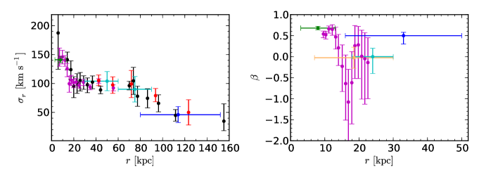
Fig. 15 shows the radial velocity dispersion profile in the outer halo based on several data sets. sharply decreases from the local to at , then remains approximately flat until , and finally decreases to about at . At the largest radii, where the stellar density profile is largely unknown (see Table 6), the very low values are consistent with a tidal truncation of an extrapolated steep power-law (Kafle et al., 2014).
Local halo kinematics \entry () Spherical velocity ellipsoid \entry Mean rotation
Tangential velocities can be estimated from the variation of LOS velocities across the sky and from proper motions. Fermani & Schönrich (2013) used BHB stars reaching to and with both kinds of methods find no rotation in either the inner or outer halo, and no trend with metallicity. Tangential velocity dispersions and the spherical anisotropy parameter were determined in the outer halo by several authors and are shown in Fig. 15. The radial anisotropy at small and large radii is consistent with predictions for accreted halos (Abadi, Navarro & Steinmetz, 2006). The tangential anisotropy at radii around was confirmed by King et al. (2015) but was suggested to be transient based on orbit simulations (Bird & Flynn, 2015), perhaps due to a yet unknown substructure in the halo.
6.2 Hot halo
The existence of a diffuse hot plasma (or corona) surrounding the Galactic disk has been widely discussed since Spitzer’s early observation that the ubiquitous HI clouds must be confined by an external medium (Spitzer, 1956). But it remains uncertain how much of the gas lies close to the Galactic plane, and how much of it extends into the halo (Bland-Hawthorn & Cohen 2003). Strong evidence for extended coronae have come from the first reliable detections of hot halos around nearby massive disk galaxies (e.g. Anderson & Bregman, 2011). The Galactic corona also explains the remarkable observation of gas depletion in all dwarfs within a radius of about 270 kpc, with the exception of the high-mass LMC and SMC dwarfs (Grcevich & Putman, 2009), which is well understood in terms of ram-pressure stripping by a hot medium (Nichols & Bland-Hawthorn, 2011; Gatto et al., 2013). Such an extended hot phase is supported by numerical simulations (Nuza et al., 2014) which focus on the properties and distribution of the multiphase gas in and around two simulated galaxies chosen as an M31-Galaxy analogue. They found the hot (K) gas has a uniform temperature profile around each of the simulated galaxies, and good agreement between the observed profile (Miller & Bregman, 2015) and the density profile of the simulated Galaxy.
| Reference | [kpc] | [cm-3] | [K] | [] | Method |
|---|---|---|---|---|---|
| BR00 | 1 | ram-pressure stripping | |||
| of gas in dwarf spheroidals | |||||
| S+02 | pressure equilibrium between | ||||
| HVCs (MS) and coronal gas | |||||
| S+03 | OVI absorption (100 LOS) | ||||
| BR07 | OVII absorption (25 LOS) | ||||
| uniform spherical halo | |||||
| AB10 | 3.5 | LMC pulsar dispersion measures | |||
| G+13 | ram-pressure stripping of gas | ||||
| in Carina and Sextans | |||||
| MB15 | OVII / OVIII emission (650 LOS) | ||||
| S+15 | ram-pressure stripping | ||||
| of the LMC disk |
Unless otherwise indicated, all coronal masses are integrated out to ; the gas density is quoted as a total particle density unless otherwise indicated. Notation: aAverage density out to the given distance; bDistance from the Galactic plane; cElectron density; dAssumed; eDistance from the Sun; fMass enclosed within 20 kpc; gMass enclosed within kpc. References: BR00 - Blitz & Robishaw (2000); S+02 - Stanimirović et al. (2002); S+03 - Sembach et al. (2003); BR07 - Bregman & Lloyd-Davies (2007); AB10 - Anderson & Bregman (2010); G+13 - Gatto et al. (2013); MB15 - Miller & Bregman (2015); S+15 - Salem et al. (2015).
We tabulate the most recent observations of the Galactic corona in Table 7. The best evidence for a hot corona comes from bright AGN sight lines with detections of O and O in absorption, and in high-resolution x-ray spectra (Paerels & Kahn, 2003) of a nearly ubiquitous soft x-ray background (SXRB) with energies (implying temperatures ), with some contribution of O and O in emission (Snowden et al., 1997; Henley & Shelton, 2012). The sensitivity of current x-ray spectroscopy limits O and O detections to a handful () of sight lines. There is an additional difficulty in disentangling the contribution of the Local Bubble, a supernova remnant in which the Solar System is embedded (Snowden et al., 1990), and the contribution from solar wind charge exchange processes, which produce soft x-ray emission throughout the Solar System (Cravens, Robertson & Snowden, 2001). Consequently, the detailed structure (density, temperature, entropy profile) of the Galactic corona, and hence its total mass, is uncertain.
The Galactic hot halo is likely to comprise two main components: one, exponentially decaying, high-metallicity () component with a scale height of a few kpc, which dominates the x-ray observations; and an extended (), more diffuse, low-metallicity halo (Yao & Wang, 2007). Purely exponential gas density profiles (i.e. not characterised by a single temperature) overpredict the coronal temperature and x-ray surface brightness by factors of a few (Fang, Bullock & Boylan-Kolchin, 2013).
Early attempts to model the corona using x-ray observations assumed (unphysically) that it was isothermal and at a constant density (Bregman & Lloyd-Davies, 2007; Gupta et al., 2012). The studies arrived at wildly different conclusions: the first study derived an electron density at ; the second found at (cf. Wang & Yao, 2012). Fang, Bullock & Boylan-Kolchin (2013) favoured a picture in which the corona is composed of adiabatic (isentropic) gas in hydrostatic equilibrium with the Galactic potential, in conflict with evidence that the Galactic halo is far from having a constant entropy profile (Miller & Bregman, 2015; Crain et al., 2010). It is now well established that the halo temperature as inferred from x-ray observations is fairly uniform across the sky and with little scatter around (Henley et al., 2010) although this does not demand that the halo is strictly isothermal.
A new all-sky catalog of O and O emission lines (Henley & Shelton, 2012) has been studied by Miller & Bregman (2013) and Miller & Bregman (2015). They used this catalogue in combination with x-ray measurements to determine that the halo density is of order to at . They determine a coronal gas mass of within . These results rely on key assumptions: (i) the density profile of the hot gas is well described by a spherically symmetric -model of the form , consistent with a truncated King model for the halo potential; (ii) the halo is isothermal with a temperature ; (iii) the gas is in collisional ionisation equilibrium. Miller & Bregman’s model can be justified if the dark matter halo of the Galaxy is well described by a spherically symmetric isothermal sphere with a core radius , and if the gas is quasi-isothermal and in approximate hydrostatic equilibrium with the potential.
Tepper-Garcia, Bland-Hawthorn & Sutherland (2015) bring all of this work together and search for a physically plausible corona that is consistent with the observed stellar halo dynamics and with the UV/x-ray measurements (Table 7). They normalise the dark matter halo to the density profile and total mass inferred from the kinematics of halo stars (Kafle et al., 2012). If the dark matter halo is isothermal, the core radius is somewhat larger than inferred from Miller & Bregman’s model, i.e. . The halo velocity dispersion implies a gas temperature of , leading to a density profile which is in broad agreement with Miller & Bregman (2015) and Nuza et al. (2014) with about the same total gas mass. The most likely baryonic mass range for the Galactic corona is .
The Galaxy’s baryonic mass fraction. The dynamical analyses presented in § 5.4 are relatively consistent in their estimates of the baryonic mass fraction of the Galaxy (stars cold gas), i.e. (Table 5). We now add the likely contribution from the hot corona within to arrive at a total baryonic mass, . This leads to a baryonic mass fraction out to of / which falls well short of the Universal value (16%; Hinshaw et al., 2003).
; Galactic corona baryonic mass () \entry; Galactic total baryonic mass () \entry; Galactic baryonic mass fraction
6.3 Dark halo
An accurate measurement of the Galaxy’s total mass is central to our understanding of how it fits into the Cold Dark Matter paradigm. We need to know the mass of the dark matter which has had time to virialize in the Galaxy, the so-called virial mass defined within the virial radius . There is some confusion in the literature on the convention for a galaxy’s total mass, i.e. how it should be defined and at what epoch (Shull, 2014). is usually expressed as the mass within a region around the centre in which the average density exceeds a multiple of the mean density of the Universe (either the closure density or the mass density). We follow the definition of Klypin et al. (2002) and Kafle et al. (2014) where () such that
| (3) |
Since the mass enclosed depends on the product , our values are within 5% of estimators that use (e.g. van der Marel et al., 2012a). Note that if the dark matter can be represented by an NFW halo, its scalelength is kpc assuming a concentration parameter (Fig. 1; van der Marel et al., 2012a). Another widely used mass estimator is where the average density within is , which is 16% smaller than for our adopted parameters (Bryan & Norman, 1998; Klypin et al., 2002). is not strictly a total mass because the dark matter profiles are thought to extend (and rapidly truncate) beyond the virial radius.
| Reference | Method | ||||||
|---|---|---|---|---|---|---|---|
| Wilkinson et al. 1999 | Distribution function based | 1.67 | 2.39 | 0.54 | 243.9 | 346.0 | 50 |
| Sakamoto et al. 2003 | Mixed halo object kinematics | 1.67 | 2.39 | 0.54 | 243.9 | 346.0 | 50 |
| Dehnen et al. 2006 | Halo star kinematics | 1.75 | 1.96 | 1.05 | 247.7 | 324.3 | 120 |
| Smith et al. 2007 | Escape velocity | 1.03 | 1.43 | 0.39 | 207.7 | 291.7 | 50 |
| Xue et al. 2008 | Halo star kinematics | 0.87 | 0.91 | 0.40 | 196.1 | 267.0 | 60 |
| Gnedin et al. 2010 | Hypervelocity star kinematics | 1.33 | 1.74 | 0.69 | 226.4 | 311.3 | 80 |
| Watkins et al. 2010 | Satellite galaxy kinematics | 2.62 | 3.05 | 2.70 | 283.4 | 375.4 | 300 |
| McMillan 2011 | Modeling local observables | 1.26 | 1.76 | 0.84 | 222.0 | 312.7 | 100 |
| Kafle et al. 2012 | Halo star kinematics | 1.21 | 1.99 | 0.21 | 219.1 | 325.5 | 25 |
| Deason et al. 2012 | Halo star kinematics | 0.87 | 1.03 | 0.75 | 196.0 | 261.9 | 150 |
| Gonzalez et al. 2013 | Satellite galaxy kinematics | 1.15 | 1.39 | - | 215.3 | 289.0 | - |
| Kafle et al. 2014 | Halo star kinematics | 0.72 | 0.80 | - | 184.2 | 239.1 | - |
| Piffl et al. 2014b | Escape velocity | 1.60 | 1.90 | - | 235.0 | 322.0 | - |
| Gibbons et al. 2014 | Stream modeling | 0.55 | 0.68 | 0.41 | 168.7 | 227.3 | 100 |
is the mass within the radius defined with respect to the overdensity (see text); the radius computed by the author is indicated by . is the mass within radius in as indicated. All masses are in units of 1012; all radii are in units of kpc.
One constraint for the total mass of the Milky Way comes from the ‘timing mass’ argument (Kahn & Woltjer 1959): the masses of M31 and the Galaxy must be sufficient to overcome universal expansion to explain their present-day kinematics consistent with a head-on collision and a future merger in 6 Gyr (van der Marel et al 2012b). Timing mass estimates in early work (e.g. Li & White 2008) are now thought to be consistently too high. These have come down significantly due to improved relative motions for both galaxies and a more accurate estimate of the solar reflex motion (§6.4). By selecting galaxy pairs in the Millennium simulations (after Li & White), van der Marel et al. (2012a) determine a (virial) timing mass of for the mass within the virial radius of both galaxies ( for r ). After considering the orbit of M33 about M31, they further reduce the total timing mass to . Modern mass estimates for M31 reveal that it is comparable to the Milky Way (van der Marel et al., 2012a) such that the timing mass provides an upper limit of for the Galaxy.
Unlike the timing mass, most mass estimators are limited to the region explored by the available tracer population, whose spatial distribution and kinematics are used to estimate the enclosed mass. Estimates of the Milky Way’s mass have been obtained based on the kinematics of halo stars, the kinematics of satellite galaxies and globular clusters, the evaluation of the local escape velocity, and the modelling of satellite galaxy tidal streams. A list of direct mass determinations is compiled in Table 8. Dynamical analysis of halo star kinematics typically results in relatively low total mass, (Xue et al., 2008; Deason et al., 2012; Kafle et al., 2012; Kafle et al., 2014). The main uncertainties in such determinations are the lack of stellar tangential velocities from proper motions, and/or the need to extrapolate from spatially limited samples to the scale of the virial radius. Such extrapolation is often done using simulated galaxy halos, which then fixes the dark matter density profile, or by assuming parametric forms for the density distribution and fitting for the best parameters.
Mass estimates based on satellite and globular cluster kinematics typically result in higher values, when the Leo I dwarf satellite galaxy is assumed to be bound to the Milky Way; on the other hand, if Leo I with its large line-of-sight velocity is considered unbound, values more similar to result (Wilkinson & Evans, 1999; Li & White, 2008; Watkins, Evans & An, 2010). Satellite galaxies reach to larger radii, but here the main uncertainties come from small numbers and similarly lack of proper motion information. Determinations of the escape velocity from radial velocities of stars near the Sun also lead to (Smith et al., 2007; Piffl et al., 2014b), again with the uncertainties of extrapolating the mass distributions to large radii. Modelling stellar positions and velocities along the orbit of the Sagittarius dwarf galaxy, or matching the apocentre radii of its trailing and leading arms, leads to a range of enclosed mass (Gibbons, Belokurov & Evans, 2014). The Galaxy’s mass can also be estimated by comparing Milky Way properties with various predictions of a CDM simulation, such as the number of satellite galaxies larger than a given mass (Cautun et al., 2014). But these estimates are not reliable until the models improve. Finally, McMillan (2011) determined a value for the Milky Way mass from fitting parameterized mass models to a range of observations.
The halo stellar kinematic studies comprise the largest and, arguably, the most reliable data sets. These estimates lead to a straight average for , or equivalently , consistent with the upper limit from the timing mass. Interestingly, if we derive M31’s mass from a simple scaling of peak rotation, i.e. , or a mass that is 40% higher than the Galaxy, this leads to a virial timing mass for the Galaxy that is equal to our estimate for above. The Galaxy’s virial mass cannot be much lower than if it is to provide sufficient angular momentum to the observed baryons over its lifetime.
, Galactic virial radius scaled to \entry, Galactic mass within \entry, Galactic virial mass
6.3.1 Halo shape
Besides the total halo mass, another property of considerable interest is the shape of the dark matter halo. In dark matter only simulations, halo shapes are strongly flattened, prolate-triaxial, with mean (e.g., Dubinski & Carlberg, 1991; Allgood et al., 2006). When baryons are included, the halos become more spherical and evolve towards oblate at all radii, but mostly in their inner parts (e.g., Kazantzidis et al., 2004; Bailin et al., 2005; Abadi et al., 2010). In the Milky Way, constraints on the shape of the dark halo are based on the Sgr orbit, tidal streams, on SDSS kinematics, on flaring of the HI layer, and on combining rotation curve and vertical acceleration measurements (see review by Read, 2014).
The orbit of the Sgr dwarf, whose leading and trailing arms can each be followed across the sky, constrain the halo shape in the range (Belokurov et al., 2013). The geometry of the stream on the sky has been shown to require an oblate near-spherical halo (Ibata et al., 2001; Johnston, Law & Majewski, 2005), whereas line-of-sight velocities favour a prolate shape (Helmi, 2004). Thus Law & Majewski (2010) proposed a triaxial halo model for the MW, in fact nearly oblate but with short axis in the plane of the disk, with questionable stability. For this reason, most authors continue to use spherical models for the outer halo (Ibata et al., 2013; Gibbons, Belokurov & Evans, 2014).
On scales, Koposov, Rix & Hogg (2010) and Küpper et al. (2015) determined the flattening of the dark halo to be , i.e., essentially spherical, from modelling of the tidal streams of GD-1 and Pal 5. Loebman et al. (2012) claimed evidence for a strongly oblate shape from SDSS data. Kalberla et al. (2007) found evidence from HI data for a ring-like distribution of dark matter around . Near the Sun, the local shape of the dark matter halo is constrained by the ratio of the local dark matter density to the average enclosed spherical dark matter density (Garbari et al., 2012; Read, 2014). Within large error bars the measurements are most consistent with a spherical or even prolate local halo shape (Garbari et al., 2012; Zhang et al., 2013; Bovy & Rix, 2013), i.e., no dark disk (Read, 2014). On the whole, constraints on the dark matter halo shape in the Milky Way are still weak and no consistent picture has yet emerged.
6.4 Rotation curve and baryon fraction profile
Compared to the extended distribution of dark matter, the baryonic mass component in the Milky Way is centrally concentrated and dominates the mass in the central few kpc. In this section, we review the total circular velocity at and the rotation curve of the Milky Way, and then use illustrative dynamical models to estimate the contribution of stars and gas to the rotation curve, as well as the baryon fraction as a function of radius.
6.4.1 Solar tangential velocity
We recall from §3.4 the total angular velocity of the Sun, , derived from the vlbi PM of Sgr A∗ in the Galactic plane and the assumption that Sgr A∗ is at rest at the Galactic Center. For (§ 3.2), the corresponding total solar tangential velocity is . These values agree within errors with a number of independent recent measurements: Modelling trigonometric parallaxes and PM of masers in HMSFR in the Galactic disk, Reid et al. (2014) derive , giving . The analysis of the nearby velocity field from segue by Schönrich (2012), at fixed , results in . Bovy et al. (2012d) determine from apogee data, while Sharma et al. (2014) obtain from fitting RAVE data. Here we interpolated to and estimate a systematic error from their results. Küpper et al. (2015) find from modelling the tidal stream of Pal 5. In what follows we will use from the PM of Sgr A∗.
6.4.2 Circular velocity at
In an axisymmetric Galaxy, the circular velocity is simply related to . Here is the Sun’s peculiar velocity along the direction of rotation with respect to the LSR, with the LSR defined as the streaming velocity of local stellar populations relative to the Sun in the limit of vanishing velocity dispersion (e.g., Schönrich et al., 2010). In §5.3.3 we estimated . In our barred Galaxy, the LSR could itself have an additional streaming velocity relative to the circular velocity in the axisymmetrically averaged gravitational potential (the RSR, see §5.3.3), due to perturbations from the bar and spiral arms. As discussed in §5.3.3, our estimate for the total LSR streaming velocity is , which could mostly be directed in the forward direction of rotation. If we take , and are now related by ; this results in and .
, Sun’s total tangential velocity relative to Sgr A∗ \entry, tangential velocity of LSR relative to RSR \entry , circular rotation velocity at the Sun \entry circular orbit frequency at the Sun
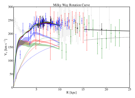
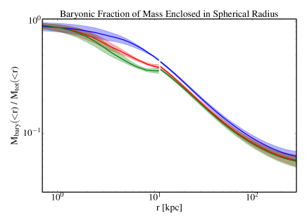
Oort’s constants. Traditionally, Oort’s constants and were defined for the local disk as a means to estimate the circular velocity and its gradient from radial velocity and PM data for nearby stellar populations, viz.
| (4) |
The quantity has been measured by many authors for different stellar populations (Feast & Whitelock, 1997; Uemura et al., 2000; Elias, Alfaro & Cabrera-Caño, 2006) with values in the range . For the rotation gradient , different authors find positive, zero and negative values. Catena & Ullio (2010) argue for from an sdss study of M stars (Fuchs et al., 2009).
6.4.3 Rotation curve
Figure 16 assembles rotation velocity measurements from various sources as explained in the caption. The data indicate a nearly flat rotation curve in the range (Reid et al., 2014) with a slight decrease at larger radii (Küpper et al., 2015; Kafle et al., 2012). PM data from gaia will clarify this. The rotation velocities determined by Sofue, Honma & Omodaka (2009, see also original references therein) from terminal velocities and a circular rotation model are unreliable in the region dominated by the Galactic bar (e.g., Englmaier & Gerhard, 1999; Fux, 1999), as is clearly visible in the central . Points inside (the half-length of the Galactic bar, §4.3) are therefore plotted in light shade.
Is the disk maximal? As shown with the illustrative models in Fig. 16, the answer to this question largely depends on the disk (mass) scalelength. These models include a bulge with dynamical mass fitted to the brava kinematic data and stellar mass corresponding to a Kroupa IMF (Portail et al., 2015). The disk has local stellar surface density (Bovy & Rix, 2013) and scalelengths (Bissantz & Gerhard, 2002; Bovy & Rix, 2013), (Robin et al., 2003; Jurić et al., 2008) and (Kent, Dame & Fazio, 1991; Gould, Bahcall & Flynn, 1996) and includes a gas disk with surface density and twice the stellar scalelength. A short scalelength has important implications: the Galaxy’s disk (summed over all stellar and gaseous components) is then maximal (Sackett, 1997) in the sense that the disk and bulge dominate the rotation curve, i.e. contribute of the rotational velocity and of the rotational support at . We included the bulge in the definition here because it mostly originates from the disk, §4.2. For the three scalelengths shown, the baryonic component provides a median fraction () of the circular velocity and ( of the radial force at . Thus the Milky Way’s disk is maximal only for the shortest scalelength (see also Sackett, 1997; Gerhard, 1999; Bovy & Rix, 2013; Piffl et al., 2014a), but even for the longer its contribution to the rotational velocity is at the upper limit of that inferred for typical spiral galaxies by Martinsson et al. (2013, -0.7), but see Aniyan et al. (2016).
6.4.4 Baryonic mass fraction with radius
The dynamical models shown in Fig. 16 have median total stellar masses of (. Of this, the stellar mass of the bulge and the disk embedded in the bulge region is . The remaining mass is consistent with the total disk mass given in Section 5, if we consider the mass of the long bar () as part of the disk mass. Thus our estimate of the total stellar mass in the MilkyWay is . Adding the mass in cold gas and the in hot gas resulting from Tepper-Garcia, Bland-Hawthorn & Sutherland (2015) for the NFW halo shown in Fig. 16 (, §6.3, ), the total baryonic mass fraction of the Galaxy becomes again . The resulting total baryonic mass fraction within radius from stars, cold gas, and hot gas is shown in Fig. 17.
, total stellar mass of the Galaxy
7 CONCLUDING REMARKS
The ultimate goal of Galactic research is to understand how the Milky Way has evolved from cosmological initial conditions to its present state, and how its future evolution will proceed. Our first task is to describe its current state in some detail; this allows us to connect to similar galaxies nearby and to studies of galaxies at high redshift. Characterizing the Galaxy’s dominant components and measuring their main parameters is an important step in this process.
The last few years have seen significant progress in several areas, driven by the impressive data from past and on-going surveys such as sdss, vvv, apogee and rave. We now have a quantitative description of the box/peanut structure of the Galactic bulge and, to a lesser extent, of its continuation into the Galactic plane, the long bar. We know that the thin and thick disks are distinct sequences in abundance ratios and age. The velocity field in the disk near the Sun has been charted, and dynamical models have been developed to link these data self-consistently to the gravitational potential. In the Galactic halo, multiple satellites and substructures have been discovered and density and velocity measurements have been made to beyond . On the other hand, we still lack good understanding of, e.g., the radial scale-length of the large-scale Galactic disk, the transition region between the Galactic bar and the surrounding disk, the properties of the nuclear disk, the mass of the stellar halo, and the outer rotation curve of the Milky Way. Constructing a complete structural model for the Milky Way is one of the main challenges for the coming years.
Half of all stars in the Universe formed before a redshift of unity. Detailed chemistry for millions of stars will provide important new information on the early formation of the different components. Until recently, most of our understanding of stars has come from the solar neighbourhood, but high-resolution stellar surveys have now begun to reach more representative regions of the Galaxy. We still do not have a complete chemical inventory for any component over its full physical extent. In principle, such data for enough stars will enable chemical tagging of dynamically distinct sub-systems. If even a few disrupted stellar systems with different ages can be recovered, we can learn about the role of secular evolution and stellar migration over cosmic time from their dispersal across the disk (Bland-Hawthorn, Krumholz & Freeman, 2010). But accurate elemental abundances are hampered by the difficulty of measuring good stellar parameters (e.g. log-g, effective temperature). The differential abundance technique shows great promise but this works best if the stars have a similar spectral type, thereby limiting the sample size. But we are encouraged by the revolution that is now under way to improve the state of the art in achieving consistent stellar abundances (Jofré et al., 2014; Ness et al., 2015).
We are looking forward to a golden age for Galactic research exemplified by ESA gaia, the astrometric space mission that was successfully deployed at the end of 2013. The ongoing or upcoming deep all-sky photometric (des, lsst, jwst, wfirst), spectroscopic (apogee-2, galah, weave, pfs, 4most) and seismological surveys (corot, k2, tess, plato) are well placed to advance our understanding of stellar populations. The large and extremely large telescopes will also play an important role, particularly with high-resolution spectroscopy (e.g. moons on vlt, g-clef on gmt).
The lsst co-added survey will reach up to four magnitudes deeper than SDSS: for stars with and , lsst will achieve a metallicity error of 0.1 dex for metal-rich stars and 0.2 dex for metal-poor stars for about 200 million F/G main sequence stars (Ivezić et al., 2008). In a single exposure, lsst will detect metal-poor MSTO stars to 140 kpc and horizontal branch stars and RR Lyrae to 500 kpc, going several times further in the final co-added data. lsst will also provide proper-motion measurements and parallaxes for stars below where gaia lacks sensitivity (Ivezić, Beers & Jurić, 2012). This will revolutionize photometric parallax and metallicity studies such as reviewed in §4.
The gaia astrometric mission will be even more far reaching for Galactic research. gaia will have an enormous impact on our understanding of 6D phase space (x, v) for the stars, particularly in the near field, but with important new information for giants extending into the outer halo. By the end of the decade, it will have obtained positions and velocities for up to two billion stars, i.e. phase space information for a few percent of stars that dominate the visible light in the Galaxy. In Fig. 18(left), many F/G dwarfs to be observed by lsst will have distances and proper motions with 10% accuracy out to kpc from the Sun. Moreover, in Fig. 18(right), dwarfs brighter than will have transverse velocities at least as good as the measured radial velocities. Such precise 6D phase space information will allow us to unravel the complex chemistry and dynamics of the local disk components to unprecedented levels.
Putting all the different strands together is not going to be easy. Increasingly sophisticated dynamical methods will be needed to accommodate the 6D phase space information in a complex multi-component potential, and to combine this with the chemical information ([Fe/H],[/Fe], …), but good progress is already being made (Hunt & Kawata, 2014; Sanders & Binney, 2015). Eventually, we will need to consider the departures from dynamical equilibrium which arise from internal evolution and interactions with the outside (Binney, 2013).
The Galaxy resembles a complex organism which evolves in a self-regulated fashion according to the laws of gravity, star formation, dynamics, and chemical evolution, while subject to mass accretion and external influences from its cosmological neighbourhood. Its low gas content, position in the green valley of the colour-magnitude diagram, and secularly evolved central parts of old stars indicate that it is in its late stages of evolution.
N-body and hydrodynamic simulations are becoming increasingly useful to help understand both formation and evolutionary processes (Stinson et al., 2013; Minchev, Chiappini & Martig, 2014; Feng et al., 2016; Scannapieco et al., 2015). These simulations will need to continue to grow in size to resolve smaller particle masses in both gas and dark matter, and to ultimately resolve individual star clusters. More thought must be given to how we “evaluate” the goodness of fit of a complex dynamical model, or a numerical simulation, when comparing to the high-dimensional data space available to Galactic researchers (Sharma et al., 2011). Through these comparisons Galactic studies will improve galaxy formation simulations and lead to a understanding of galaxy formation processes in general.
Ultimately, we may never arrive at a complete understanding of the Galaxy, much like any complex physical system. Most often, we learn about the physical laws through a series of approximations that become progressively more refined. But our search for understanding is noble all the same as we seek answers to the many wonders around us.
8 ONLINE VERSION: Analytic framework for fitting a parametric model to the Galaxy
We describe an analytic framework to model the Galaxy that is defined by a large set of kinematic parameters (Sharma et al., 2014). The framework is designed for rapid Bayesian optimization (e.g. Catena & Ullio, 2010) and shares important features with most studies of this kind (e.g. Rix & Bovy, 2013). The stellar content is modelled as a set of distinct components: the thin disk, the thick disk, the stellar halo and the bulge. The distribution functions, i.e., the number density of stars as a function of position (), velocity (), age (), metallicity (), and mass () for each component, is assumed to be specified a priori as a function where runs over the four components. The form of that correctly describes all the properties of the Galaxy and is self-consistent is still an open question.
For a given Galactic component, we assume stars form at a rate with a mass distribution (IMF) that is a function of age , where the present day spatial distribution of stars is conditional on age only. For a velocity distribution and metallicity distribution , we have
| (5) |
The functions take different forms for each Galactic component (Sharma et al., 2011). The IMF is normalized such that and is the mean stellar mass. The metallicity distribution is modeled as a log-normal distribution,
| (6) |
the mean and dispersion of which are given by age-dependent functions and . The is widely referred to as the age-metallicity relation (AMR). For the thin disk, the well known “age-scale height” relation is given by the axis ratio , viz.
| (7) |
Kinematic model. For a useful kinematic model, we want to constrain the velocity distribution . We assume that everything except for on the rhs of Eq. (5) is known. The functional form for is restricted because the spatial density distribution and the kinematics are linked to each other via the potential. The accuracy of a pure kinematic model depends upon our ability to supply functional forms of that are a good approximation to the actual velocity distribution of the system. A proper way to handle this problem would be to use dynamically self consistent models, but such models are still under development. Here we explore kinematic models that provide a reasonable approximation to the actual velocity distribution.
Gaussian velocity ellipsoid model. In this model, the velocity distribution is assumed to be a triaxial Gaussian,
| (8) |
where are cylindrical coordinates. The is the asymmetric drift and is given by
| (9) |
This follows from Eq. 4.227 in Binney & Tremaine (2008) assuming . This is valid for the case where the principal axes of velocity ellipsoid are aligned with the spherical coordinate system. If the velocity ellipsoid is aligned with the cylindrical coordinate system, then . Recent results using the RAVE data suggest that the velocity ellipsoid is aligned with the spherical coordinates (Siebert et al., 2008; Binney et al., 2014). One can parametrize our ignorance by writing the asymmetric drift as follows:
| (10) |
This is the form used by Bovy & Tremaine (2012).
The dispersions of the and components of velocity increase as a function age due to secular heating in the disk, and there is a radial dependence such that the dispersion increases towards the Galactic Center. We model these effects after Aumer & Binney (2009) using the functional form
| (11) | |||||
| (12) |
The choice of the radial dependence is motivated by the desire to produce disks in which the scale height is independent of radius. For example, under the epicyclic approximation, if is assumed to be constant, then the scale height is independent of radius for (van der Kruit & Freeman, 2011). In reality there is also a dependence of velocity dispersions which we have chosen to ignore in our present analysis. This means that for a given mono age population the asymmetric drift is independent of . However, the velocity dispersion and asymmetric drift of the combined population of stars are functions of . This is because the scale height of stars for a given isothermal population is an increasing function of its vertical velocity dispersion.
Shu distribution function model. The Gaussian velocity ellipsoid model has its limitations. In particular, the distribution of is strongly non-Gaussian, being highly skew to low . For a two-dimensional disk, a much better approximation to the velocity distribution is provided by the Shu (1969) distribution function. Moreover, the Shu DF, being dynamical in nature, connects the radial and azimuthal components of velocity dispersion to each other and to the mean-streaming velocity, thus lowering the number of free parameters in the model.
Assuming the potential is separable as we can write the distribution function as
where is the angular momentum,
| (13) | |||||
| (14) |
with
| (15) |
being the effective potential. Let be the radius of a circular orbit with specific angular momentum . In Schönrich (2012) (q.v. Sharma & Bland-Hawthorn, 2013), it was shown that the joint distribution of and can be written as
| (16) |
where is a function that controls the disk’s surface density and
| (17) | |||||
| (18) |
We assume to be specified as
| (19) |
and to be specified as
| (20) |
Now this leaves us to choose . This should be done so as to produce disks that satisfy the observational constraint given by , i.e., an exponential disk (or disks) with scale length . A simple way to do this is to let
| (21) |
However, this matches the target surface density only approximately. An alternative approach is to use the fast optimization formula proposed in Sharma & Bland-Hawthorn (2013) such that
| (22) |
where and is a function of the following form
| (23) |
with .
The gravitational potential . So far we have described kinematic models in which the potential is separable in and . In such cases, the energy associated with the vertical motion can be assumed to be the third integral of motion. In reality, the potential generated by a double exponential disk is not separable in and . For example, the hypothetical circular speed defined as can have both a radial and a vertical dependence, i.e.
| (24) |
The parameters and control the radial and vertical dependencies, respectively. The motivation for the vertical term comes from the fact that the above formula with provides a good fit to the profile of Milky Way potential (Dehnen & Binney, 1998; Law & Majewski, 2010). Both references have bulge, halo and disk components. The former has two double exponential disks while the later has a Miyamoto-Nagai disk.
To model systems where the potential is not separable in and , a simpler approach is motivated by the fact that, for realistic Galactic potentials, we expect the of a single age population to fall with . Binney (2012) finds that when vertical motion is present, the effective potential for radial motion (see Eq. 15) needs to be modified because the vertical motion also contributes to the centrifugal potential. Neglecting this effect leads to an overestimation of . As one moves away from the plane, this effect becomes increasingly important. Furthermore, as shown by Schönrich (2012), in a given solar annulus, stars with smaller will have larger vertical energy and hence larger scale height. Moreover, stars with smaller are more likely to be found at higher , consequently should also decrease with height.
The fall of with height is also predicted by the Jeans equation for an axisymmetric system
| (25) |
The at high will be lower both because is lower and because the term in the third square bracket decreases with , e.g., assuming .
For the Gaussian model, Sharma et al. (2014) simulate the overall reduction of with by introducing a parametrized form for as given by Eq. (24) in Eq. (9). Given this prescription we expect , so as to account for effects other than that involving the first term in Eq. (25). In reality, the velocity dispersion tensor will have a more complicated dependence on and than the exponential dependence on .
For the Shu model, Sharma et al. (2014) replace in Eq. (17) by the form in Eq. (24). However, the prescription breaks the dynamical self-consistency of the model and turns it into a fitting formula. In reality, the may not exactly follow the functional form for the vertical dependence predicted by our model, but is better than completely neglecting it.
DISCLOSURE STATEMENT
The authors are not aware of any conflicts that might be perceived as affecting the objectivity of this review.
ACKNOWLEDGMENTS
The initial idea for a review on the Galaxy’s global and structural parameters came from John Kormendy. It has been challenging to write not least because this is a vibrant and dynamic field of research, and major uncertainties still exist. But our motto throughout keep calm and carry on has sustained us even when no clear picture has emerged at times. Inevitably, with imposed page limits, there will be missing topics and references for which we apologize in advance. We thank our referee Tim Beers for his oversight of the review, and Ken Freeman, Rosie Wyse and James Binney for their historical perspective, wisdom and insight. We are indebted to various colleagues for their support and help with figures and tables: C. Correa, P. Kafle, T. Licquia, F. Mignard, Y. Momany, M. Portail, J. Read, T. Tepper-Garcia, D. Webster, C. Wegg, and for additional advice, perspectives and comments: M. Arnaboldi, B. Benjamin, T. Bensby, J. Bovy, M. Boylan-Kolchin, R. Drimmel, S. Gillessen, Z. Ivezic, R. Lange, P. McMillan, D. Nataf, M. Reid, R. Schödel and R. Schönrich. JBH acknowledges the Kavli Institute, UC Santa Barbara for their hospitality during the early planning of this review. JBH is supported by an ARC Australian Laureate Fellowship. OG is grateful for the support of the Max Planck Institute for Extraterrestrial Physics, and acknowledges a visiting fellowship from the Hunstead Fund for Astrophysics at the University of Sydney and the hospitality of Mount Stromlo Observatory during the final stages of the review.
References
- Abadi et al. (2010) Abadi M, Navarro J, Fardal M, Babul A, Steinmetz M. 2010. MNRAS 407:435
- Abadi, Navarro & Steinmetz (2006) Abadi MG, Navarro JF, Steinmetz M. 2006. MNRAS 365:747
- Adibekyan et al. (2012) Adibekyan VZ, Santos NC, Sousa SG, Israelian G, Delgado Mena E, et al. 2012. A&A 543:89
- Aguerri et al. (2015) Aguerri AL, Méndez-Abreu J, Falcón-Barroso J, Amorin A, Barrera-Ballesteros J, et al. 2015. A&A 576:A102
- Aguerri, Debattista & Corsini (2003) Aguerri JAL, Debattista VP, Corsini EM. 2003. MNRAS 338:465
- Aihara et al. (2011) Aihara H, Allende Prieto C, An D, Anderson S, Aubourg É, et al. 2011. ApJS 193:29
- Alard (2001) Alard C. 2001. A&A 379:L44
- Allende Prieto et al. (2008) Allende Prieto C, Majewski S, Schiavon R, Cunha K, Frinchaboy P, et al. 2008. Astronomische Nachrichten 329:1018
- Allgood et al. (2006) Allgood B, Flores R, Primack J, Kravtsov A, Wechsler R, et al. 2006. MNRAS 367:1781
- Alves-Brito et al. (2010) Alves-Brito A, Meléndez J, Asplund M, Ramírez I, Yong D. 2010. A&A 513:A35
- Anderson & Bregman (2010) Anderson M, Bregman J. 2010. ApJ 714:320
- Anderson & Bregman (2011) Anderson M, Bregman J. 2011. ApJ 737:22
- Anguiano et al. (2015) Anguiano B, Zucker DB, Scholz RD, Grebel EK, Seabroke G, et al. 2015. MNRAS 451:1229
- Aniyan et al. (2016) Aniyan S, Freeman KC, Gerhard OE, Arnaboldi M, Flynn C. 2016. MNRAS 456:1484
- Antoja et al. (2014) Antoja T, Helmi A, Dehnen W, Bienaymé O, Bland-Hawthorn J, et al. 2014. A&A 563:A60
- Antonini et al. (2012) Antonini F, Capuzzo-Dolcetta R, Mastrobuono-Battisti A, Merritt D. 2012. ApJ 750:111
- Arnadottir et al. (2009) Arnadottir AS, Feltzing S & Lundstrom I. 2009. IAU Symp 254:5
- Athanassoula (1992) Athanassoula E. 1992. MNRAS 259:328
- Athanassoula (2005) Athanassoula E. 2005. MNRAS 358:1477
- Aumer & Binney (2009) Aumer M, Binney JJ. 2009. MNRAS 397:1286
- Aumer & Schönrich (2015) Aumer M, Schönrich R. 2015. MNRAS 454:3166
- Babusiaux & Gilmore (2005) Babusiaux C, Gilmore G. 2005. MNRAS 358:1309
- Babusiaux et al. (2010) Babusiaux C, Gómez A, Hill V, Royer F, Zoccali M, et al. 2010. A&A 519:A77
- Bahcall & Soneira (1980) Bahcall J, Soneira R. 1980. ApJS 44:73
- Bailin et al. (2005) Bailin J, Kawata D, Gibson B, Steinmetz M, Navarro J, et al. 2005. ApJ 627:L17
- Bajkova & Bobylev (2015) Bajkova AT, Bobylev VV. 2015. Balt Astron 24:43
- Balick & Brown (1974) Balick B, Brown RL. 1974. ApJ 194:265
- Bartko et al. (2009) Bartko H, Martins F, Fritz TK, Genzel R, Levin Y, et al. 2009. ApJ 697:1741
- Battaglia et al. (2005) Battaglia G, Helmi A, Morrison H, Harding P, Olszewski EW, et al. 2005. MNRAS 364:433
- Beaulieu et al. (2000) Beaulieu SF, Freeman KC, Kalnajs AJ, Saha P, Zhao H. 2000. AJ 120:855
- Becklin & Neugebauer (1968) Becklin EE, Neugebauer G. 1968. ApJ 151:145
- Beers et al. (2012) Beers TC, Carollo D, Ivezić Ž, An D, Chiba M, et al. 2012. ApJ 746:34
- Bell et al. (2008) Bell EF, Zucker DB, Belokurov V, Sharma S, Johnston KV, et al. 2008. ApJ 680:295
- Beloborodov et al. (2006) Beloborodov AM, Levin Y, Eisenhauer F, Genzel R, Paumard T, et al. 2006. ApJ 648:405
- Belokurov et al. (2007) Belokurov V, Evans NW, Bell EF, Irwin MJ, Hewett PC, et al. 2007. ApJ 657:L89
- Belokurov et al. (2013) Belokurov V, Koposov SE, Evans NW, Penarrubia J, Irwin MJ, et al. 2013. MNRAS 437:116
- Belokurov et al. (2006) Belokurov V, Zucker DB, Evans NW, Gilmore G, Vidrih S, et al. 2006. ApJ 642:L137
- Benjamin et al. (2005) Benjamin R, Churchwell E, Babler B, Indebetouw R, al. E. 2005. ApJ 630:L149
- Bensby (2014) Bensby T. 2014. A&A 562:A71
- Bensby et al. (2010) Bensby T, Alves-Brito A, Oey M, Yong D, Meléndez J. 2010. A&A 516:L13
- Bensby et al. (2011) Bensby T, Alves-Brito A, Oey M, Yong D, Meléndez J. 2011. ApJ 735:L46
- Bensby, Feltzing & Lundström (2003) Bensby T, Feltzing S, Lundström I. 2003. A&A 410:527
- Bensby et al. (2009) Bensby T, Johnson J, Cohen J, Feltzing S, Udalski A, et al. 2009. A&A 499:737
- Bensby et al. (2007) Bensby T, Oey M, Feltzing S, Gustafsson B. 2007. ApJ 655:L89
- Bensby et al. (2013) Bensby T, Yee J, Feltzing S, Johnson J, Gould A, et al. 2013. A&A 549:A147
- Benson et al. (2003) Benson A, Bower R, Frenk C, Lacey C, Baugh C, Cole S. 2003. ApJ 599:38
- Bica et al. (2006) Bica E, Bonatto C, Barbuy B, Ortolani S. 2006. A&A 450:105
- Bienayme, Robin & Creze (1987) Bienayme O, Robin A, Creze M. 1987. A&A 180:94
- Binney & Tremaine (2008) Binney, J., & Tremaine, S. 2008, Galactic Dynamics: Second Edition, by James Binney and Scott Tremaine. ISBN 978-0-691-13026-2 (HB). Published by Princeton University Press, Princeton, NJ USA.
- Binney (2010) Binney J. 2010. MNRAS 401:2318
- Binney (2012) Binney J. 2012. MNRAS 426:1328
- Binney (2013) Binney J. 2013. New Astronomy Reviews 57:29
- Binney et al. (2014) Binney J, Burnett B, Kordopatis G, Steinmetz M, Gilmore G, et al. 2014. MNRAS 439:1231
- Binney, Gerhard & Spergel (1997) Binney J, Gerhard O, Spergel D. 1997. MNRAS 288:365
- Binney et al. (1991) Binney J, Gerhard OE, Stark AA, Bally J, Uchida KI. 1991. MNRAS 252:210
- Binney & McMillan (2011) Binney J, McMillan P. 2011. MNRAS 413:1889
- Binney & Piffl (2015) Binney, J., & Piffl, T. 2015, MNRAS, 454:3653
- Bird & Flynn (2015) Bird SA, Flynn C. 2015. MNRAS 452:2675
- Bissantz, Englmaier & Gerhard (2003) Bissantz N, Englmaier P, Gerhard O. 2003. MNRAS 340:949
- Bissantz & Gerhard (2002) Bissantz N, Gerhard O. 2002. MNRAS 330:591
- Blaauw et al. (1959) Blaauw A, Gum CS, Pawsey JL, Westerhout G. 1959. ApJ 130:702
- Blaauw et al. (1960) Blaauw A, Gum CS, Pawsey JL, Westerhout G. 1960. MNRAS 121:123
- Bland-Hawthorn & Cohen (2003) Bland-Hawthorn J & Cohen M. 2003. ApJ 582:246
- Bland-Hawthorn, Krumholz & Freeman (2010) Bland-Hawthorn J, Krumholz M, Freeman K. 2010. ApJ 713:166
- Bland-Hawthorn et al. (2005) Bland-Hawthorn J, Vlajić M, Freeman K, Draine B. 2005. ApJ 629:239
- Blanton & Moustakas (2009) Blanton M, Moustakas J. 2009. ARA&A 47:159
- Blanton & Roweis (2007) Blanton M, Roweis S. 2007. AJ 133:734
- Blitz & Robishaw (2000) Blitz L, Robishaw T. 2000. ApJ 541:675
- Bobylev (2013) Bobylev VV. 2013. Astron Lett 39:95
- Böker (2010) Böker T. 2010. IAU Symp 266:58
- Bonaca et al. (2012) Bonaca A, Jurić M, Ivezić Ž, Bizyaev D, Brewington H, et al. 2012. AJ 143:105
- Bond et al. (2010) Bond NA, Ivezić Ž, Sesar B, Jurić M, Munn JA, et al. 2010. ApJ 716:1
- Bottema (1993) Bottema R. 1993. A&A 275:16
- Bovy et al. (2015) Bovy J, Bird JC, Pérez AEG, Majewski SR, Nidever DL, Zasowski G. 2015. ApJ 800:83
- Bovy & Rix (2013) Bovy J, Rix HW. 2013. ApJ 779:115
- Bovy et al. (2012d) Bovy J, Allende Prieto C, Beers TC, Bizyaev D, da Costa LN, et al. 2012d. ApJ 759:131
- Bovy, Rix & Hogg (2012a) Bovy J, Rix HW, Hogg DW. 2012a. ApJ 751:131
- Bovy et al. (2012b) Bovy J, Rix HW, Liu C, Hogg DW, Beers TC, Lee YS. 2012b. ApJ 753:148
- Bovy & Tremaine (2012) Bovy J, Tremaine S. 2012. ApJ 756:89
- Bower et al. (2004) Bower GC, Falcke H, Herrnstein RM, Zhao JH, Goss WM, Backer DC. 2004. Science 304:704
- Bregman & Lloyd-Davies (2007) Bregman J, Lloyd-Davies E. 2007. ApJ 669:990
- Brook et al. (2012) Brook C, Stinson G, Gibson B, Kawata D, House E, et al. 2012. MNRAS 426:690
- Bryan & Norman (1998) Bryan GL & Norman, ML. 1998. ApJ 495:80
- Buchholz, Schödel & Eckart (2009) Buchholz RM, Schödel R, Eckart A. 2009. A&A 499:483
- Bullock & Johnston (2005) Bullock JS, Johnston KV. 2005. ApJ 635:931
- Bureau et al. (2006) Bureau M, Aronica G, Athanassoula E, Dettmar RJ, Bosma A, Freeman KC. 2006. MNRAS 370:753
- Burnett et al. (2011) Burnett B, Binney J, Sharma S, Williams M, Zwitter T, et al. 2011. A&A 113:14
- Burton (1988) Burton WB. 1988. Galactic and extragalactic radio astronomy (2nd Ed), Berlin New York, 295
- Cabrera-Lavers, Garzón & Hammersley (2005) Cabrera-Lavers A, Garzón F, Hammersley P. 2005. A&A 433:173
- Cabrera-Lavers et al. (2008) Cabrera-Lavers A, González-Fernández C, Garzón F, Hammersley P, López-Corredoira M. 2008. A&A 491:781
- Cabrera-Lavers et al. (2007) Cabrera-Lavers A, Hammersley P, González-Fernández C, López-Corredoira M, al. E. 2007. A&A 465:825
- Calamida et al. (2015) Calamida A, Sahu KC, Casertano S, Anderson J, Cassisi S, et al. 2015. ApJ 810:8
- Cao et al. (2013) Cao L, Mao S, Nataf D, Rattenbury NJ, Gould A. 2013. MNRAS 434:595
- Carney & Seitzer (1993) Carney B, Seitzer P. 1993. AJ 105:2127
- Carollo et al. (2007) Carollo D, Beers TC, Lee YS, Chiba M, Norris JE, et al. 2007. Nature 450:1020
- Carraro (2015) Carraro G. 2015. Bull. Assoc. Argentina Astron. 57:7
- Carraro et al. (2010) Carraro G, Vázquez RA, Costa E, Perren G, Moitinho A. 2010. ApJ 718:683
- Casagrande et al. (2011) Casagrande L, Schönrich R, Asplund M, Cassisi S, Ramírez I, et al. 2011. A&A 530:A138
- Catelan, Pritzl & Smith (2004) Catelan M, Pritzl BJ, Smith HA. 2004. ApJS 154:633
- Catena & Ullio (2010) Catena R, Ullio P. 2010. J Cosmol Astropart Phys 2010:4
- Cautun et al. (2014) Cautun M, Frenk CS, van de Weygaert R, Hellwing WA, Jones BJT. 2014. MNRAS 445:2049
- Chabrier (2003) Chabrier G. 2003. Publ Astron Soc Pacific 115:763
- Chakrabarty (2007) Chakrabarty D. 2007. A&A 467:145
- Chatzopoulos et al. (2015) Chatzopoulos S, Fritz TK, Gerhard O, Gillessen S, Wegg C, et al. 2015. MNRAS 447:948
- Chen et al. (1999) Chen B, Figueras F, Torra J, Jordi C, Luri X, Galadí-Enríquez D. 1999 A&A 352:459
- Chen et al. (2001) Chen B, Stoughton C, Smith JA, Uomoto A, Pier JR, et al. 2001. ApJ 553:184
- Cheng et al. (2012) Cheng J, Rockosi C, Morrison H, Lee Y, Beers T, et al. 2012. ApJ 752:51
- Chomiuk & Povich (2011) Chomiuk L, Povich M. 2011. AJ 142:197
- Clarkson et al. (2008) Clarkson W, Sahu K, Anderson J, Smith T, Brown T, et al. 2008. ApJ 684:1110
- Combes et al. (1990) Combes F, Debbasch F, Friedli D, Pfenniger D. 1990. A&A 233:82
- Comerón et al. (2012) Comerón S, Elmegreen, BG, Salo H et al. 2012. ApJ 759:98
- Conti & Vacca (1990) Conti PS, Vacca WD. 1990. AJ 100:431
- Contopoulos (1980) Contopoulos G. 1980. A&A 81:198
- Cooper et al. (2010) Cooper AP, Cole S, Frenk CS, White SDM, Helly J, et al. 2010. MNRAS 406:744
- Cooper et al. (2015) Cooper AP, Parry OH, Lowing B, Cole S, Frenk C. 2015. MNRAS 454:3185
- Correa et al. (2015) Correa C, Wyithe J, Schaye J, Duffy A. 2015. MNRAS 452:1217
- Cox & Loeb (2008) Cox T, Loeb A. 2008. MNRAS 386:461
- Crain et al. (2010) Crain R, McCarthy I, Frenk C, Theuns T, Schaye J. 2010. MNRAS 407:1403
- Cravens, Robertson & Snowden (2001) Cravens T, Robertson I, Snowden S. 2001. J. Geophys. Res. 106:24883
- Cuddeford & Amendt (1992) Cuddeford P, Amendt P. 1992. MNRAS 256:166
- Dambis (2009) Dambis AK. 2009. MNRAS 396:553
- de Bruijne et al. (2015) de Bruijne J, Allen M, Azaz S, Krone-Martins A, Prod’homme T, Hestroffer D. 2015. A&A 576:A74
- De Lucia (2012) De Lucia G. 2012. Astron Nachrichten 333:460
- De Lucia & Helmi (2008) De Lucia G, Helmi A. 2008. MNRAS 391:14
- de Rossi et al. (2009) de Rossi M, Tissera P, De Lucia G, Kauffmann G. 2009. MNRAS 395:210
- De Silva et al. (2015) De Silva GM, Freeman KC, Bland-Hawthorn J, Martell S, de Boer EW, et al. 2015. MNRAS 449:2604
- de Vaucouleurs (1983) de Vaucouleurs G. 1983. ApJ 268:468
- de Vaucouleurs & Pence (1978) de Vaucouleurs G, Pence W. 1978. AJ 83:1163
- Deason, Belokurov & Evans (2011) Deason AJ, Belokurov V, Evans NW. 2011. MNRAS 416:2903
- Deason et al. (2012) Deason AJ, Belokurov V, Evans NW, An J. 2012. MNRAS 424:L44
- Deason et al. (2013) Deason AJ, Belokurov V, Evans NW, Johnston KV. 2013. ApJ 763:113
- Deason et al. (2014) Deason AJ, Belokurov V, Koposov SE, Rockosi CM. 2014. ApJ 787:30
- Debattista, Gerhard & Sevenster (2002) Debattista VP, Gerhard O, Sevenster MN. 2002. MNRAS 334:355
- Dehnen (1998) Dehnen W. 1998. AJ 115:2384
- Dehnen (2000) Dehnen W. 2000. AJ 119:800
- Dehnen & Binney (1998) Dehnen W, Binney JJ. 1998. MNRAS 298:387
- Dehnen et al. (2006) Dehnen, W., McLaughlin, D. E., & Sachania, J. 2006, MNRAS 369:1688
- Dékány et al. (2013) Dékány I, Minniti D, Catelan M, Zoccali M, Saito RK, et al. 2013. ApJ 776:L19
- Dékány et al. (2015) Dékány I, Minniti D, Majaess D, Zoccali M, Hajdu G, et al. 2015. ApJ 812:L29
- Delhaye (1965) Delhaye J. 1965. In Galactic Structure, 61 (eds. A Blaauw, M Schmidt)
- Deng et al. (2012) Deng LC, Newberg H, Liu C, Carlin J, Beers T, et al. 2012. Research in A&A 12:735
- Di Matteo et al. (2014) Di Matteo P, Haywood M, Gómez A, van Damme L, Combes F, et al. 2014. A&A 567:A122
- Diplas & Savage (1991) Diplas A, Savage B. 1991. ApJ 377:126
- Do et al. (2013) Do T, Martinez GD, Yelda S, Ghez A, Bullock J, et al. 2013. ApJ 779:L6
- Doeleman et al. (2008) Doeleman SS, Weintroub J, Rogers AEE, Plambeck R, Freund R, et al. 2008. Nature 455:78
- Drimmel & Spergel (2001) Drimmel R, Spergel D. 2001. ApJ 556:181
- Driver et al. (2011) Driver SP, Hill DT, Kelvin LS, Robotham ASG, Liske J, et al. 2011. MNRAS 413:971
- Dubinski & Carlberg (1991) Dubinski J, Carlberg R. 1991. ApJ 378:496
- Dwek et al. (1995) Dwek E, Arendt R, Hauser M, Kelsall T, al. E. 1995. ApJ 445:716
- Eckart & Genzel (1997) Eckart A, Genzel R. 1997. MNRAS 284:576
- Eckart et al. (1995) Eckart A, Genzel R, Hofmann R, Sams BJ, Tacconi-Garman LE. 1995. ApJ 445:L23
- Edvardsson et al. (1993) Edvardsson B, Andersen J, Gustafsson B, Lambert D, Nissen P, Tomkin J. 1993. A&A 275:101
- Efremov (2011) Efremov Y. 2011. Astronomy Reports 55:108
- Eggen (1951) Eggen O. 1951. ApJ 113:657
- Eggen, Lynden-Bell & Sandage (1962) Eggen OJ, Lynden-Bell D, Sandage AR. 1962. ApJ 136:748
- Eisenhauer et al. (2003) Eisenhauer F, Schdel R, Genzel R, Ott T, Tecza M, et al. 2003. ApJ 597:L121
- Elias, Alfaro & Cabrera-Caño (2006) Elias F, Alfaro EJ, Cabrera-Caño J. 2006. AJ 132:1052
- Ellis & Bland-Hawthorn (2007) Ellis SC, Bland-Hawthorn J. 2007. MNRAS 377:815
- Englmaier & Gerhard (1999) Englmaier P, Gerhard O. 1999. MNRAS 304:512
- Evans et al. (2016) Evans NW, Sanders JL, Williams AA, An J, Lynden-Bell D, Dehnen W. 2016. MNRAS 456:4506
- Faccioli et al. (2014) Faccioli L, Smith MC, Yuan HB, Zhang HH, Liu XW, et al. 2014. ApJ 788:105
- Fang, Bullock & Boylan-Kolchin (2013) Fang T, Bullock J, Boylan-Kolchin M. 2013. ApJ 762:20
- Feast & Whitelock (1997) Feast M, Whitelock P. 1997. MNRAS 291:683
- Feldmeier et al. (2014) Feldmeier A, Neumayer N, Seth A, Schödel R, Lützgendorf N, et al. 2014. A&A 570:A2
- Feng et al. (2016) Feng Y, Di Matteo TD, Croft R, Tenneti A, Bird S, Battaglia N. 2015. MNRAS 455:2778
- Fermani & Schönrich (2013) Fermani F, Schönrich R. 2013. MNRAS 432:2402
- Finlator et al. (2000) Finlator K, Ivezić Ž, Fan X, Strauss M, Knapp G, et al. 2000. AJ 120:2615
- Flynn et al. (2006) Flynn C, Holmberg J, Portinari L, Fuchs B, Jahreiss H. 2006. MNRAS 372:1149
- Font et al. (2006) Font AS, Johnston KV, Bullock JS, Robertson BE. 2006. ApJ 638:585
- Font et al. (2011) Font AS, McCarthy IG, Crain RA, Theuns T, Schaye J, et al. 2011. MNRAS 416:2802
- Forero-Romero et al. (2013) Forero-Romero JE, Hoffman Y, Bustamante S, Gottloeber S, Yepes G. 2013. ApJ 767:5
- Fox et al. (2014) Fox AJ, Wakker BP, Barger KA, Hernandez AK, Richter P, et al. 2014. ApJ 787:147
- Francis & Anderson (2014) Francis C, Anderson E. 2014. MNRAS 441:1105
- Freeman (2001) Freeman K. 2001. ASP Conf 230:91
- Freeman & Bland-Hawthorn (2002) Freeman K, Bland-Hawthorn J. 2002. Annu Rev A&A 40:487
- Freudenreich (1998) Freudenreich HT. 1998. ApJ 492:495
- Fritz et al. (2011) Fritz TK, Gillessen S, Dodds-Eden K, Lutz D, Genzel R, et al. 2011. ApJ 737:73
- Fritz et al. (2016) Fritz TK, Chatzopoulos S, Gerhard O, Gillessen S, Genzel R, et al. 2016. ApJ 821:44
- Fuchs et al. (2009) Fuchs B, Dettbarn C, Rix HW, Beers TC, Bizyaev D, et al. 2009. AJ 137:4149
- Fuhrmann (1998) Fuhrmann K. 1998. A&A 330:626
- Fuhrmann (2008) Fuhrmann K. 2008. MNRAS 384:173
- Fux (1999) Fux R. 1999. A&A 345:787
- Garbari et al. (2012) Garbari S, Liu C, Read JI, Lake G. 2012. MNRAS 425:1445
- Gatto et al. (2013) Gatto A, Fraternali F, Read J, Marinacci F, Lux H, Walch S. 2013. MNRAS 433:2749
- Genzel, Eisenhauer & Gillessen (2010) Genzel R, Eisenhauer F, Gillessen S. 2010. Rev Mod Phys 82:3121
- Genzel et al. (2000) Genzel R, Pichon C, Eckart A, Gerhard OE, Ott T. 2000. MNRAS 317:348
- Gerhard & Martinez-Valpuesta (2012) Gerhard O, Martinez-Valpuesta I. 2012. ApJ 744:L8
- Gerhard (1999) Gerhard OE. 1999. ASP Conf 182:307
- Ghez et al. (1998) Ghez AM, Klein BL, Morris M, Becklin EE. 1998. ApJ 509:678
- Ghez et al. (2008) Ghez AM, Salim S, Weinberg NN, Lu JR, Do T, et al. 2008. ApJ 689:1044
- Gibbons, Belokurov & Evans (2014) Gibbons SLJ, Belokurov V, Evans NW. 2014. MNRAS 445:3788
- Gillessen et al. (2009a) Gillessen S, Eisenhauer F, Fritz TK, Bartko H, Dodds-Eden K, et al. 2009a. ApJ 707:L114
- Gillessen et al. (2013) Gillessen S, Eisenhauer F, Fritz TK, Pfuhl O, Ott T, Genzel R. 2013. IAU Symp 289:29
- Gillessen et al. (2009b) Gillessen S, Eisenhauer F, Trippe S, Alexander T, Genzel R, et al. 2009b. ApJ 692:1075
- Gilmore et al. (2012) Gilmore G, Randich S, Asplund M, Binney J, Bonifacio P, et al. 2012. The Messenger 147:25
- Gilmore & Reid (1983) Gilmore G, Reid N. 1983. MNRAS 202:1025
- Gnedin et al. (2010) Gnedin, O. Y., Brown, W. R., Geller, M. J., & Kenyon, S. J. 2010, ApJ 720:L108
- Gonzalez et al. (2011a) Gonzalez O, Rejkuba M, Minniti D, Zoccali M, Valenti E, Saito R. 2011a. A&A 534:L14
- Gonzalez et al. (2012) Gonzalez O, Rejkuba M, Zoccali M, Valenti E, Minniti D, et al. 2012. A&A 543:A13
- Gonzalez & Gadotti (2016) Gonzalez OA, Gadotti DA. 2016. Astr Space Sci Lib 418:199
- Gonzalez et al. (2011b) Gonzalez OA, Rejkuba M, Zoccali M, Hill V, Battaglia G, et al. 2011b. A&A 530:A54
- Gonzalez et al. (2013) Gonzalez OA, Rejkuba M, Zoccali M, Valent E, Minniti D, Tobar R. 2013. A&A 552:A110
- Goodman et al. (2014) Goodman AA, Alves J, Beaumont CN, Benjamin RA, Borkin MA, et al. 2014. ApJ 797:53
- Gould, Bahcall & Flynn (1996) Gould A, Bahcall JN, Flynn C. 1996. ApJ 465:759
- Gratton et al. (2000) Gratton R, Carretta E, Matteucci F, Sneden C. 2000. A&A 358:671
- Grcevich & Putman (2009) Grcevich J, Putman M. 2009. ApJ 696:385
- Groenewegen, Udalski & Bono (2008) Groenewegen MAT, Udalski A, Bono G. 2008. A&A 481:441
- Groenewegen & Blommaert (2005) Groenewegen MAT, Blommaert JADL. 2005. A&A 443:143
- Guedes et al. (2013) Guedes J, Mayer L, Carollo M, Madau P. 2013. ApJ 772:36
- Gupta et al. (2012) Gupta A, Mathur S, Krongold Y, Nicastro F, Galeazzi M. 2012. ApJ 756:L8
- Habing (1988) Habing H. 1988. A&A 200:40
- Habing et al. (2006) Habing HJ, Sevenster MN, Messineo M, van de Ven G, Kuijken K. 2006. A&A 458:151
- Hammer et al. (2012) Hammer F, Puech M, Flores H et al. 2012. European Physical Journal Web of Conferences, 19:01004
- Hammersley et al. (2000) Hammersley P, Garzón F, Mahoney T, López-Corredoira M, Torres M. 2000. MNRAS 317:L45
- Harris (2010) Harris WE. 2010. arXiv:1012.3224
- Hartmann & Burton (1997) Hartmann D, Burton W. 1997. Atlas of Galactic Neutral Hydrogen.
- Hawkins et al. (2015) Hawkins K, Jofre P, Masseron T, Gilmore G. 2015. MNRAS 453:758
- Hayden et al. (2015) Hayden MR, Bovy J, Holtzman JA, Nidever DL, Bird JC, et al. 2015. ApJ 808:132
- Haywood (2006) Haywood M. 2006. MNRAS 371:1760
- Haywood et al. (2015) Haywood M, Matteo PD, Snaith O, Lehnert MD. 2015. A&A 579:5
- Haywood, Robin & Crézé (1997) Haywood M, Robin AC, Crézé M. 1997. A&A 320:428
- Helmi (2004) Helmi A. 2004. ApJ 610:L97
- Helmi (2008) Helmi A. 2008. A&ARev 15:145
- Henley & Shelton (2012) Henley D, Shelton R. 2012. ApJS 202:14
- Henley et al. (2010) Henley D, Shelton R, Kwak K, Joung M, Mac Low MM. 2010. ApJ 723:935
- Hill et al. (2011) Hill V, Lecureur A, Gómez A, Zoccali M, Schultheis M, et al. 2011. A&A 534:A80
- Hinshaw et al. (2003) Hinshaw G, Spergel D, Verde L, Hill R, Meyer S, et al. 2003. ApJS 148:135
- Holmberg et al. (2007) Holmberg, J., Nordström, B., & Andersen, J. 2007, A&A 475: 519
- Holmberg et al. (2009) Holmberg, J., Nordström, B., & Andersen, J. 2009, A&A 501: 941
- Honma et al. (2007) Honma M, Bushimata T, Choi YK, Hirota T, Imai H, et al. 2007. PASJ 59:889
- Honma et al. (2012) Honma M, Nagayama T, Ando K, Bushimata T, Choi YK, et al. 2012. PASJ 64:136
- Hopkins et al. (2014) Hopkins P, Kereš D, Oñorbe J, Faucher-Giguère CA, Quataert E, et al. 2014. MNRAS 445:581
- Humphreys & Larsen (1995) Humphreys RM, Larsen JA. 1995. AJ 110:2183
- Hunt & Kawata (2014) Hunt JAS, Kawata D. 2014. MNRAS 443:2112
- Ibata et al. (2003) Ibata R, Irwin M, Lewis G, Ferguson A, Tanvir N. 2003. MNRAS 340:L21
- Ibata et al. (2001) Ibata R, Lewis GF, Irwin M, Totten E, Quinn T. 2001. ApJ 551:294
- Ibata et al. (2013) Ibata R, Lewis GF, Martin NF, Bellazzini M, Correnti M. 2013. ApJ 765:L15
- Ibata et al. (1997) Ibata RA, Wyse RFG, Gilmore G, Irwin MJ, Suntzeff NB. 1997. AJ 113:634
- Irwin et al. (2005) Irwin M, Ferguson A, Ibata R, Lewis G, Tanvir N. 2005. ApJ 628:L105
- Ivezić, Beers & Jurić (2012) Ivezić Ž, Beers TC, Jurić M. 2012. Annu Rev A&A 50:251
- Ivezić et al. (2008) Ivezić Ž, Sesar B, Jurić M, Bond N, Dalcanton J, et al. 2008. ApJ 684:287
- Jofré et al. (2014) Jofré P, Heiter U, Soubiran C, Blanco-Cuaresma S, Worley C, et al. 2014. A&A 564:A133
- Johnson et al. (2011) Johnson CI, Rich MR, Fulbright JP, Valenti E, McWilliam A. 2011. ApJ 732:108
- Johnston, Law & Majewski (2005) Johnston KV, Law DR, Majewski SR. 2005. ApJ 619:800
- Jurić et al. (2008) Jurić M, Ivezić Ž, Brooks A, Lupton RH, Schlegel D, et al. 2008. ApJ 673:864
- Just & Jahreiss (2010) Just A, Jahreiss H. 2010. MNRAS 402:461
- Kafle et al. (2012) Kafle PR, Sharma S, Lewis GF, Bland-Hawthorn J. 2012. ApJ 761:98
- Kafle et al. (2014) Kafle, P. R., Sharma, S., Lewis, G. F., & Bland-Hawthorn, J. 2014. ApJ 794:59
- Kalberla & Dedes (2008) Kalberla PMW, Dedes L. 2008. A&A 487:951
- Kalberla et al. (2007) Kalberla PMW, Dedes L, Kerp J, Haud U. 2007. A&A 469:511
- Kalnajs (1991) Kalnajs AJ. 1991. Dynamics of Disc Galaxies, 323 (ed. B. Sundelius)
- Kapteyn (1922) Kapteyn J. 1922. ApJ 55:302
- Kazantzidis et al. (2004) Kazantzidis S, Kravtsov A, Zentner A, Allgood B, Nagai D, Moore B. 2004. ApJ 611:L73
- Kent (1992) Kent SM. 1992. ApJ 387:181
- Kent, Dame & Fazio (1991) Kent SM, Dame TM, Fazio G. 1991. ApJ 378:131
- Kerr & Lynden-Bell (1986) Kerr FJ, Lynden-Bell D. 1986. MNRAS 221:1023
- Kimmig et al. (2015) Kimmig B, Seth A, Ivans II, Strader J, Caldwell N, et al. 2015. AJ 149:53
- King et al. (2015) King C, Brown WR, Geller MJ, Kenyon SJ. 2015. ApJ 813:89
- Klypin et al. (2002) Klypin A, Zhao H & Somerville RS. 2002. ApJ 573:597
- Kobayashi et al. (2008) Kobayashi N, Yasui C, Tokunaga A, Saito M. 2008. ApJ 683:178
- Koposov, Rix & Hogg (2010) Koposov SE, Rix HW, Hogg DW. 2010. ApJ 712:260
- Kordopatis et al. (2015) Kordopatis G, Wyse RFG, Gilmore G, Recio-Blanco A, de Laverny P, et al. 2015. A&A 582:122
- Kormendy & Barentine (2010) Kormendy J, Barentine JC. 2010. ApJ 715:L176
- Kormendy et al. (2010) Kormendy J, Drory N, Bender R, Cornell M. 2010. ApJ 723:54
- Kormendy & Ho (2013) Kormendy J, Ho LC. 2013. Annu Rev A&A 51:511
- Kormendy (2013) Kormendy J. 2013. Secular Evolution in Disk Galaxies, XXIII Canary Islands Winter School of Astrophysics, ed. J. Falcon-Barroso & J. H. Knapen (Cambridge: Cambridge Univ. Press), p. 1.
- Krabbe et al. (1995) Krabbe A, Genzel R, Eckart A, Najarro F, Lutz D, et al. 1995. ApJ 447
- Kroupa (2001) Kroupa P. 2001. MNRAS 322:231
- Kuijken & Gilmore (1989) Kuijken K, Gilmore G. 1989. MNRAS 239:571
- Kunder et al. (2012) Kunder A, Koch A, Rich R, de Propris R, Howard C, et al. 2012. AJ 143:57
- Kunder et al. (2016) Kunder A, Rich RM, Koch A, Storm J, Nataf DM, et al. 2016. ApJ 821:L25
- Küpper et al. (2015) Küpper AHW, Balbinot E, Bonaca A, Johnston KV, Hogg DW, et al. 2015. ApJ 803:80
- Lacy et al. (1980) Lacy JH, Townes CH, Geballe TR, Hollenbach DJ. 1980. ApJ 241:132
- Lange et al. (2015) Lange R, Driver S, Robotham A, Kelvin L, Graham A, et al. 2015. MNRAS 447:2603
- Larsen & Humphreys (2003) Larsen JA, Humphreys RM. 2003. AJ 125:1958
- Launhardt, Zylka & Mezger (2002) Launhardt R, Zylka R, Mezger PG. 2002. A&A 384:112
- Laurikainen et al. (2014) Laurikainen E, Salo H, Athanassoula E, Bosma A, Herrera-Endoqui M. 2014. MNRAS 444:L80
- Laurikainen et al. (2011) Laurikainen E, Salo H, Buta R, Knapen JH. 2011. MNRAS 418:1452
- Law & Majewski (2010) Law DR, Majewski SR. 2010. ApJ 714:229
- Lewis & Freeman (1989) Lewis JR, Freeman KC. 1989. AJ 97:139
- Li & White (2008) Li YS, White SDM. 2008. MNRAS 384:1459
- Li & Shen (2012) Li ZY, Shen J. 2012. ApJ 757:L7
- Licquia & Newman (2015) Licquia TC, Newman JA. 2015. ApJ 806:96
- Licquia, Newman & Brinchmann (2015) Licquia TC, Newman JA, Brinchmann J. 2015, apj 809:96
- Lindqvist, Habing & Winnberg (1992) Lindqvist M, Habing HJ, Winnberg A. 1992. A&A 259:118
- Loebman et al. (2011) Loebman, S. R., Roškar, R., Debattista, V. P., et al. 2011, ApJ, 737:8
- Loebman et al. (2012) Loebman SR, Ivezić Ž, Quinn TR, Governato F, Brooks AM, et al. 2012. ApJ 758:L23
- Long et al. (2012) Long RJ, Mao S, Shen J, Wang Y. 2012. MNRAS 428:3478
- López-Corredoira (2014) López-Corredoira M. 2014. A&A 563:A128
- López-Corredoira et al. (2002) López-Corredoira M, Cabrera-Lavers A, Garzón F, Hammersley P. 2002. A&A 394:883
- López-Corredoira, Cabrera-Lavers & Gerhard (2005) López-Corredoira M, Cabrera-Lavers A, Gerhard O. 2005. A&A 439:107
- Lowing et al. (2014) Lowing B, Wang W, Cooper A, Kennedy R, Helly J, et al. 2014. MNRAS 446:2274
- Magrini et al. (2015) Magrini L, Randich S, Donati P, Bragaglia A, Adibekyan V, et al. 2015. A&A 580:A85
- Maíz-Apellániz (2001) Maíz-Apellániz J. 2001. AJ 121:2737
- Majaess (2010) Majaess D. 2010. Acta Astron 60:55
- Malhotra et al. (1996) Malhotra S, Spergel D, Rhoads J, Li J. 1996. ApJ 473:687
- Malkin (2013) Malkin Z. 2013. IAU Symp 289:406
- Martinez-Valpuesta & Gerhard (2013) Martinez-Valpuesta I, Gerhard O. 2013. ApJ 766:L3
- Martinsson et al. (2013) Martinsson TPK, Verheijen MAW, Westfall KB, Bershady MA, Andersen DR, Swaters RA. 2013. A&A 557:A131
- Masseron & Gilmore (2015) Masseron T, Gilmore G. 2015. MNRAS 453:1855
- Matsunaga et al. (2013) Matsunaga N, Feast MW, Kawadu T, Nishiyama S, Nagayama T, et al. 2013. MNRAS 429:385
- Matsunaga et al. (2009) Matsunaga N, Kawadu T, Nishiyama S, Nagayama T, Hatano H, et al. 2009. MNRAS 399:1709
- Matsunaga et al. (2011) Matsunaga N, Kawadu T, Nishiyama S, Nagayama T, Kobayashi N, et al. 2011. Nature 477:188
- May et al. (1993) May J, Bronfman L, Alvarez H, Murphy D, Thaddeus P. 1993. A&AS 99:105
- McCarthy et al. (2012) McCarthy IG, Font AS, Crain RA, Deason AJ, Schaye J, Theuns T. 2012. MNRAS 420:2245
- McKee & Williams (1997) McKee C, Williams J. 1997. ApJ 476:144
- McKee, Parravano & Hollenbach (2015) McKee CF, Parravano A, Hollenbach DJ. 2015. ApJ 814:1
- McMillan (2011) McMillan PJ. 2011 MNRAS 414:2446
- McWilliam & Zoccali (2010) McWilliam A, Zoccali M. 2010. ApJ 724:1491
- Mendez & van Altena (1998) Mendez RA, van Altena WF. 1998. A&A 330:910
- Merritt (2013) Merritt D. 2013. Dynamics and Evolution of Galactic Nuclei.
- Merritt, Berczik & Laun (2007) Merritt D, Berczik P, Laun F. 2007. AJ 133:553
- Mignard (2011) Mignard F. 2011. ftp://ftp.oca.eu/pub/mignard/TN_Gaia/GAIA-CA-TN-OCA-FM-048.pdf
- Mihalas & Binney (1981) Mihalas D, Binney J. 1981. Galactic Astronomy: Structure and Kinematics. (San Francisco: WH Freeman)
- Miller & Bregman (2013) Miller M, Bregman J. 2013. ApJ 770:118
- Miller & Bregman (2015) Miller M, Bregman J. 2015. ApJ 800:14
- Minchev, Chiappini & Martig (2014) Minchev I, Chiappini C, Martig M. 2014. A&A 572:A92
- Minchev & Famaey (2010) Minchev I & Famaey B. 2010. ApJ 722:112
- Minchev et al. (2015) Minchev I, Martig M, Streich D et al. 2015. ApJ 804:L9
- Minchev, Nordhaus & Quillen (2007) Minchev I, Nordhaus J, Quillen AC. 2007. ApJ 664:L31
- Minniti et al. (2010) Minniti D, Lucas PW, Emerson JP, Saito RK, Hempel M, et al. 2010. New Astronomy 15:433
- Minniti et al. (2011) Minniti D, Saito R, Alonso-García J, Lucas P, Hempel M. 2011. ApJ 733:L43
- Molinari et al. (2011) Molinari S, Bally J, Noriega-Crespo A, Compiègne M, Bernard JP, et al. 2011. ApJ 735:L33
- Momany et al. (2006) Momany Y, Zaggia S, Gilmore G, Piotto G, Carraro G, et al. 2006. A&A 451:515
- Moni Bidin, Carraro & Méndez (2012) Moni Bidin C, Carraro G, Méndez RA. 2012. ApJ 747:101
- Morris, Meyer & Ghez (2012) Morris MR, Meyer L, Ghez AM. 2012. Res A&A 12:995
- Morrison (1993) Morrison HL. 1993. AJ 106:578
- Munn et al. (2004) Munn J, Monet D, Levine S, Canzian B, Pier J, et al. 2004. AJ 127:3034
- Mutch, Croton & Poole (2011) Mutch SJ, Croton DJ, Poole GB. 2011. ApJ 736:84
- Nataf et al. (2010) Nataf DM, Udalski A, Gould A, Fouqué P, Stanek K. 2010. ApJ 721:L28
- Nataf et al. (2013) Nataf DM, Gould A, Fouqué P, Gonzalez OA, Johnson JA, et al. 2013. ApJ 769:88
- Nataf et al. (2015) Nataf DM, Udalski A, Skowron J, Szyma ski MK, Kubiak M, et al. 2015. MNRAS 447:1535
- Ness et al. (2012) Ness M, Freeman K, Athanassoula E, Wylie-De-Boer E, Bland-Hawthorn J, et al. 2012. ApJ 756:22
- Ness et al. (2013a) Ness M, Freeman K, Athanassoula E, Wylie-de-Boer E, Bland-Hawthorn J, et al. 2013a. MNRAS 430:836
- Ness et al. (2013b) Ness M, Freeman K, Athanassoula E, Wylie-de-Boer E, Bland-Hawthorn J, et al. 2013b. MNRAS 432:2092
- Ness et al. (2015) Ness M, Hogg D, Rix HW, Ho A, Zasowski G. 2015. ApJ 808:16
- Newberg et al. (2002) Newberg H, Yanny B, Rockosi C, Grebel E, Rix HW, et al. 2002. ApJ 569:245
- Nichols & Bland-Hawthorn (2011) Nichols M, Bland-Hawthorn J. 2011. ApJ 732:17
- Nidever et al. (2014) Nidever DL, Bovy J, Bird JC, Andrews BH, Hayden M, et al. 2014 ApJ 796:3
- Niederste-Ostholt et al. (2010) Niederste-Ostholt M, Belokurov V, Evans NW, Peñarrubia J. 2010. ApJ 712:516
- Nishiyama et al. (2005) Nishiyama S, Nagata T, Baba D, Haba Y, Kadowaki R, et al. 2005. ApJ 621:L105
- Nishiyama et al. (2006) Nishiyama S, Nagata T, Sato S, Kato D, Nagayama T, et al. 2006. ApJ 647:1093
- Nishiyama et al. (2008) Nishiyama S, Nagata T, Tamura M, Kandori R, Hatano H, et al. 2008. ApJ 680:1174
- Nishiyama et al. (2013) Nishiyama S, Yasui K, Nagata T, Yoshikawa T, Uchiyama H, et al. 2013. ApJ 769:L28
- Nissen & Schuster (2011) Nissen PE & Schuster WJ. 2011. A&A 530, A15
- Nordström et al. (2004) Nordström B, Mayor M, Andersen J, Holmberg J, Pont F, et al. 2004. A&A 418:989
- Norris & Ryan (1991) Norris J, Ryan S. 1991. ApJ 380:403
- Nuza et al. (2014) Nuza S, Parisi F, Scannapieco C, Richter P, Gottlöber S, Steinmetz M. 2014. MNRAS 441:2593
- Obreja et al. (2013) Obreja A, Domínguez-Tenreiro R, Brook C, Martínez-Serrano FJ, Doménech-Moral M, et al. 2013. ApJ 763:26
- Ojha (2001) Ojha DK. 2001. MNRAS 322:426
- Oort & Rougoor (1960) Oort JH, Rougoor GW. 1960. MNRAS 121
- Ortolani et al. (1995) Ortolani S, Renzini A, Gilmozzi R, Marconi G, Barbuy B, et al. 1995. Nature 377:701
- Paczynski & Stanek (1998) Paczynski B, Stanek KZ. 1998. ApJ 494:L219
- Paerels & Kahn (2003) Paerels F, Kahn S. 2003. ARA&A 41:291
- Pandey, Bhatt & Mahra (1988) Pandey AK, Bhatt BC, Mahra HS. 1988. A&A 189:66
- Parkinson, Cole & Helly (2008) Parkinson H, Cole S, Helly J. 2008. MNRAS 383:557
- Pasetto et al. (2012) Pasetto S, Grebel EK, Zwitter T, Chiosi C, Bertelli G, et al. 2012. Astron. Astrophys. 547:A70
- Patterson (1940) Patterson FS. 1940. Harvard College Observatory Bulletin 914:9
- Paumard et al. (2006) Paumard T, Genzel R, Martins F, Nayakshin S, Beloborodov AM, et al. 2006. ApJ 643:1011
- Peebles & Tully (2013) Peebles P, Tully R. 2013. arXiv:1302.6982
- Perryman, Spergel & Lindegren (2014) Perryman M, Spergel DN, Lindegren L. 2014. ApJ 789:166
- Pfenniger & Friedli (1991) Pfenniger D, Friedli D. 1991. A&A 252:75
- Pfuhl et al. (2011) Pfuhl O, Fritz TK, Zilka M, Maness H, Eisenhauer F, et al. 2011. ApJ 741:108
- Piddington & Minnett (1951) Piddington JH, Minnett HC. 1951. Aust J Sci Res A4:459
- Pietrukowicz et al. (2015) Pietrukowicz P, Kozlowski S, Skowron J, Soszynski I, Udalski A, et al. 2015. ApJ 811:113
- Piffl et al. (2014a) Piffl T, Binney J, McMillan PJ, Steinmetz M, Helmi A, et al. 2014a. MNRAS 445:3133
- Piffl et al. (2014b) Piffl T, Scannapieco C, Binney JJ, Steinmetz M, et al. 2014b. A&A 562:A91
- Pila-Díez et al. (2015) Pila-Díez B, de Jong JTA, Kuijken K, van der Burg RFJ, Hoekstra H. 2015. A&A 579:A38
- Pillepich, Madau & Mayer (2015) Pillepich A, Madau P, Mayer L. 2015. ApJ 799:184
- Pillepich et al. (2014) Pillepich A, Vogelsberger M, Deason A, Rodriguez-Gomez V, Genel S, et al. 2014. MNRAS 444:237
- Pipino, Matteucci & D’Ercole (2008) Pipino A, Matteucci F, D’Ercole A. 2008. IAU Symp 245:19
- Pohlen & Trujillo (2006) Pohlen M, Trujillo I. 2006. A&A 454:759
- Portail, Wegg & Gerhard (2015) Portail M, Wegg C, Gerhard O. 2015. MNRAS 450:L66
- Portail et al. (2015) Portail M, Wegg C, Gerhard O, Martinez-Valpuesta I. 2015. MNRAS 448:713
- Prada et al. (2006) Prada F, Klypin A, Simonneau E, Betancort-Rijo J, Patiri S, et al. 2006. ApJ 645:1001
- Prochaska et al. (2000) Prochaska J, Naumov S, Carney B, McWilliam A, Wolfe A. 2000. AJ 120:2513
- Putman et al. (1998) Putman M, Gibson B, Staveley-Smith L, Banks G, Barnes D, et al. 1998. Nature 394:752
- Quillen & Garnett (2001) Quillen A, Garnett D. 2001. ASP Conf 230:87
- Raha et al. (1991) Raha N, Sellwood JA, James RA, Kahn FD. 1991. Nature 352:411
- Rattenbury et al. (2007) Rattenbury NJ, Mao S, Sumi T, Smith MC. 2007. MNRAS 378:1064
- Read (2014) Read JI. 2014. J Phys G Nucl Part Phys 41:63101
- Reddy, Lambert & Allende Prieto (2006) Reddy B, Lambert D, Allende Prieto C. 2006. MNRAS 367:1329
- Reddy et al. (2003) Reddy B, Tomkin J, Lambert D, Allende Prieto C. 2003. MNRAS 340:304
- Reid (1993) Reid MJ. 1993. Annual Review of A&A 31:345
- Reid (2008) Reid MJ. 2008. IAU Symp 248:141
- Reid (2009) Reid MJ. 2009. Int J Mod Phys D 18:889
- Reid & Brunthaler (2004) Reid MJ, Brunthaler A. 2004. ApJ 616:872
- Reid et al. (2014) Reid MJ, Menten KM, Brunthaler A, Zheng XW, Dame TM, et al. 2014. ApJ 783:130
- Reid et al. (2003) Reid MJ, Menten KM, Genzel R, Ott T, Schodel R, Eckart A. 2003. ApJ 587:208
- Reid et al. (2009a) Reid MJ, Menten KM, Zheng XW, Brunthaler A, Moscadelli L, et al. 2009a. ApJ 700:137
- Reid et al. (2009b) Reid MJ, Menten KM, Zheng XW, Brunthaler A, Xu Y. 2009b. ApJ 705:1548
- Reylé et al. (2009) Reylé C, Marshall D, Robin A, Schultheis M. 2009. A&A 495:819
- Rich (2013) Rich RM. 2013. Planets, Stars and Stellar Systems. vol. 5 (Dordrecht: Springer Netherlands)
- Rix & Bovy (2013) Rix HW, Bovy J. 2013. A&ARev 21:61
- Robin, Creze & Mohan (1992) Robin A, Creze M, Mohan V. 1992. ApJ 400:L25
- Robin et al. (2014) Robin A, Reylé C, Fliri J, Czekaj M, Robert C, Martins A. 2014. A&A 569:A13
- Robin et al. (2003) Robin AC, Reylé C, Derrière S, Picaud S. 2003. A&A 409:523
- Robotham et al. (2012) Robotham ASG, Baldry IK, Bland-Hawthorn J, Driver SP, Loveday J, et al. 2012. MNRAS 424:1448
- Rodriguez-Fernandez & Combes (2008) Rodriguez-Fernandez N, Combes F. 2008. A&A 489:115
- Rojas-Arriagada et al. (2014) Rojas-Arriagada A, Recio-Blanco A, Hill V, de Laverny P, Schultheis M, et al. 2014. A&A 569:A103
- Ruphy et al. (1996) Ruphy S, Robin A, Epchtein N, Copet E, Bertin E, et al. 1996. A&A 313:L21
- Ryde et al. (2010) Ryde N, Gustafsson B, Edvardsson B, Meléndez J, Alves-Brito A, et al. 2010. A&A 509:A20
- Sackett (1997) Sackett PD. 1997. ApJ 483:103
- Saglia et al. (2016) Saglia RP, Opitsch M, Erwin P, Thomas J, Beifiori A, et al. 2016. ApJ 818:47
- Saha, Martinez-Valpuesta & Gerhard (2012) Saha K, Martinez-Valpuesta I, Gerhard O. 2012. MNRAS 421:333
- Saito et al. (2012) Saito R, Minniti D, Dias B, Hempel M, Rejkuba M, et al. 2012. A&A 544:A147
- Salaris & Girardi (2002) Salaris M, Girardi L. 2002. MNRAS 337:332
- Sale et al. (2009) Sale SE, Drew JE, Unruh YC, Irwin MJ, Knigge C, et al. 2009. MNRAS 392:497
- Salem et al. (2015) Salem M, Besla G, Bryan G, Putman M, van der Marel RP, Tonnesen S. 2015
- Sakamoto et al. (2003) Sakamoto, T., Chiba, M., & Beers, T. C. 2003, A&A 397:899
- Samland & Gerhard (2003) Samland M, Gerhard O. 2003. A&A 399:961
- Sanders & Binney (2015) Sanders J, Binney J. 2015 MNRAS 449:3479
- Sato et al. (2010) Sato M, Reid MJ, Brunthaler A, Menten KM. 2010. ApJ 720:1055
- Scannapieco et al. (2015) Scannapieco C, Creasey P, Nuza SE, Yepes G, Gottloeber S, Steinmetz M. 2015. A&A 577:A3
- Schechtman-Rook & Bershady (2013) Schechtman-Rook A, Bershady MA. 2013. ApJ 773:45
- Schlaufman et al. (2009) Schlaufman KC, Rockosi CM, Prieto CA, Beers TC, Bizyaev D, et al. 2009. ApJ 703:2177
- Schmidt (1963) Schmidt M. 1963. ApJ 137:758
- Schödel et al. (2014a) Schödel R, Feldmeier A, Kunneriath D, Stolovy S, Neumayer N, et al. 2014a. A&A 566:A47
- Schödel et al. (2014b) Schödel R, Feldmeier A, Neumayer N, Meyer L, Yelda S. 2014b. Class Quantum Gravity 31:244007
- Schönrich (2012) Schönrich R. 2012. MNRAS 427:274
- Schönrich, Asplund & Casagrande (2014) Schönrich R, Asplund M, Casagrande L. 2014. ApJ 786:7
- Schönrich & Binney (2009) Schönrich R, Binney J. 2009. MNRAS 396:203
- Schönrich et al. (2010) Schönrich R, Binney JJ & Dehnen W. 2010. MNRAS, 403:1829
- Schönrich, Aumer & Sale (2015) Schönrich R, Aumer M, Sale SE. 2015. ApJ 812:L21
- Schuster et al. (2006) Schuster W, Moitinho A, Márquez A, Parrao L, Covarrubias E. 2006. A&A 445:939
- Seabroke & Gilmore (2007) Seabroke, G. M., & Gilmore, G. 2007, MNRAS 380:1348
- Searle & Zinn (1978) Searle L, Zinn R. 1978. ApJ 225:357
- Sellwood & Binney (2002) Sellwood J, Binney J. 2002. MNRAS 336:785
- Sellwood (2013) Sellwood J. 2013. ApJ 769:L24
- Sellwood (2014) Sellwood JA. 2014. Rev Mod Physics 86:1
- Sembach et al. (2003) Sembach K, Wakker B, Savage B, Richter P, Meade M, et al. 2003. ApJS 146:165
- Sesar et al. (2010) Sesar B, Ivezić Ž, Grammer SH, Morgan DP, Becker AC, et al. 2010. ApJ 708:717
- Sesar et al. (2011) Sesar B, Jurić M, Ivezić Ž. 2011, ApJ 731: 4
- Sesar et al. (2013) Sesar B, Ivezić Ž, Stuart JS, Morgan DM, Becker AC, et al. 2013. AJ 146:21
- Shapley (1918) Shapley H. 1918. ApJ 48:154
- Sharma & Bland-Hawthorn (2013) Sharma S, Bland-Hawthorn J. 2013. ApJ 773:183
- Sharma et al. (2014) Sharma S, Bland-Hawthorn J, Binney J, Freeman KC, Steinmetz M, et al. 2014. ApJ 793:51
- Sharma et al. (2011) Sharma S, Bland-Hawthorn J, Johnston KV, Binney J. 2011. ApJ 730:3
- Shen & Li (2015) Shen J, Li ZY. 2015. Galactic Bulges, 418:233
- Shen et al. (2010) Shen J, Rich RM, Kormendy J, Howard CD, De Propris R, Kunder A. 2010b. ApJ 720:L72
- Shen et al. (2005) Shen ZQ, Lo KY, Liang MC, Ho PTP, Zhao JH. 2005. Nature 438:62
- Shu (1969) Shu, F. H. 1969, ApJ 158:505
- Shull (2014) Shull JM. 2014. ApJ 784:142
- Shuter (1982) Shuter WLH. 1982. MNRAS 199:109
- Siebert et al. (2008) Siebert A, Bienaymé O, Binney J, Bland-Hawthorn J, Campbell R, et al. 2008. MNRAS 391:793
- Siebert et al. (2012) Siebert A, Famaey B, Binney J, Burnett B, Faure C, et al. 2012. MNRAS 425:2335
- Siebert et al. (2011) Siebert a, Famaey B, Minchev I, Seabroke GM, Binney J, et al. 2011. MNRAS 412:2026
- Siegel et al. (2002) Siegel MH, Majewski SR, Reid IN, Thompson IB. 2002. ApJ 578:151
- Sirko et al. (2004) Sirko E, Goodman J, Knapp GR, Brinkmann J, Ivezi E, et al. 2004. AJ 127:914
- Skrutskie et al. (2006) Skrutskie M, Cutri R, Stiening R, Weinberg M, Schneider S, et al. 2006. AJ 131:1163
- Skrutskie et al. (2006) Skrutskie MF, Cutri RM, Stiening R, Weinberg MD, et al. 2006. AJ 131:1163
- Smith et al. (2009) Smith MC, Evans NW, Belokurov V, Hewett PC, Bramich DM, et al. 2009. MNRAS 399:1223
- Smith et al. (2007) Smith MC, Ruchti GR, Helmi A, Wyse RFG, Fulbright JP, et al. 2007. MNRAS 379:755
- Snaith et al. (2014) Snaith O, Haywood M, Di Matteo P, Lehnert M, Combes F, et al. 2014. ApJ 781:L31
- Snowden et al. (1990) Snowden S, Cox D, McCammon D, Sanders W. 1990. ApJ 354:211
- Snowden et al. (1997) Snowden S, Egger R, Freyberg M, McCammon D, Plucinsky P, et al. 1997. ApJ 485:125
- Sofue, Honma & Omodaka (2009) Sofue Y, Honma M, Omodaka T. 2009. PASJ 61:227
- Sofue et al. (2011) Sofue Y, Nagayama T, Matsui M, Nakagawa A. 2011. PASJ 63:867
- Sormani, Binney & Magorrian (2015) Sormani MC, Binney J, Magorrian J. 2015. MNRAS 454:1818
- Soto, Rich & Kuijken (2007) Soto M, Rich RM, Kuijken K. 2007. ApJ 665:L31
- Soubiran, Bienaymé & Siebert (2003) Soubiran C, Bienaymé O, Siebert A. 2003. A&A 398:141
- Spitzer (1956) Spitzer L. 1956. ApJ 124:20
- Spitzer & Schwarzschild (1953) Spitzer L, Schwarzschild M. 1953. ApJ 118:106
- Stanek et al. (1997) Stanek K, Udalski A, Szymanski M, Kaluzny J, Kubiak M, et al. 1997. ApJ 477:163
- Stanimirović et al. (2002) Stanimirović S, Dickey J, Krčo M, Brooks A. 2002. ApJ 576:773
- Steinmetz et al. (2006) Steinmetz M, Zwitter T, Siebert A, Watson FG, Freeman KC, et al. 2006. AJ 132:1645
- Stewart et al. (2008) Stewart K, Bullock J, Wechsler R, Maller A, Zentner A. 2008. ApJ 683:597
- Stinson et al. (2013) Stinson G, Bovy J, Rix HW, Brook C, Roškar R, et al. 2013. MNRAS 436:625
- Stothers & Frogel (1974) Stothers R, Frogel JA. 1974. AJ 79:456
- Strömberg (1925) Strömberg G. 1925. ApJ 61:363
- Tepper-Garcia, Bland-Hawthorn & Sutherland (2015) Tepper-Garcia T, Bland-Hawthorn J, Sutherland RS. 2015. ApJ 813:94
- Tian et al. (2015) Tian HJ, Liu C, Carlin JL, Zhao YH, Chen XL, et al. 2015 ApJ 809:145
- Tissera et al. (2013) Tissera PB, Scannapieco C, Beers TC, Carollo D. 2013. MNRAS 432:3391
- Toller (1990) Toller GN. 1990. IAU Symp 139:21
- Trippe et al. (2008) Trippe S, Gillessen S, Gerhard OE, Bartko H, Fritz TK, et al. 2008. A&A 492:419
- Tully et al. (2014) Tully R, Courtois H, Hoffman Y, Pomarède D. 2014. Nature 513:71
- Udalski et al. (2008) Udalski A, Szymanski MK, Soszynski I, Poleski R. 2008. Acta Astron 58:69
- Uemura et al. (2000) Uemura M, Ohashi H, Hayakawa T, Ishida E, Kato T, Hirata R. 2000. PASJ 52:143
- Valenti et al. (2016) Valenti E, Zoccali M, Gonzalez OA, Minniti D, Alonso-Garcia J, et al. 2016. ApJ 587:L6
- van den Bergh (1999) van den Bergh S. 1999. A&A Rev. 9:273
- van der Kruit (1986) van der Kruit P. 1986. A&A 157:230
- van der Kruit & Freeman (2011) van der Kruit PC, Freeman KC. 2011. Annu Rev A&A 49:301
- van der Marel et al. (2012a) van der Marel, RP, Fardal M, Besla G, et al. 2012a. ApJ, 753, 8
- van der Marel et al. (2012b) van der Marel, RP, Besla G, Cox TJ, Sohn ST, Anderson, J. 2012b. ApJ, 753, 9
- van Tulder (1942) van Tulder JJM. 1942. Bull Astron Inst Netherlands 9
- Vanhollebeke, Groenewegen & Girardi (2009) Vanhollebeke E, Groenewegen MAT, Girardi L. 2009. A&A 498:95
- Vivas & Zinn (2006) Vivas AK, Zinn R. 2006. AJ 132:714
- Wainscoat, Freeman & Hyland (1989) Wainscoat R, Freeman K, Hyland A. 1989. ApJ 337:163
- Wang & Yao (2012) Wang Q, Yao Y. 2012. arXiv:1211.4834
- Watkins, Evans & An (2010) Watkins LL, Evans NW, An JH. 2010. MNRAS 406:264
- Watkins et al. (2009) Watkins LL, Evans NW, Belokurov V, Smith MC, Hewett PC, et al. 2009. MNRAS 398:1757
- Wegg & Gerhard (2013) Wegg C, Gerhard O. 2013. MNRAS 435:1874
- Wegg, Gerhard & Portail (2015) Wegg C, Gerhard O, Portail M. 2015. MNRAS 450:4050
- Weiland et al. (1994) Weiland J, Arendt R, Berriman G, Dwek E, Freudenreich H, et al. 1994. ApJ 425:L81
- Weiner & Sellwood (1999) Weiner BJ, Sellwood JA. 1999. ApJ 524:112
- Wetzel et al. (2016) Wetzel AR, Hopkins PF, Kim JH, et al. 2016. arXiv:1602.05957
- Wielen (1977) Wielen R. 1977. A&A 60:263
- Wilkinson & Evans (1999) Wilkinson MI, Evans NW. 1999. MNRAS 310:645
- Williams et al. (2013) Williams MEK, Steinmetz M, Binney J, Siebert A, Enke H, et al. 2013. MNRAS 436:101
- Xu et al. (2015) Xu Y, Newberg H, Carlin J, Liu C, Deng L, et al. 2015. ApJ 801:105
- Xue et al. (2014) Xue XX, Ma Z, Rix HW, Morrison HL, Harding P, et al. 2014. ApJ 784:170
- Xue et al. (2015) Xue XX, Rix HW, Ma Z, Morrison H, Bovy J, et al. 2015. ApJ 809:144
- Xue et al. (2008) Xue XX, Rix HW, Zhao G, Re Fiorentin P, Naab T, et al. 2008. ApJ 684:1143
- Yanny et al. (2003) Yanny B, Newberg HJ, Grebel EK, Kent S, Odenkirchen M, et al. 2003. ApJ 588:824
- Yanny et al. (2009) Yanny B, Rockosi C, Newberg HJ, Knapp GR, Adelman-McCarthy JK, et al. 2009. AJ 137:4377
- Yao & Wang (2007) Yao Y, Wang Q. 2007. ApJ 666:242
- Yasui et al. (2008) Yasui C, Kobayashi N, Tokunaga A, Terada H, Saito M. 2008. ApJ 675:443
- Yepes, Gottlöber & Hoffman (2014) Yepes G, Gottlöber S, Hoffman Y. 2014. New Astronomy Reviews 58:1
- Yoachim & Dalcanton (2006) Yoachim P, Dalcanton J. 2006. AJ 131:226
- Zhang et al. (2013) Zhang L, Rix HW, van de Ven G, Bovy J, Liu C, Zhao G. 2013. ApJ 772:108
- Zhao, Spergel & Rich (1994) Zhao H, Spergel DN, Rich RM. 1994. AJ 108:2154
- Zheng et al. (2001) Zheng Z, Flynn C, Gould A, Bahcall J, Salim S. 2001. ApJ 555:393
- Zhu & Shen (2013) Zhu Z, Shen M. 2013. IAU Symp 289:444
- Zoccali et al. (2000) Zoccali M, Cassisi S, Frogel JA, Gould A, Ortolani S, et al. 2000. ApJ 530:418
- Zoccali et al. (2014) Zoccali M, Gonzalez OA, Vasquez S, Hill V, Rejkuba M, et al. 2014. A&A 562:A66
- Zoccali et al. (2008) Zoccali M, Hill V, Lecureur A, Barbuy B, Renzini A, et al. 2008. A&A 486:177
- Zwitter et al. (2010) Zwitter T, Matijevic G, Breddels Ma, Smith MC, Helmi A, et al. 2010. AJ 522:A54