Cold Milky Way Hi gas in filaments
Abstract
We investigate data from the Galactic Effelsberg–Bonn Hi Survey (EBHIS), supplemented with data from the third release of the Galactic All Sky Survey (GASS III) observed at Parkes. We explore the all sky distribution of the local Galactic Hi gas with km s-1on angular scales of 11′ to 16′. Unsharp masking (USM) is applied to extract small scale features. We find cold filaments that are aligned with polarized dust emission and conclude that the cold neutral medium (CNM) is mostly organized in sheets that are, because of projection effects, observed as filaments. These filaments are associated with dust ridges, aligned with the magnetic field measured on the structures by Planck at 353 GHz. The CNM above latitudes is described by a log-normal distribution, with a median Doppler temperature K, derived from observed line widths that include turbulent contributions. The median neutral hydrogen (HI) column density is . These CNM structures are embedded within a warm neutral medium (WNM) with . Assuming an average distance of 100 pc, we derive for the CNM sheets a thickness of pc. Adopting a magnetic field strength of G, proposed by Heiles & Troland 2005, and assuming that the CNM filaments are confined by magnetic pressure, we estimate a thickness of 0.09 pc. Correspondingly the median volume density is in the range .
1 Introduction
The Leiden/Argentine/Bonn (LAB) survey (Kalberla et al. 2005) is currently the prime resource for Galactic Hi survey data. LAB comprises data from the Leiden Dwingeloo survey (LDS), Hartmann & Burton (1997), (beam width at full width at half maximum (FWHM) ) and from the survey of the Instituto Argentino de Radioastronomía (IAR), Bajaja et al. (2005) (FWHM ). This survey provides information for a broad range of applications, ranging from cosmology to Milky Way research. Its success is based on the high reliability of the LAB data. LAB is the first HI full-sky survey comprising high quality flux calibration, radio–frequency interference (RFI) mitigation and most importantly, a correction of a major instrumental problem of single dish radio telescopes, the stray radiation (Kalberla, Mebold & Reich 1980). Though, the LAB survey has some shortcomings. The angular resolution is only moderate and even worse: the HI sky is not fully Nyquist sampled (Shannon 1949).
Within the last few years, major efforts have been made to use two of the world’s largest single dish radio telescopes for a new Galactic all sky Hi survey; on the southern hemisphere the Parkes Telescope and the on the northern hemisphere the Effelsberg telescope. For declinations , the Galactic All Sky Survey (GASS) was first published by McClure-Griffiths et al. (2009), the second data release (GASS II) includes corrections for stray radiation (Kalberla et al. 2010). Recently it was superseded by the third data release (GASS III) with improved performance after removal of residual instrumental problems (Kalberla & Haud 2015).
The first data release of the Galactic portion of the Effelsberg Bonn Hi Survey (EBHIS) just became available (Winkel et al. 2016). GASS III and EBHIS were prepared in parallel in Bonn aiming to be merged to a common all sky Hi survey. It is then mandatory to evaluate the performance of the common data product. As a first test we have chosen a topic that is sensitive to residual instrumental problems. At the same time we have selected a theme that is interesting on its own, turbulent structures and filaments in the interstellar medium (ISM). Here we use the term “filament” to describe “a single thread or a thin flexible threadlike object” (Merriam-Webster). The observed filaments are projections of 3-D objects onto the plane of the sky. We describe these features “as seen” without any constrains on the detailed geometry.
Already in 1994, when the northern part of the LAB, the LDS, became available (Hartmann & Burton 1997), Henk van de Hulst pointed out (private communication) that such features of the Hi distribution are probably best appropriate for a large scale characterization of turbulent structures in the ISM.
Unsharp masking (USM) is a technique to enhance the contrast of small scale features while suppressing large scale features. A spatially smoothed representation of the area of interest is calculated and subtracted from the original data product. Digital-imaging software packages like Adobe Photoshop and GIMP use this method to enhance partly contrast and sharpness of an image.
Here we use the USM technique to demonstrate what is gained by using the world’s largest radio telescopes for a Galactic Hi survey in comparison to the well established LAB survey. Using the USM techniques allows to investigate the spatial distribution and to perform a parameterization of Hi filaments across the whole sky.
USM techniques with partly stunning results were applied first in astronomy by Malin (1978) as an analogous photographic masking technique to enhance pictures of faint nebulosities. Using digital data processing, Sofue & Reich (1979) were the first to apply the USM technique in radio astronomy. They successfully applied a Gaussian smoothing to determine scanning effects. The width of the smoothing kernel was twice the telescope beam. USM techniques can only be applied to remove additive effects, e.g. emission of the atmosphere, and not multiplicative ones, e.g. caused by gain variations or atmospheric damping.
Since then, USM found a number of applications in astronomy, either to identify instrumental problems or to detect faint sources. Most recently, Planck Collaboration et al. (2016) applied USM techniques for the characterization of ridges and calculation of the associated excess column densities of polarized dust emission at 353 GHz. For the GASS, Kalberla (2011); Kalberla & Haud (2015) used among other methods USM to identify residual instrumental problems. It turned out that USM data show numerous genuine Hi filaments that may be mistakenly identified as instrumental artifacts when using median filtering or other automatic RFI excision methods. Here we apply USM methods to demonstrate that GASS III and EBHIS discloses a wealth of real Hi filaments without suffering from residual instrumental effects that may mimic these structures.
Our investigations are timely. A tight correlation between gas and dust is expected (Boulanger et al. 1996), but the question arises on what spatial scale this correlation is observed. Moreover, does the Hi gas correlate with the magnetized interstellar medium? Very recently, Planck all-sky maps of the linearly polarized dust emission at 353 GHz became available. This data reveals that dust-ridges in the total intensity maps have their counterparts in the corresponding Stokes Q and/or U maps, suggesting that the dusty interstellar medium is physically related to the magnetized medium (Planck Collaboration et al. 2016). While the diffuse ISM appears to be aligned to the magnetic field lines of forces, towards the cold molecular gas phase a perpendicular orientation is observed. The polarization angle displays a coherent well ordered pattern across extended areas of several square degrees, intercepted by individual filamentary structures (Planck Collaboration et al. 2015a). To investigate the question, how far filaments are affected by interstellar turbulence, polarized thermal emission from Galactic dust was compared with magneto hydrodynamic (MHD) simulations (Planck Collaboration et al. 2015b).
Previous radio astronomical investigations concerning a relation between Hi gas and magnetic fields are based primarily on Zeeman splitting observations in interstellar Hi clouds observed first by Verschuur (1969) in absorption against Cas A and Tau A. Observations of the Zeeman splitting are challenging because of the complex antenna characteristics of radio telescopes. The Arecibo Millennium survey took nearly 1000 hours of telescope time but yielded only 22 detections with a 2.5 signal out of 69 measured sources (Heiles & Troland 2005). Heiles & Crutcher (2005) comprise in their review the most recent results. Their conclusions are based mainly on statistical evidence that the large scale magnetic field appears to be in equipartition with turbulent motions in the cold neutral medium (CNM). The median total magnetic field strength is determined to G.
Further evidence for a close association between gas and magnetic fields came very recently from the Galactic Arecibo L-Band Feed Array Hi (GALFA-Hi) survey. Clark et al. (2014, 2015) detected slender, linear Hi features, denoted as “fibers”, that extend across many degrees at the high Galactic latitude sky. These fibers are oriented parallel to the magnetic field lines. Clark et al. (2014) demonstrated that these fibers trace dust polarization angles.
2 Data Sets
For the southern sky we use the GASS III data release (Kalberla & Haud 2015) which was proven to be affected at most at a very low level by correlator problems and RFI that might mimic filamentary features. For the northern sky we use data from the first EBHIS data release (Winkel et al. 2016).
For both surveys independent databases on a common HEALPix grid (Górski et al. 2005) were generated by gridding the spectra that were observed on-the-fly to a common nside = 1024 data structure. On such a grid the formal HEALPix angular resolution is 344 per pixel, on the equator the pixel separation is 532. Compared to the full width half maximum (FWHM) beam-size of 108 for the EBHIS and 162 for GASS III this database provides an adequate sampling (Shannon 1949). The rms uncertainties of the brightness temperatures per channel are 90 mK for EBHIS at a FWHM width of km sand 57 mK at km sfor GASS. When analyzing filaments extracted by USM we are eventually going to use only data with brightness temperatures in excess of 1 K (partly 0.3 K or even lower), corresponding to a brightness temperature threshold of (or ). In any case the derived structures can safely be considered to be unaffected by residual instrumental problems (Kalberla & Haud 2015; Winkel et al. 2016).
For both surveys we generate independently a smooth database by applying a Gaussian convolution resulting in an effective FWHM beam size of 30′. The EBHIS covers declination , while for GASS the limit is . After smoothing we merge both data sets, using EBHIS data for and GASS III data for .
When merging the original unsmoothed brightness temperature databases we are faced with the problem that both surveys have a different spatial resolution. Using a hard transition as before at leads to unavoidable discontinuities. We therefore apply a linear interpolation in angular resolution between from 162 (GASS) to 108 (EBHIS).
EBHIS and GASS are observed on a different velocity grid. To combine the data we need to define a common velocity grid. Here we have chosen for convenience the LAB velocities with a channel spacing of 1.03 km s-1. To resample the data we used a cubic spline interpolation.
3 Data analysis
Subsequent to the calculation of a common HEALPix databases for both telescopes we generate an USM database by subtracting previously smoothed data from the unsmoothed ones. The USM maps display only the high spatial frequencies (small-scale structure) of the objects of interest; spatial frequencies lower than the smoothing kernel of (large-scale structures) are suppressed.
We are interested to study small scale Hi structures on angular scales between 11′ (EBHIS) to 16′ (GASS), the highest angular resolution that is provided by all-sky surveys using two of the world’s largest single dish radio telescopes. We suppressed HI structures spatially larger than 30′. A Gaussian smoothing kernel was chosen since it is non-negative and non-oscillating, hence it causes no overshoot or ringing. In fact, we blur the data and drop all the information on extended Hi structures that LAB provides. These so far only marginally explored HI filamentary features at high spatial frequencies as presented in detail below. We aim here to derive parameters for the global all sky distribution of local gas.
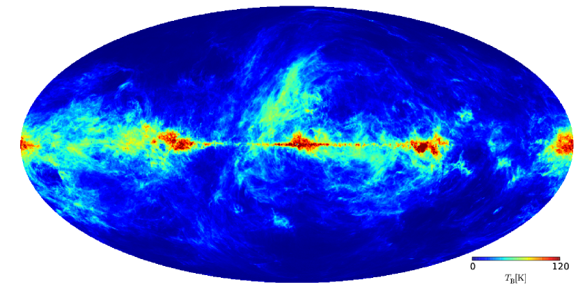
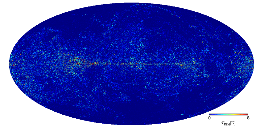
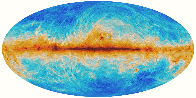
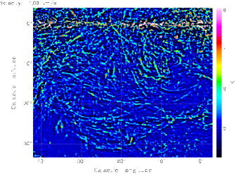
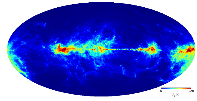
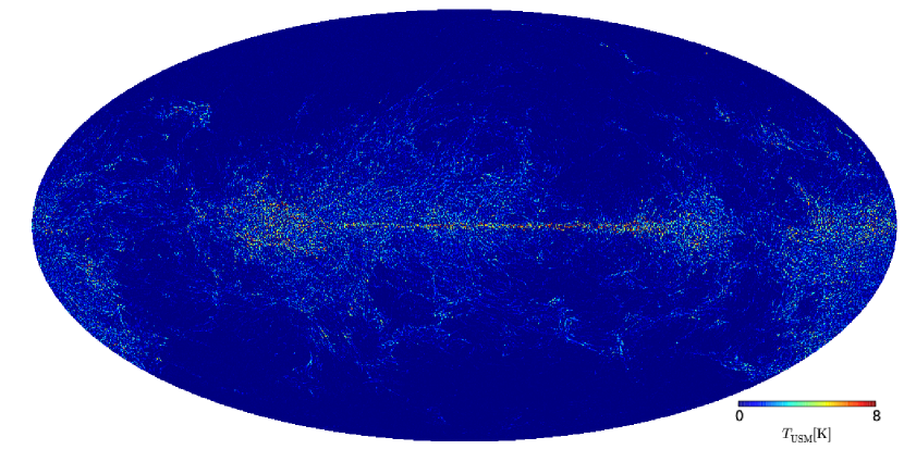
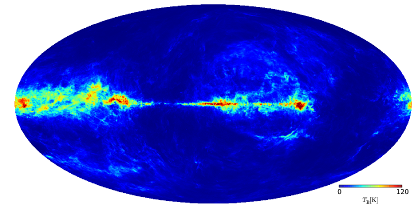
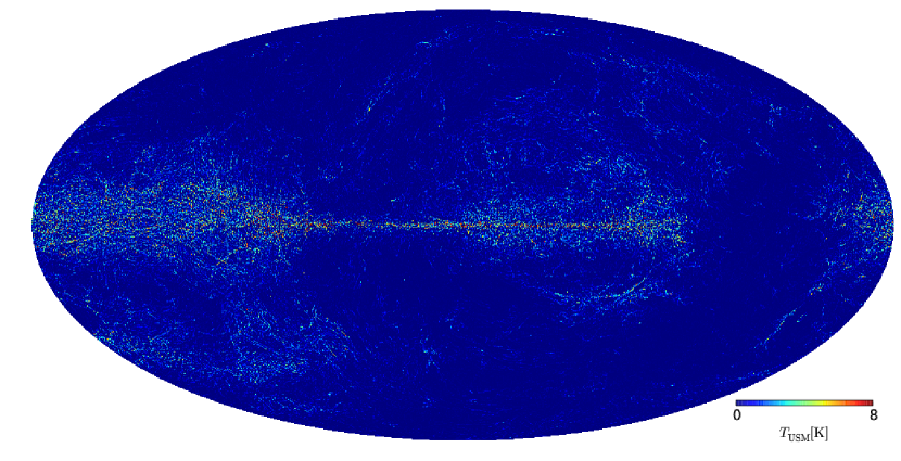
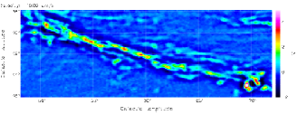
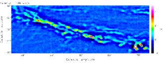
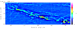
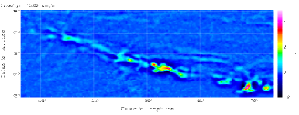
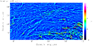
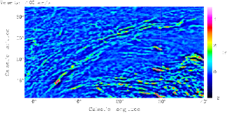
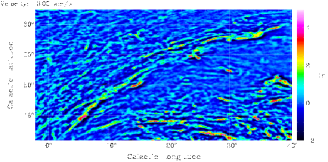
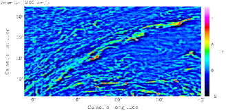
Figures 1, 23, and 24 display three examples. All sky brightness temperature channel maps are displayed in the top panel in Mollweide projection for the radial velocities of km s-1 (Fig. 1), km s-1 (Fig. 23) and +8 km s-1 ( Fig. 24). USM data that emphasize small scale Hi fluctuations are given in the lower panels.
Visual inspection of these channel maps discloses that the USM data in general display only filamentary structures that change significantly in both, position and brightness temperature from channel to channel, implying that the line width of the Hi gas under investigation is comparable to the velocity resolution (channel spacing) of the HI survey data. Such narrow line widths correspond to low kinetic gas temperatures K. Thus, the filaments are physically associated with Hi gas belonging to the CNM (Kalberla & Kerp 2009).
Contrarily, inspecting the observed brightness temperature maps channel by channel shows only minor changes. These maps are dominated by the spatially more extended warm neutral medium (WNM). We interpret the USM features as an indication that the cold filamentary structures are in brightness temperature superimposed to the WNM, perhaps also embedded in it. Whenever we inspect the location of a cold filamentary structures in the USM maps we find corresponding features in the original brightness temperature maps. The opposite search fails in the majority of the cases, even for features that appear visually as unique HI filaments.
Inspecting individual regions at various velocities we often find multiple filaments towards the same area of interest. These filaments reveal for different radial velocities different orientations at the sky. Obviously we are faced with a wealth of cold filaments showing up in the USM maps.
3.1 Deriving global properties of the filamentary HI structures
Given the wealth of filamentary features visible in Fig. 1 (and Figs. 23 and 24 in the Appendix) we obviously need to restrict our analysis to the most prominent ones. We therefore applied the following algorithm to search for major filaments: for each position we check at all velocities km sfor a positive peak in the USM database. In addition to the strength of the USM peak we record its velocity and the corresponding unsmoothed brightness temperature at that velocity. We use the subscript “on” to denote that this parameter is “on source” in position and velocity ; is at the same () position as . We trace for each position the USM features in velocity as long as the intensities remain positive in the USM data base. This allows us to determine the column density and the FWHM velocity width .
From we derive Doppler temperatures (Payne et al. 1980, Eq. 8). This temperature is derived from the observed FWHM line width, corrected for instrumental broadening, and is a measure for an upper limit of the kinetic temperature (Field 1959). Line broadening is caused by a superposition of turbulent motions with (Liszt 2001) and bulk motions along the line of sight. Only in case of a negligible contribution of the turbulent component both temperatures would approach each other, . In Sect. 5.10 we discuss line of sight effects that cause a broadening of observed WNM emission lines. Turbulent line broadening, affecting CNM components, is discussed in Sect. 5.12.
For Hi gas in equilibrium, the kinetic temperature is related to the spin temperature, which is just the excitation temperature of the hyperfine levels evaluated according to the Boltzmann equation (Field 1959). Due to its long life time, the 21-cm transition is usually collisionally excited, and the spin temperature of the gas is a measure for the kinetic temperature. According to Field (1958) the term spin temperature is defined for temperatures derived from absorption lines while kinetic temperatures are determined from the width of Hi lines in thermal motion.

3.2 Selected area studies with the Arecibo telescope
Clark et al. (2014, 2015) have used the (GALFA-Hi) Survey and the first GASS data release (McClure-Griffiths et al. 2009) to search for filamentary Hi features. In both cases the Hi data are not corrected for stray radiation. We note also that GASS data prior to the third data release (Kalberla & Haud 2015) may suffer from residual correlator problems. These can cause artificial linear structures oriented in scanning direction; for details see Kalberla & Haud (2015).
Clark et al. (2014, 2015) used the Rolling Hough Transform (RHT), a machine vision method for parameterizing the coherent linearity of structures in the image plane. The RHT initially was designed for detection of complex patterns in bubble chamber photographs.
The first step in this case is also to apply USM to the image. The image is convolved with a two-dimensional tophat smoothing kernel of a user-defined diameter, DK = 10′ or 15′ for Arecibo, and DK = 53′ for Parkes data. Different in our analysis is that we use a Gaussian smoothing kernel to convolve Effelsberg and Parkes data to an effective resolution of 30′ for both surveys.
After subtracting the smoothed data from the original observations, Clark et al. (2014, 2015) threshold the data at a 70% level to obtain a bit mask. The derived features, called fibers, with a smooth coherent structure and curvature, extend typically across angular scales of a few degrees. In the next step of the analysis the position angle is determined to allow a detailed comparison with the polarization angles of the reflected stellar light and magnetic field directions. Several fibers may exist at individual positions, crossing each other (Figs. 3 and 4 of Clark et al. 2014). To derive a projected RHT field direction, Clark et al. (2015) average Stokes parameters derived at different velocities.
Our focus here is different, we are going to identify the all-sky distribution of the major Hi filaments without modifying the filaments brightness temperature characteristics traced by its curvature or restricting their angular length. For each position we consider only the brightest Hi filament towards each individual line of sight. We do not aim to determine position angles here.
4 All-sky map of Hi filaments
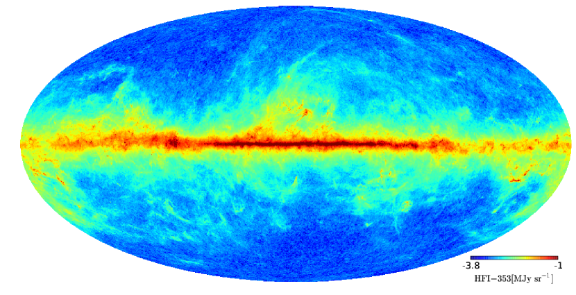
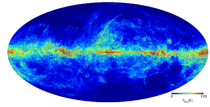
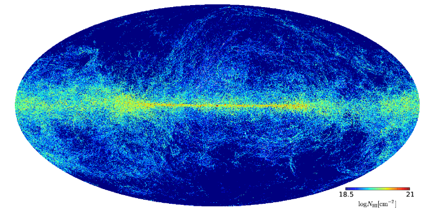
Figure 2 displays the results of our analysis in comparison to dust emission and polarization measured by Planck. The top panel displays the dust emission from the HFI SkyMap at 353 GHz (I_STOKES from the public available HFI_SkyMap_353_2048_R2.00_full.fits in units of MJy sr-1). In the middle panel the brightness temperatures of the major Hi filaments are displayed. This is a presentation of the Hi emission from the gas that hosts the major filaments that we find in the USM analysis. The lower panel of Fig. 2 shows for comparison a composite map of the dust emission as observed by Planck at 353 GHz. Superimposed is a texture derived from the measurements of the orientation of the polarized light emitted by the dust, which in turn indicates the orientation of the magnetic field. The map is from http://www.esa.int/spaceinimages/Images/2015/02/.
Visually the upper two maps show a high degree of correlation between and dust emission except for Hi filaments close to the Galactic plane and in regions with very luminous Hi emission. The lower map displays the global distribution of magnetic fields, in most cases visually aligned by Hi and dust filaments. Many of the fainter Hi filaments show even in details a high degree of correlation between magnetic field lines an the Hi brightness temperature (see Sect. 4.1 in particular Figs. 3 and 4). The general impression is that Hi ridges are in most cases better defined with more detailed substructures than the emission from dust (top). Because of Hi substructures, Hi filaments appear to disclose a higher degree of correlation with the magnetic field lines than the Planck map at the top.
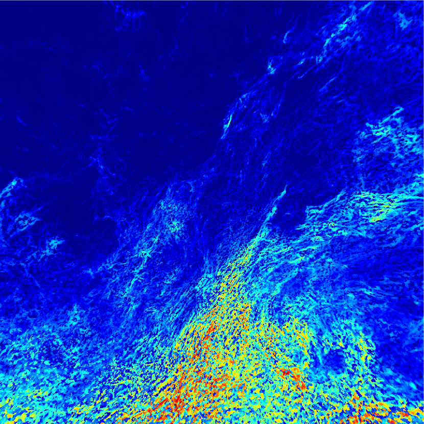
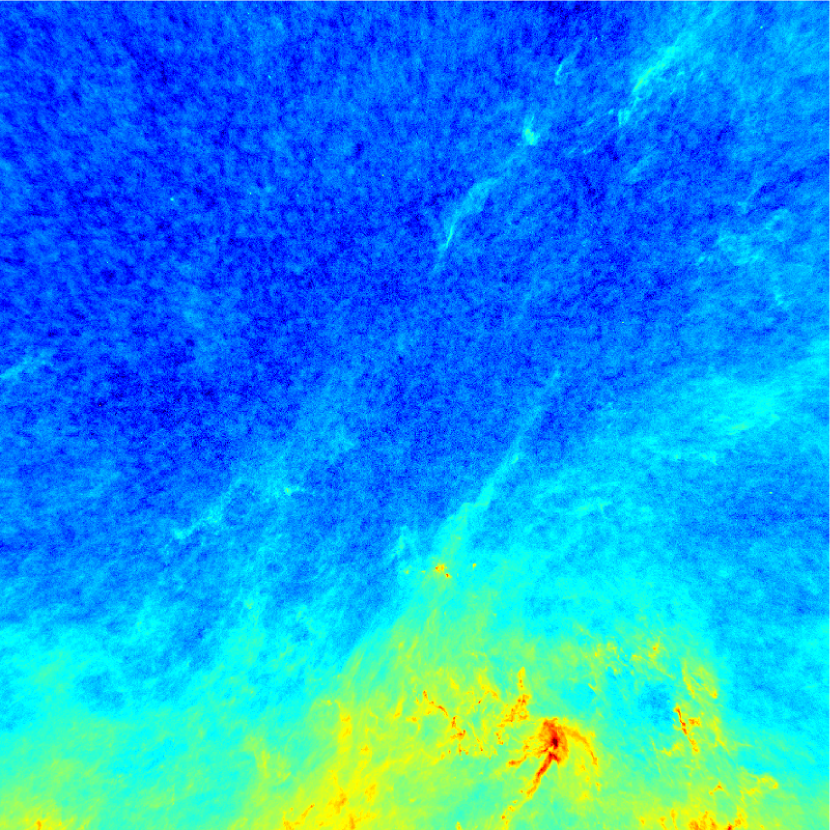
4.1 A detailed comparison between Hi and dust maps
For a more detailed comparison between Hi and dust maps we inspect two interesting regions with prominent filamentary structures. Figs. 3 and 4 give detailed presentations at , and , . It is obvious that the USM Hi data disclose more details at a lower sensitivity limit. Despite the lower angular resolution of the Hi data the Hi reveals much finer details. Next to the major ridges we frequently find striations. The dust intensity map displays a more diffuse distribution. Here, towards the faintest portions of the Planck 353 GHz map we identify intensity fluctuations caused by the cosmic microwave background (Planck Collaboration et al. 2014). Towards the bright far infrared emission the apparent lack of small–scale structure of the Planck data is most likely that the far–infrared emission correlates quantitatively with both, the WNM and CNM. Using USM techniques allows us to determine the velocity where the CNM filament is most prominent. This defines (see Sect. 3.1) and allows to trace the filament, even in case of velocity gradients. Alternatively, an unbound integration over the line of sight would add contributions from unrelated Hi gas. So, the Planck FIR continuum data is indeed limited by the angular resolution of the satellite dishes while the radial velocity information of the single dish Hi surveys allows to differentiate between the WNM and CNM structures.
5 Derived parameters
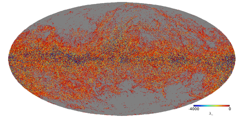
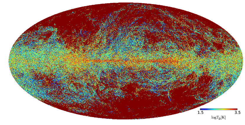
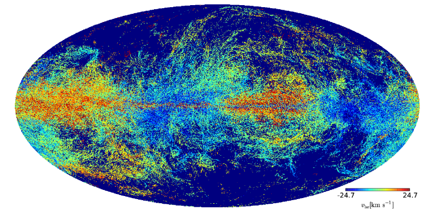
In the following we will parameterize the properties of filamentary structures. Figure 5 and 6 gives an all sky overview and displays in the top panel the principal curvature image of the distribution derived by us. Below we plot column densities for , next the derived Doppler temperatures on logarithmic scale, lg (see Sect. 3.1 for definition of ), and at the bottom the velocity field of the filaments. In all cases we find well defined structures. The purpose of this Fig. is only to highlight global features. All details will be discussed in turn.
5.1 Hessian analysis
Using the USM algorithm, we have derived a map of filamentary structures. Now we discuss whether these structures may also be called filaments in the sense of image analysis.
To classify the curvature of a feature within an intensity map along any direction, the Hessian operator is a useful tool. Schisano et al. (2014) and Planck Collaboration et al. (2016) applied this method recently to astronomical targets. For compatibility we use their notation.
The Hessian matrix is defined as
| (1) |
here x and y refer to true angles in latitude and longitude . The second-order partial derivatives are , , , .
The eigenvalues of H,
| (2) |
are often denoted as principal directions and describe the local curvature of the features; is in direction of least curvature.
We determine the derivatives for (Fig. 2, middle panel) from symmetric differential quotients. Due to the interleaved structure of the HEALPix database it is necessary to interpolate the gridded data in Galactic longitudes, we use a cubic spline interpolation.
Figure 5 (top) displays the principal curvature image, derived from . Images of this kind are often generated for ridge detection in the fields of computer vision and image analysis. Essentially this image reproduces structures seen in the map below or in the middle panel of Fig. 2 and may be compared with Fig. 3 of Planck Collaboration et al. (2016).
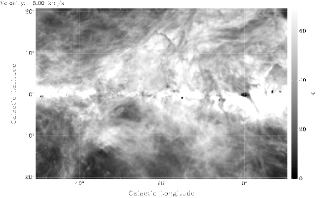

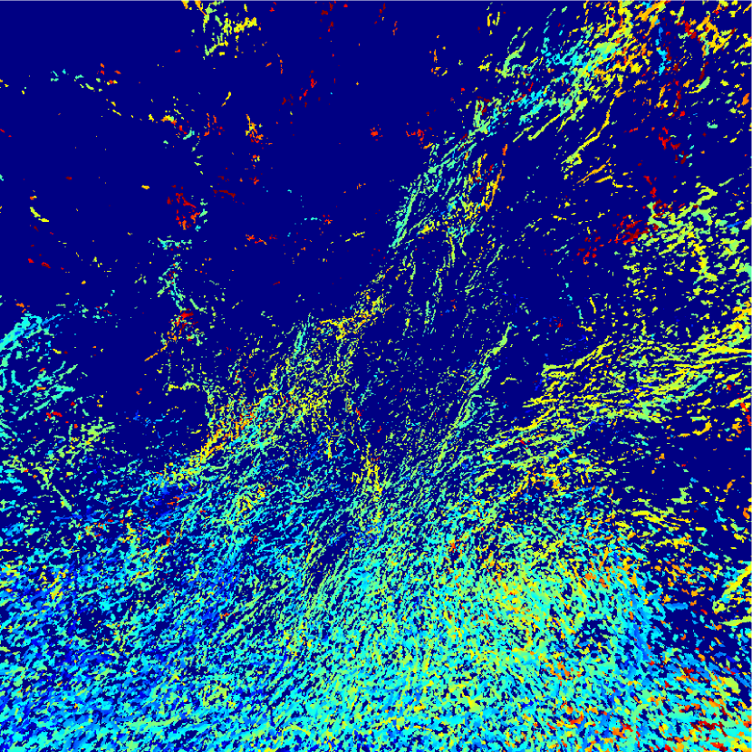
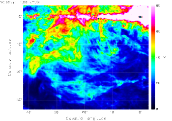
5.2 The Galactic plane
The Hessian analysis is sensitive to point-to-point fluctuations. The noisy blue dotted regions close to the Galactic plane indicate that our basic concept, to define major filaments that are dominating the Hi distribution, approaches its limits towards low Galactic latitudes. This does not imply that there are no well defined filaments in the Galactic plane. The opposite is true, there are too many filaments that overlay each other, causing confusion.
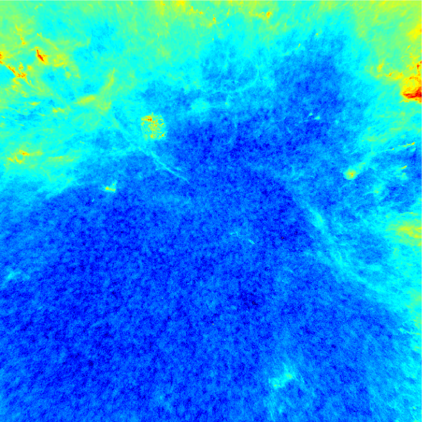
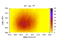
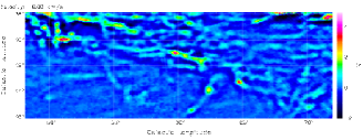
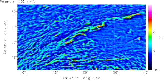
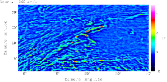
Figure 7 shows as an example an extended region centered at longitude at a velocity of 5 km s-1. To the left we plot the observed brightness temperature, to the right the USM image. This region shows numerous filaments crossing each other. Even within a single spectral channel the confusion is severe. It is worth to note several prominent diagonal features that are due to Hi self-absorption. Close to the Galactic center position is the Riegel-Crutcher Cloud (Riegel & Crutcher 1972; Clark et al. 2014), another structure, almost parallel to the the Riegel-Crutcher Cloud, is at and at . These structures are dark because the Hi is optically thick, leading to self-absorption.
We conclude that the confusion in the principal curvature image is caused by confusion from crowded Hi filaments that are superposing each other. The affected regions in Fig. 5 (top) appear mostly to be spatially correlated to regions with a high polarization angle dispersion function S Planck Collaboration et al. (see 2015a, Fig. 12).
To avoid biases due to confusion by superposition, we focus in the following our analysis to latitudes . The scale height of this gas is limited, hence the observed features are relatively simple with a low probability of confusion. However, for comparison we give also values for the whole sky, to demonstrate that the local interstellar medium at represents well the full sky Hi gas distribution.
5.3 Filament velocities on large scales
The all sky velocity field of the USM filaments is shown in Fig. 6 (bottom). In Fig. 8 some more details on the velocities for the USM filaments displayed in Figs. 3 and 4 are shown. All together we find that filaments share mostly similar velocities but occasionally there are significant gradients in radial velocity perpendicular to or along the filaments. A more detailed discussion on velocity gradients is given in Sect. 5.4. Detailed USM channel maps, showing velocity gradients, are given in the Appendix.
5.4 Filament shapes and orientations
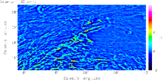
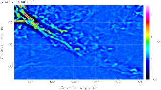
We use Fig. 9 to discuss the observed orientation of filaments with respect to the Galactic plane. Close to the plane it is not easy to identify regions of low confusion levels. This example was chosen to demonstrate that most of the filaments have thin arc-like structures but may run in different directions. Close to the Galactic plane we find filaments without preferred directions. Off the plane, here roughly at , we find filaments that are bent convex, suggestive for an activity of blast waves originating from supernovae in the plane.
5.4.1 Fibers or sheets?
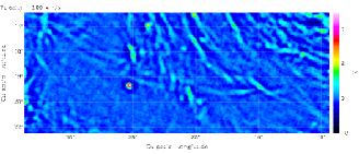
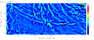
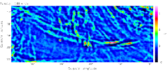
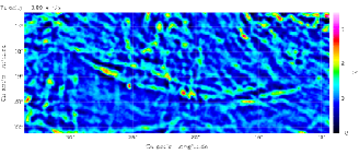
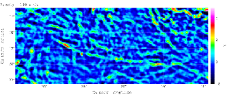
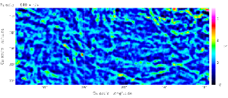
Figure 10 displays details of a pair of filaments located within Fig. 9; both filaments having a length of approximately . Tracing these features shows that they develop subsequently in position-velocity space. The ridges appear to move from channel to channel somewhat less then a beam width, in total 05 over 5 km s-1 before they disintegrate.
Apparent position shifts of Hi structures with channel velocity can be caused by systematic velocity shifts of the gas within a more extended distribution, e.g. as for rotation curves of Galaxies. Significant position changes from one channel to the next, however, can then only be observed for a sufficiently low velocity dispersion of the gas along the line of sight. For a channel spacing around 1.3 km s-1 this implies that the Doppler temperature within the gas layer has to be K. The corresponding FWHM for turbulent motions in velocity is km s-1, only a factor two to five lower than the total correlation width km s-1 that limits the observability of the filaments (see more examples in the appendix). Outside this velocity range the left-over fragments barely resemble a filamentary origin.
Filamentary features of this kind have been described as “morphologically obvious structures” by Heiles & Crutcher (2005); meaning fibers (strings) or edge-on sheets. But how to distinguish between fibers and sheets?
Fibers in the ISM may be caused by sub-Alfvenic anisotropic turbulence (Stone et al. 1998). In simulations such filaments are found to be aligned along the magnetic field lines. That is what we observe but it is unclear how such a model could explain an apparent continuous position shift with velocity.
Hennebelle (2013) studied non-self-gravitating filaments in the ISM. He used MHD simulations to study the formation of clumps in various conditions. It was found that filaments are in general preferentially aligned with the strain due to the stretch induced by turbulence. These filaments survive longer in case of magnetized flows. A strain must affect bulk velocities within filaments. In this case the velocity gradient is along the filament.
According to Heiles & Crutcher (2005) edge-on sheets should be edge-on seen shocks in which the field is parallel to the sheet. Such sheets are observable as filaments when the line of sight becomes nearly parallel to the sheet. Figures 9 and 10 suggest that the filaments are caused by blast waves originating from the Galactic plane. The observed bent convex shapes imply that the filaments are part of a shell. We are observing the shell in almost tangential direction. It is then plausible that we have also some bending in position along the line of sight with an associated continuous change in projected radial velocities, mimicking a position shift perpendicular to the observed filaments. In such a scenario edge-on sheets should be edge-on shocks in which the field is parallel to the sheet, explaining low observed Doppler temperatures.
We use henceforth the notation of Heiles & Crutcher (2005); Heiles & Troland (2005) and assume that the total column density perpendicular to the sheet is . If the normal vector to the sheet is oriented at angle with respect to the line of sight, we observe
| (3) |
In a similar way, if the motion of the sheet is also seen in perpendicular direction, with a velocity , we observe
| (4) |
The observed turbulent velocity dispersion along the line of sight due to projection is given as
| (5) |
(Heiles & Troland 2003b, Eq. 12).
For an angle of , tangential to the sheet or shell, we obtain favorable conditions to observe high column densities . Considering line velocities, we observe velocity crowding (Burton 1971) under the same condition. This additional condition is particularly important in case of low Doppler temperatures.
| (6) |
The observed column densities are strongly velocity dependent and the radial velocities themselves, as bulk velocities within the sheets, depend on projection effects. For nearly tangential viewing, velocity gradients are favorable for an alignment of in filaments.
5.5 Surface filling factor, mass fraction
For a determination of surface filling factor and mass fraction of the USM filaments we use major filaments as defined in Sect. 3.
For the best defined USM filaments at with K, corresponding to a threshold, we find that 30% of the sky is covered by filaments. Lowering the threshold to 0.3 K, the coverage increases to 60%. Repeating the analysis with a 0.1 K constraint and including in this case also the Galactic plane we estimate that 95% of the sky is occupied. Filaments are ubiquitous.
The relation between and for all positions is displayed in Fig. 11. We find a large scatter, most of the filaments are found in regions with low brightness temperatures , correspondingly the values are low.
We estimate the mass fraction of the Hi gas in major filaments from , integrating over all positions with . For a thresholded K we find and for threshold of 0.3 K we get . Our derivation of the mass fraction assumes that the gas in filaments as well as the surrounding warm medium is optically thin, for detailed discussion see Sect. 5.9. The filling factor , derived so far, considers only major filaments. There may be more than a single filament along the line of sight, we need accordingly to determine , integrating unconstrained across all significant filaments along the line of sight. This way we obtain a total fraction .
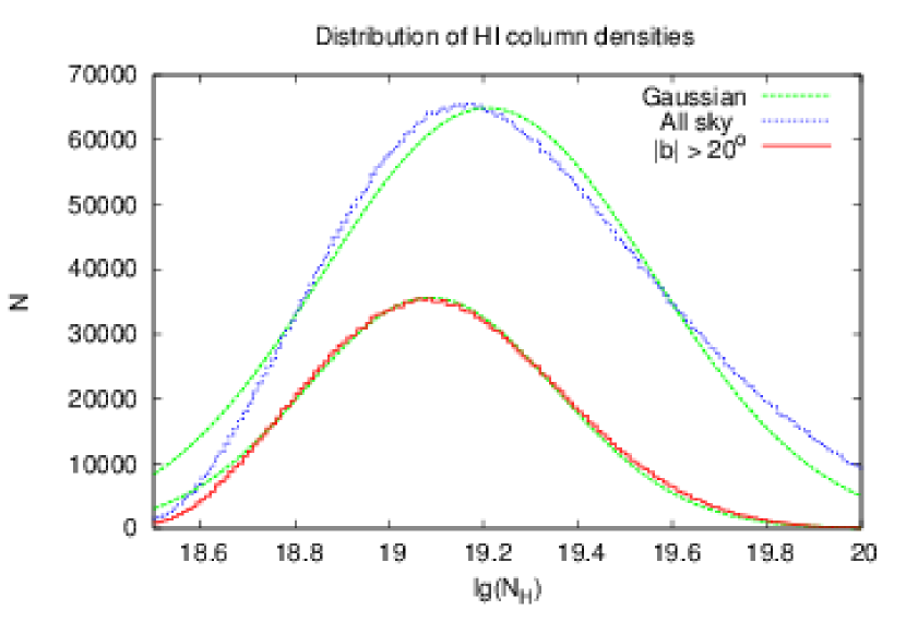
5.6 Column densities
Next we derive column densities for the Hi gas in filaments, assuming that the gas is optically thin. Possible biases due to optical depth effects are discussed in Sect. 5.9. We use a threshold of 1 K.
Figure 12 displays the probability density distribution (PDF) for the filament column densities. This plot shows a log-normal distribution with a well defined maximum at for the gas with with a dispersion . The median111For a turbulent medium the characterisic PDFs are log-normal (Vazquez-Semadeni 1994) as a result of the central limit theorem applied to self-similar random multiplicative perturbations. The geometric mean of a log-normal distribution is equal to its median. Reading off peak values from plots of PDFs published on a linear scale leads to biased results. column density is . Including the Galactic plane leads to an increase of the column densities, also the peak shifts somewhat. This shift implies that confusion, discussed in Sect. 5.2, tends to increase the apparent column densities of the filaments. This distribution deviates from a simple log-normal PDF.
Clark et al. (2014), in their analysis of a region that covers about 1300 degr2, considered only a single characteristic fiber within this field. They mention a typical column density , only 25% different from our result.
5.7 Volume densities from distance estimates
A standard assumption is that column densities around cm-2 are optically thin, but optical depth effects may be significant (see Sect. 5.9), causing volume density biases. Another problem is beam dilution. Assuming a distance of 100 pc, the median distance to the wall of the local cavity (Lallement et al. 2014, from color excess measurements), the FWHM of the telescopes corresponds to 0.3 pc and is therefore a limit to the spatial resolution.
Hi ridges appear to move from channel to channel somewhat less than a beam width (Sect. 5.4.1). This implies that within the telescope beam the line of sight velocities of the Hi cannot differ much more than the channel width. For an Hi sheet with isotropic turbulence the velocity dispersion across the beam has to be similar to the dispersion in perpendicular direction, along the line of sight. In turn, since in turbulent media scale length and velocities are related to each other, the depth along the line of sight should be comparable to the one in perpendicular direction. In presence of velocity gradients across the beam the derived depth is an upper limit only.
For an estimate of the volume density we assume hence a filament with a thickness of 0.3 pc. For a typical column density cm-2 we obtain a volume density of cm-3. Clark et al. (2014) derive a similar value from Arecibo survey data but later in Sect. 5.12 we will argue for a thickness of pc and a density cm-3.
Different environmental conditions were assumed by Planck Collaboration et al. (2016) for the gas associated with dust. Based on a local scale height of 100 pc they assume an average filament distance of 430 pc. This corresponds to a thickness of about 1 pc, adopting spherical symmetry and an angular extent of the filament equal to the size of the antenna beam. We obtain in this case a volume density of 4 cm-3. Assuming standard gas-to-dust conversion, Planck Collaboration et al. (2016) derive an average Hi volume density of 300 cm-3. At the first glance there appears to be a huge discrepancy between both values. But we need to consider that the Planck data trace all gaseous species while the USM data selects the CNM. Applying the previously determined factor we obtain a volume density of 27 cm-3, only a factor of two different from our first estimate which was based on a filament distance of 100 pc.
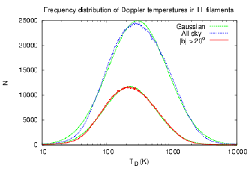
5.8 Doppler temperatures
It is feasible to estimate roughly the temperatures of the Hi gas from the distribution. From the close agreement between dust emission and filaments in (top and middle panel of Fig 2) one may suspect a physical association between the filaments which implies that these Hi features must be cold.
From the line-widths of USM filaments we determine Doppler temperatures. In Fig. 13 we display the distribution in a histogram. Restricting our analysis to (red curve), we obtain a well defined log-normal PDF. The median is K; from the Gaussian fit we obtain K, corresponding to a FWHM line width of 3.2 km s-1. Including the Galactic plane leads to somewhat higher Doppler temperatures, with a peak at K. Apparently, even in case of confusion there are only slight biases towards higher Doppler temperatures. A previous Gaussian decomposition of the LAB survey by Haud & Kalberla (2007) yield for the narrowest components in a log-normal distribution with K at a FWHM of km s-1. For a distribution affected by radial velocity gradients across the beam, the smoothing will increase the line widths and the Doppler temperatures in case of a larger telescope beam.
The log-normal Doppler temperature distribution is, similar to the column density PDF (Fig. 12), approximated surprisingly well by a single Gaussian, we observe a remarkable clean single-phase relation. Also in case of Doppler temperatures we obtain an excellent agreement between our results and those of Clark et al. (2014) who derive K. According to the estimates above, the thermodynamic pressure of the filaments is K cm-3, in reasonable agreement with the standard pressure found in the ISM at the solar circle K cm-3 (Wolfire et al. 2003). Clark et al. (2014) derive a pressure of K cm-3.

5.9 Optical depth effects and self-absorption
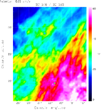
USM column and volume densities, discussed in Sects. 5.6 and 5.7 may be affected significantly by optical depth effects. Having merely Hi emission data, we neither can determine optical depth nor spin temperatures for the filaments. However at a few positions, absorption data are available from Heiles & Troland (2003a). Here we will compare their data (column densities , optical depths , spin temperatures , and upper limits to kinetic temperatures ) with our results (Doppler temperatures and column densities ). Note that Heiles & Troland (2003b) use in place of . Our estimates are derived at positions close to the continuum sources along the filaments. We study accordingly two fields with strong background sources.
Covered by the area of interest displayed in Fig. 14 we have 3C348 and 3C353 and Hi filaments are crossing these sources.
For 3C348 we estimate close to the source at km s-1 along the filament a Doppler temperature of K and a column density cm-2. From Arecibo data Heiles & Troland (2003a) obtain an optical depth of and temperatures K and K. We miss almost a factor of 8 in the measured column densities.
For 3C353 we estimate at km s-1 a Doppler temperature of K. From Arecibo data Heiles & Troland (2003a) determine K but a spin temperature as low as K. The optical depth is high. Correspondingly, the column density is cm-2, but we derive only cm-2.
Common for both is that the CNM gas shows up with spin temperatures around 30 K. Both are located in regions with a similar background temperature, K for 3C348, and K for 3C353. Some self-absorption might be present (Gibson et al. 2000). In absence of a continuum background source the difference in brightness temperature due to the CNM cloud is given by
| (7) |
Here is the spin temperature and the brightness of the WNM background. is the unknown fraction of the gas that is beyond the CNM filament. For self-absorption becomes important, thus the HI emission of the filament may be attenuated strongly. Thus we expect that for K self-absorption may be recognizable. 20% of the CNM filaments at latitudes are considered to be affected. However, checking these data we find no indications for obvious self-absorption, rather the average CNM column densities increase by 23%. This implies, that in regions with luminous WNM emission also the CNM column densities tend to be higher. Hence, at latitudes no indications for obvious self-absorption effects are evident from our analyses, opposite to the examples at low latitudes as shown in Fig. 7. Checking whether depends on we find no significant trends with . We also applied an optical depth correction for the column densities according to Martin et al. (2015, Eq. 8). Testing for spin temperatures ranging between 20 and 80 K, again no significant effects are found for the distribution plotted in Fig.12.
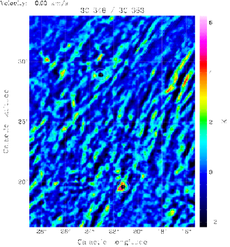
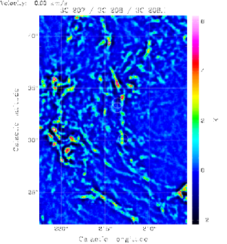
In Fig. 15 we have 3 continuum sources, 3C207, 3C208, and 3C208.1. There are no clear filaments but a number of Hi fragments, perhaps originating from a disintegrated filament. At a velocity of km s-1 the Hi in front of 3C207 Heiles & Troland (2003a) determine an optical depth and a spin temperature of K, the Arecibo limit to the kinetic temperature is K. We determine a K and a column density cm-2, compared to an Arecibo column density of cm-2.
The Hi in front of 3C208, and 3C208.1 has at a velocity of km s-1 optical depths below . But for 3C208 at km s-1 our Doppler temperature K compares to an Arecibo spin temperature of K, the column densities are within an uncertainty of 40% comparable. For 3C208.1 at km s-1 we have , compared to K and our column density is 40% higher than that from Arecibo.
Self-absorption for the 3C207/208 field are considered to be insignificant because the low WNM temperatures close to the continuum sources are only K.
We conclude that Doppler temperatures and column densities for the filaments, derived by us, are quite uncertain but roughly consistent with parameters from Heiles & Troland (2003a) as long as the optical depth is low. We cannot measure the optical depth and for values we may seriously underestimate the column densities.
The question arises what fraction of the filamentary Hi gas at latitudes is optically thick. In our examples we considered two cases with quite different morphologies, regular parallel filaments and less ordered fragments. In both cases the dust emission from the HFI Sky Map at 353 GHz is rather low. Is there, concerning optical depth effects, a systematical difference between both cases, regular or broken filaments?
5.10 Filaments within a warm environment
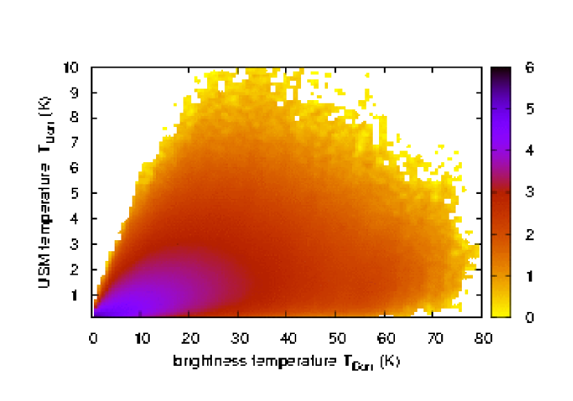
Figures 1, 23, and 24 suggests that the filaments with low intensities are embedded in a warmer environment that dominates the observed distribution. We use an all-sky Gaussian decomposition (Haud 2000; Haud & Kalberla 2007; Kalberla & Haud 2015) of the observed brightness temperature distribution to search for this surrounding gas. At each position for we select components with center velocities , where is the dispersion corresponding to FWHM line width . Note that this condition is very stringent concerning the center velocities. Narrow ( km s-1) and insignificant low intensity components ( K) are disregarded. We use the best fitting component with the lowest velocity dispersion and exclude this way broad features that might be unrelated to the filaments. Using (Sect. 3.1) we convert line widths to Doppler temperatures.
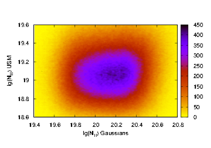
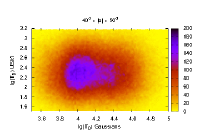
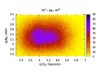
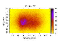
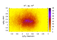
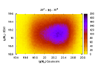
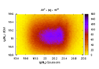
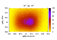
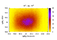
Figure 16 shows the 2-D density distribution for Doppler temperatures within Hi filaments and the surrounding WNM gas. The horizontal spread corresponds to the range of the WNM Doppler temperatures lg(), while vertically lg() for the USM filaments is displayed. This plot is consistent with a two-phase distribution, cold filaments are embedded within a warm environment with a median K.

We also determined the two-phase distribution of column densities. Figure 17 shows that the filaments with typical column densities cm-2 are embedded in a WNM with typical column densities of cm-2. From the column densities we derive consistent with Sect. 5.5 a mass fraction of , yielding including selection effects for multiple filaments along the line of sight as discussed in Sect. 5.5.
5.10.1 Latitude dependence
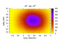
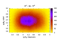
Next we study whether derived Doppler temperatures may depend on Galactic latitude. In Fig. 18 we display the 2-D density distributions of Doppler temperatures for several latitude ranges. We find no significant changes in the distribution of the Doppler temperatures for the filaments, the peak at lg() , corresponding to K, remains almost constant. However the distribution for the warm envelopes shows some variations between , corresponding to K.
Figure 19 displays latitude dependent 2-D density distributions of the column densities. Filament column densities change only marginally, with a peak from cm-2 at low latitudes to cm-2 at high latitudes. For the WNM envelopes the dependency is much more significant, .
The Hi vertical distribution in the solar neighbourhood can be described as a layer with approximately constant scale height (Kerr 1969). The path along the line of sight through this layer follows . We obtain from this relation for the WNM a factor of 2.4 in column density while we observe an increase by a factor of 2.5, consistent with the hypothesis that the WNM distribution can be approximated by an extended layer.
The filaments do not show any significant latitude dependence, neither in Doppler temperatures, nor in column densities. We conclude that these parameters do not depend on latitude and are unaffected by other line-of-sight effects.

5.11 Two-phase stability
Models of the ISM assume that on average the WNM and the CNM are in pressure equilibrium. Our current knowledge about heating and cooling in the Solar vicinity is based on a fiducial column density of cm-2 at the WNM/CNM boundary. This implies a local pressure K cm-3 (Wolfire et al. 2003, Sect. 6.1). Accordingly the CNM can exist for thermal temperatures K. The allowed temperature range for the NM is K. Hi gas at temperatures K is thermally unstable.
This model is in conflict with our determination of a WNM column density of cm-2 in Sects. 5.6 and 5.10.1. Phase diagrams, showing the dependence of and hydrogen nucleus density for different values of the WNM column density, are given in Fig. 9 of Wolfire et al. (2003). According to Table 3 of the same paper the column densities determined here imply an average pressure at the solar circle of K cm-3. Stability for CNM clouds is thus expected at a somewhat higher temperature range K. The low pressure K cm-3 is however in conflict with a recent determination of the local thermal pressure of K cm-3 by Jenkins & Tripp (2011). According to a private communication by Mark Wolfire the theory of the two-phase ISM demands a revision and the WNM column density of cm-2 appears to be today consistent with a pressure around K cm-3.
To finally proof stability it would be necessary to determine kinetic temperatures of the CNM filaments under investigation. From our observations we can only determine Doppler temperatures that are affected by turbulent motions of the gas. However, it is feasible to constrain them by some ensemble properties.
Turbulent motions in the CNM can be characterized by the turbulent Mach number
| (8) |
(Heiles & Troland 2003b, Sect. 6.2.4). CNM clouds tend to be strongly supersonic and high Mach numbers are common (Heiles & Troland 2003b, Fig. 12).
The all-sky maps, shown in Sect. 4, imply that CNM filaments are sheets, aligned to the magnetic fields. For such an alignment Heiles & Troland (2005) determine from the Millennium Arecibo 21-cm absorption-line survey a median magnetic field strength of G. They find that turbulence and magnetism are in approximate equipartition with a characteristic turbulent Mach number at a median thermal CNM temperature of 50 K.
Our data are consistent with this proposal; for the median Doppler temperature K of the filaments corresponds to a thermal temperature of 52 K. The upper limit for a stable CNM with a temperature of 258 K corresponds then to a Doppler temperature of 1100 K; Fig. 13 shows only few components in excess of that limit.
Heiles & Troland (2005) did not consider a latitude dependence of the derived parameters. Using data from the Arecibo Millennium survey (Heiles & Troland 2003a), restricting their sources to latitudes and spin temperatures to K, we obtain a median Mach number . In this case we derive an upper limit of K for the stable CNM phase and already 5.5 % of the components plotted in Fig. 13 may be unstable. For , discussed in Sect. 5.12, this fraction increases to 6.6%.
We conclude that in presence of a magnetic field the CNM population derived by us can be stable against thermal instabilities. Without magnetic field support some fraction of the filaments would probably be unstable. According to Heiles & Troland (2005) the magnetic pressure is , significantly higher than the thermal pressure. In Sect. 5.12 we will show that the thickness of the CNM filaments is dictated by the magnetic field, leading to a median CNM volume density of .
For the WNM at we find, if we disregard turbulence, that only 3% of the components have a Doppler temperature below 5040 K, the lower limit required for stability. But adopting also for the WNM a correction for turbulent motions, with a typical Mach number of , we denote that almost 60% of the components would be below the temperature limit required for stability. This exercise implies that the amount of unstable WNM gas depends critically on the turbulent Mach number which is today only poorly known.
The median K (Sect. 5.10 and Fig. 15) in combination with the WNM gas temperature of K (Wolfire et al. 2003) yields a WNM Mach number of . In this case 27% of the WNM gas would be unstable. Heiles & Troland (2003b) derived a lower limit of 48% for the CNM-associated WNM gas in the thermally unstable region but the lower limit of 28% to 30%, determined by Roy et al. (2013); Roy (2015), is in better agreement with our result.
5.12 Magnetic pressure confinement for the CNM
To probe the role of magnetic field confinement for the CNM filaments, we evaluate in the following the relevant physical parameters. We assume a homogeneous sheet with a volume density , hosting the turbulent CNM gas with a Doppler temperature . Consequently the gaseous pressure is . For a thickness along the line of sight we observe a column density , hence . Assuming now that the shape of the Hi sheet is entirely confined by a magnetic field with a magnetic pressure , we obtain for pressure balance the condition
| (9) |
According to Heiles & Troland (2005, Sect. 3.1.3 & 9), internal turbulent motions have in this case to be two-dimensional, restricted to directions perpendicular to the mean magnetic field. For a turbulent Mach number and an Alfvèn velocity km s-1, turbulent motions along the magnetic field lines are thought to cause shock waves, and such oscillations are strongly damped. Gravitational instabilities are not expected for the CNM (Heiles & Troland 2005, Sect. 7.2).
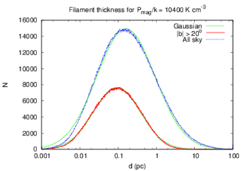
From our observations we deduce and . With a magnetic pressure K cm-3 from Heiles & Troland (2005), we can derive . Figure 20 shows the PDF for the derived filament depths . We obtain a well-defined log-normal distribution, for with a peak at pc, the median filament thickness is pc. The all sky distribution has a maximum at pc with a median pc.
We obtain here only 1/3 of the upper limit for derived in Sect. 5.7 from estimates based on the median distance to the wall of the local cavity (Lallement et al. 2014). Consistently, for a median K we get also a characteristic volume density that is three times as large as determined previously. The single dish telescopes used are limited in angular resolution to structures of 0.3 pc size at 100 pc distance. Systematic velocity gradients below this angular resolution limit can be traced because of the low gas temperatures. Velocity gradients are observed frequently on larger scales perpendicular to the main axis of the filament (see e.g. Figs. 10, 25, and 26) and sometimes along the filament (Fig. 27). Note, the determination of the filament thickness according to Eq. 9 is not a function of distance or geometry and thus independent on the angular resolution of the HI data analyzed. The derived thickness pc (from Eq. 9) corresponds only to 1/3 of our spatial resolution, so it is a lower limit for the filament thickness with an uncertainty of about 30% due to uncertainties of the average magnetic field strength (Heiles & Troland 2005).
The derived median filament thickness of 0.09 pc depends stongly on the hypothesis of magnetic pressure confinement and it may be questionable whether such a case applies. The Arecibo telescope has a far better spatial resolution but Clark et al. (2014, Sect. 8.1) claim that the filaments are “largely unresolved and therefore correspond to pc” at a distance of 100 pc. Within the uncertainties this estimate is compatible with our result and strengthens the case for a magnetic pressure confinement. The Square Kilometre Array (SKA) is needed to resolve the detailed spatial structure of the filaments.
In case of a thermal equilibrium the median volume density of yields at a pressure of a gas temperature of K. The corresponding median Mach number is . Using data from the Arecibo Millennium survey (Heiles & Troland 2003a), restricting their sources to latitudes and spin temperatures to K, we obtain medians and K. Both values are also within the uncertainties consistent with our results. The derived gas parameters, adopting magnetic pressure confinement, describe a stable CNM gas phase and fit best to the model assumptions (Wolfire et al. 2003, Sect. 6.1) with an average temperature K and density .
Confinement of gaseous phases is not limited to the atomic phase only, it is applicable also to molecular gas. In this respect latest Herschel measurements (André et al. 2014) are of particular interest. Consistent with the values derived for the atomic phase André et al. (2014) find filaments in dense star forming region with linear extents of pc. Moreover, Federrath (2016) concludes from high-resolution MHD simulations that follow the evolution of molecular clouds and the formation of filaments and stars, that there is a remarkably universal filament width of 0.10 pc which is independent of the star formation history of the clouds.
Because of saturation effects, Hi filaments in regions with molecular gas are not well defined but we find a general trend that filaments in such regions are more extended. This is expected since molecular gas condensations are mostly located interior to Hi filaments. Close to the Galactic plane, for , we find pc but it is unclear, how far this result is biased by confusion.
5.13 Global velocity distribution of the filaments
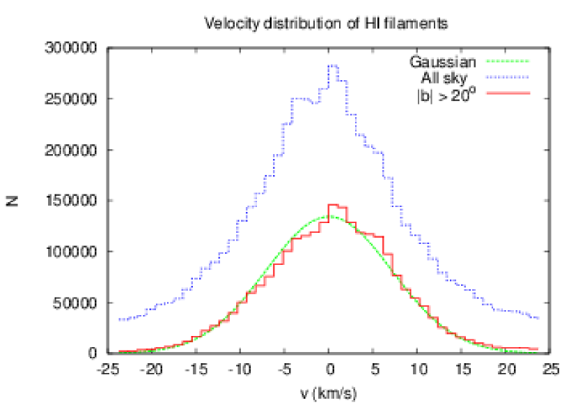
The histogram in Fig. 21 displays the global distribution of center velocities for all USM filaments. The red curve gives the distribution for latitudes and can be approximated by a Gaussian with a FWHM width of km s-1, centered at km s-1.
The Gaussian shape of the velocity distribution is remarkable since in theory there is no consensus that the probability density distribution of the velocity has to be Gaussian (Elmegreen & Scalo 2004). According to the central limit theorem the arithmetic mean of a sufficiently large number of independent random variables, each with a well-defined mean and well-defined variance, will be approximately normally distributed. Around the Sun we have a random distribution of filaments, triggered by random events. Apparently, the presence of distinct filaments, each with well defined velocity centroids, does not preclude that we have in total a random distribution. The channel maps displayed in Figs. 1, 23, and 24 are chosen to be at the velocities of the peak and half width points, hence they are characteristic for local filaments.
From the Gaussian shape of the velocity distribution in Fig. 21 we infer that our sample of CNM clouds, which is complete for , represents a well defined and unbiased ensemble of objects in turbulent motion. The width of the velocity distribution is then a measure of the kinetic energy. We derive a formal turbulent temperature of 6500 K. This value is low in comparison to the median Doppler temperature of the WNM gas, K (Sect. 5.10) but fits to the allowed thermal temperature range of K for the WNM (Wolfire et al. 2003). Our result is consistent with numerical simulations of Saury et al. (2014) on the structure of the thermally bistable and turbulent atomic gas in the local interstellar medium. They found that “the structure of the CNM and WNM are tightly interwoven: the two media share the same velocity fields and the CNM cloud-cloud velocity dispersion is close to the WNM sound speed”.
Including the Galactic plane in our analysis we find significantly more filaments at high radial velocities (blue curve in Fig. 21). This is consistent with Fig. 5 (botom) that shows at low latitudes some signs of Galactic rotation. Once more we find indications that our definition of major local filaments appears to be ill-defined at low Galactic latitudes, the ensemble properties are significantly affected by non-local gas.
5.14 Kinetic energy distribution
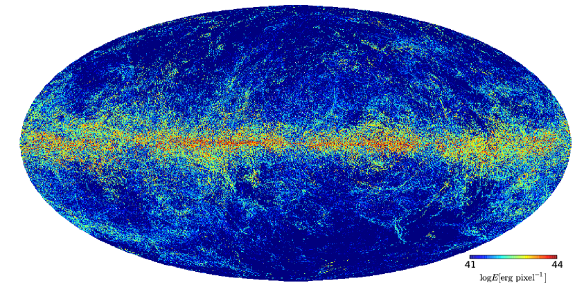
Filaments, if caused by blast waves originating from supernovae, are thought to resemble the dynamical properties of their origin. We expect that these sources are located around us close to the Galactic plane. Filaments should tell us then about the mechanical energy that was injected into the ISM. For observed radial velocities of filaments and USM column densities we calculate an all sky map of the kinetic energy distribution. Here we assume for all Hi filaments a distance of pc. We apply a brightness temperature threshold 0.3 K.
For an individual pixel in the nside = 1024 map we obtain a kinetic energy
| (10) |
Figure 22 shows this estimate for the energy distribution in filaments, the look up table is logarithmic in ergs/pixel. The total energy, integrating over the sphere, is ergs. For low latitudes, , we find high energies but this is subject to confusion, also most probably significantly affected by non-local sources. The distribution at high latitudes deviates significantly from Figs. 2 and 5. The reason is that the kinetic energy in Fig. 22 depends on while Figs. 2 and 5 are not weighted by radial velocity.
Our estimate for the energy distribution suffers certainly from unknown distances. But we do not see obvious structures that show signatures of the walls from the local cavity (Lallement et al. 2014). The large scale filaments at intermediate negative latitudes in the anti-center are probably at larger distances (Lallement et al. 2014, Figs. 11 & 12).
6 Summary and conclusions
We explored the data of the first Galactic EBHIS data release and merged them with the GASS III survey. Using USM methods we extracted the Hi distribution on scales of to and derived all sky maps of unprecedented quality. Filamentary Hi gas structures are visible nearly everywhere. Analyzing the most prominent structures (major filaments) we demonstrate that these filaments show a good agreement with the polarized Galactic dust emission observed by Planck.
All the sky is full of filaments but restricting our analysis to the most prominent local structures for USM temperatures K, corresponding to a threshold, we obtain a distribution that is in surprisingly close agreement with the dust emission observed by Planck at 353 GHz (Figs. 2, 5, and 6). Individual filaments can be traced in detail, but in the Galactic plane we find confusion. We draw the conclusions of our analysis for latitudes but demonstrate also that in the Galactic plane most of the derived parameters are not seriously affected by confusion.
We do not attempt to correlate Hi filaments with Planck polarization data at 353 GHz. From a direct comparison between Hi and Planck 353 GHz maps it is obvious that we trace similar features (our Figs. 2 to 5). Also the Hessian analysis gives identical results (Sect. 5.1, see also Fig. 3 of Planck Collaboration et al. (2016)). From Planck data it is evident that for low Hi column densities cm-2 filaments lie along magnetic field lines (Planck Collaboration et al. 2015a; Planck Collaboration et al. 2015b, 2016). Such a correlation was also shown by Clark et al. (2014, 2015) who used Arecibo data. So we can well assume that Hi filaments studied by us are associated with magnetic fields.
The full-sky single dish HI surveys allow for the first time to establish a complete census of the local CNM. All high Galactic latitude filaments, but also the the bulk of the gas located close to the Galactic plane, share a common set of physical parameters describing the ISM conditions. The gas is characterized as a CNM with a median Doppler temperature of K; it has column densities around cm-2. The probability density distributions are very well approximated by a log normal one and independent of position. The maxima of the PDFs agree with the medians. Filaments appear isolated but may be accompanied by other filamentary structures, similar to striations, in the vicinity.
The widhts of the CNM filaments are unresolved by our telescopes. Adopting a typical filament distance of 100 pc to the wall of the local cavity (Lallement et al. 2014) we derive for the CNM sheets a thickness of pc and correspondingly a volume density of cm-3 (Sect. 5.7). Clark et al. (2014) claim that filamentary structures, observed by them, are unresolved with the Arecibo telescope. This implies a sheets thickness of pc. Considering in addition pressure confinement from a magnetic field of G (Heiles & Troland 2005) we derive a distance independent lower limit of pc for the median sheet thickness, consistent with the Arecibo results. Such a sheet depth implies an upper limit for the median volume density of cm-3. Our analysis discloses that the CNM is organized in cold filaments that are aligned with, and dominated by, magnetic fields.
These filaments are embedded in a more extended warm gas phase with column densities that are an order of magnitude higher (Sect. 5.10). From our data alone it is difficult to comment on the stability of the two phases. In Sect. 5.11 we consider the CNM and conclude that for a turbulent Mach number of at least 93.4 % of the CNM filaments should populate the stable part of the phase diagram (Wolfire et al. 2003). In case of magnetic pressure confinement (Sect. 5.12) all CNM filaments can be safely considered to be stable. The stability issue is less clear for the WNM. We argue in Sect. 5.11 that 30% of the WNM that is in contact with the CNM filaments may be unstable.
Our analysis contains a few parameters affected by systematic biases. From emission data alone it is not feasible to determine optical depth effects. A rough comparison with Arecibo absorption observations (Sect. 5.9, data from Heiles & Troland (2003b)) indicates, within the accuracy of both analyses, consistent results except for optical depths . For optically thick gas we seriously underestimate the column densities, hence also derived volume densities are biased. We determine for the optical thin filaments a mass fraction . This is low in comparison to the canonical value of 0.40 (Heiles & Troland 2003b) but we estimate that if only about 10% of the observed filaments are optically thick the apparent discrepancy may cease.
The velocity structure of the local gas filaments is remarkable. We find for the whole sample a Gaussian velocity distribution, centered at km s-1, with a FWHM spread of km s-1. On large scales filaments have frequently companion features at similar velocities. We find some USM structures that can not be described as obvious filaments. Partly such fragments look like disintegrated features from filaments, partly they may be caused by projection effects, as a result of apparently crossing filaments. In fact, any geometry is possible; i.e. the spider (Planck Collaboration et al. 2011, Fig. 9 & 13) is caused by several crossing filaments, easily traceable in the USM channel maps.
Using USM with a fixed Gaussian smoothing kernel (effective FWHM of ) may cause biases in the analysis because spatial frequencies corresponding to the FWHM beam sizes of the Parkes and Effelsberg telescopes are preferred. All derived parameters were compared with those by Clark et al. (2014, 2015) who used predominantly Arecibo data for their analysis. In all cases we found excellent agreement. The methods that have been used by this team are very different from ours. This implies that neither our analysis nor that of Clark et al. (2014, 2015) are strongly affected by systematical effects. Also there is no recognizable dependence on telescope size or spatial resolution. Arecibo is far ahead with respect to the beam width and velocity resolution but unfortunately restricted with respect to the observable portion of the sky.
The most striking result from our investigation is the large number of extended cold coherent filamentary structures that we observe. A number of these features reach angular scales of , implying a total length of pc at an assumed distance of 100 pc. CNM sheets of this kind were previously observed and discussed by Heiles & Troland (2003b). A median sheet width of 0.09 pc implies length-to-thickness aspect ratios up to 400 or more. For comparison, the edge-on aspect ratio of a CD is 100. The two-phase model is based on observational evidence that the CNM is embedded in the WNM, giving rise to the so called “raisin pudding” model (Field et al. 1969). Our data imply that the CNM clouds are very different from standard clouds (Spitzer 1968; McKee & Ostriker 1977) or “raisins” (Clark 1964). What we observe are rather “steamrollered raisins”, flatter than a CD, and warped by a turbulent ISM. The magnetic field appears to play a major role in this process.
Initially we intended to explore the quality of an all-sky survey. The combined EBHIS/GASS III survey shows an excellent performance, acting well as a pathfinder for future SKA observation.
References
- André et al. (2014) André, P., Di Francesco, J., Ward-Thompson, D., et al. 2014, Protostars and Planets VI, 27
- Bajaja et al. (2005) Bajaja, E., Arnal, E. M., Larrarte, J. J., et al. 2005, A&A, 440, 767
- Boulanger et al. (1996) Boulanger, F., Abergel, A., Bernard, J.-P., et al. 1996, A&A, 312, 256
- Burton (1971) Burton, W. B. 1971, A&A, 10, 76
- Clark (1964) Clark, B. G. 1964, Ph.D. Thesis, California Institute of Technology
- Clark et al. (2015) Clark, S. E., Hill, J. C., Peek, J. E. G., Putman, M. E., & Babler, B. L. 2015, Physical Review Letters, 115, 241302
- Clark et al. (2014) Clark, S. E., Peek, J. E. G., & Putman, M. E. 2014, ApJ, 789, 82
- Elmegreen & Scalo (2004) Elmegreen, B. G., & Scalo, J. 2004, ARA&A, 42, 211
- Federrath (2016) Federrath, C. 2016, MNRAS, 457, 375
- Field (1958) Field, G. B. 1958, Proceedings of the IRE, 46, 240
- Field (1959) Field, G. B. 1959, ApJ, 129, 536
- Field et al. (1969) Field, G. B., Goldsmith, D. W., & Habing, H. J. 1969, ApJ, 155, L149
- Gibson et al. (2000) Gibson, S. J., Taylor, A. R., Higgs, L. A., & Dewdney, P. E. 2000, ApJ, 540, 851
- Górski et al. (2005) Górski, K. M., Hivon, E., Banday, A. J., et al. 2005, ApJ, 622, 759
- Hartmann & Burton (1997) Hartmann, D. & Burton, W. B. 1997, Atlas of Galactic Neutral Hydrogen (Cambridge: Cambridge University Press)
- Haud (2000) Haud, U. 2000, A&A, 364, 83
- Haud & Kalberla (2007) Haud, U., & Kalberla, P. M. W. 2007, A&A, 466, 555
- Haud (2013) Haud, U. 2013, A&A, 552, A108
- Heiles (1967) Heiles, C. 1967, ApJS, 15, 97
- Heiles & Troland (2003a) Heiles, C., & Troland, T. H. 2003a, ApJS, 145, 329
- Heiles & Troland (2003b) Heiles, C., & Troland, T. H. 2003b, ApJ, 586, 1067
- Heiles & Crutcher (2005) Heiles, C., & Crutcher, R. 2005, Cosmic Magnetic Fields, 664, 137
- Heiles & Troland (2005) Heiles, C., & Troland, T. H. 2005, ApJ, 624, 773
- Hennebelle (2013) Hennebelle, P. 2013, A&A, 556, A153
- Jenkins & Tripp (2011) Jenkins, E. B., & Tripp, T. M. 2011, ApJ, 734, 65
- Kalberla et al. (2005) Kalberla, P. M. W., Burton, W. B., Hartmann, D. et al. 2005, A&A, 440, 775
- Kalberla & Kerp (2009) Kalberla, P. M. W., & Kerp, J. 2009, ARA&A, 47, 27
- Kalberla et al. (2010) Kalberla, P. M. W., McClure-Griffiths, N. M., Pisano, D. J., et al. 2010, A&A, 521, A17
- Kalberla (2011) Kalberla, P. M. W. 2011, arXiv:1102.4949
- Kalberla & Haud (2015) Kalberla, P. M. W., & Haud, U. 2015, A&A, 578, A78
- Kalberla, Mebold & Reich (1980) Kalberla, P.M.W., Mebold, U., & Reich, W. 1980, A&A, 82, 275
- Kerr (1969) Kerr, F. J. 1969, ARA&A, 7, 39
- Lallement et al. (2014) Lallement, R., Vergely, J.-L., Valette, B., et al. 2014, A&A, 561, A91
- Liszt (2001) Liszt, H. 2001, A&A, 371, 698
- Malin (1978) Malin, D. F. 1978, Nature, 276, 591
- Martin et al. (2015) Martin, P. G., Blagrave, K. P. M., Lockman, F. J., et al. 2015, ApJ, 809, 153
- McClure-Griffiths et al. (2009) McClure-Griffiths, N. M., Pisano, D. J., Calabretta, M. R., et al. 2009, ApJS, 181, 398
- McKee & Ostriker (1977) McKee, C. F., & Ostriker, J. P. 1977, ApJ, 218, 148
- Payne et al. (1980) Payne, H. E., Terzian, Y., & Salpeter, E. E. 1980, ApJ, 240, 499
- Planck Collaboration et al. (2011) Planck Collaboration, Abergel, A., Ade, P. A. R., et al. 2011, A&A, 536, A24
- Planck Collaboration et al. (2014) Planck Collaboration, Abergel, A., Ade, P. A. R., et al. 2014, A&A, 566, A55
- Planck Collaboration et al. (2015a) Planck Collaboration, Ade, P. A. R., Aghanim, N., et al. 2015a, A&A, 576, A104
- Planck Collaboration et al. (2015b) Planck Collaboration, Ade, P. A. R., Aghanim, N., et al. 2015b, A&A, 576, A105
- Planck Collaboration et al. (2016) Planck Collaboration, Adam, R., Ade, P. A. R., et al. 2016, A&A, 586, A135
- Riegel & Crutcher (1972) Riegel, K. W., & Crutcher, R. M. 1972, A&A, 18, 55
- Roy et al. (2013) Roy, N., Kanekar, N., & Chengalur, J. N. 2013, MNRAS, 436, 2366
- Roy (2015) Roy, N. 2015, Proceedings of the Indian National Science Academy Part A, 81, 583
- Saury et al. (2014) Saury, E., Miville-Deschênes, M.-A., Hennebelle, P., Audit, E., & Schmidt, W. 2014, A&A, 567, A16
- Schisano et al. (2014) Schisano, E., Rygl, K. L. J., Molinari, S., et al. 2014, ApJ, 791, 27
- Shannon (1949) Shannon, C. E. 1949, IEEE Proceedings, 37, 10
- Sofue & Reich (1979) Sofue, Y., & Reich, W. 1979, A&AS, 38, 251
- Spitzer (1968) Spitzer, L. 1968, New York: Interscience Publication, 1968,
- Stone et al. (1998) Stone, J. M., Ostriker, E. C., & Gammie, C. F. 1998, ApJ, 508, L99
- Vazquez-Semadeni (1994) Vazquez-Semadeni, E. 1994, ApJ, 423, 681
- Verschuur (1969) Verschuur, G. L. 1969, ApJ, 156, 861
- Winkel et al. (2016) Winkel, B., Kerp, J., Flöer, L., et al. 2015, A&A, 585, A41
- Wolfire et al. (2003) Wolfire, M. G., McKee, C. F., Hollenbach, D., & Tielens, A. G. G. M. 2003, ApJ, 587, 278
Appendix A Supplementing and USM maps
To demonstrate changes in brightness temperature and derived USM maps we supplement here Fig. 1 with data at velocities of -8, and 8 km s.
Appendix B Prominent filamentary structures
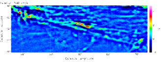
In Sect. 5.4.1 we discussed apparent position shifts of the filaments in Fig. 10 with changes in the observed radial velocity. Such shifts are frequent. In Fig. 25 we show another case at . This filament has at km s-1 almost no bending. It is not possible to argue for a convex shape and a blast wave origin.
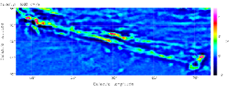
In Fig. 26 we give details of a prominent loop at . Significant shifts in position are easily visible in the USM channel maps. At more positive velocities the filaments tend to break into substructures.

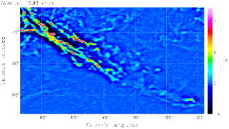
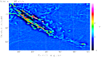
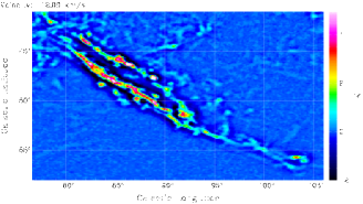
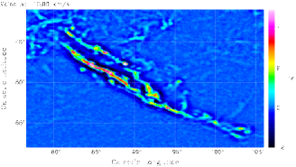
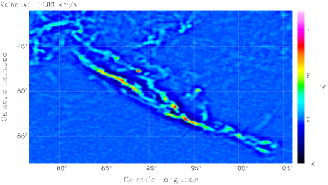
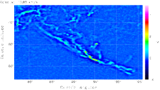
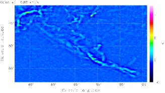
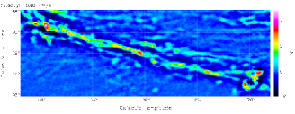
In Fig. 27 we present a filamentary structure that shows for velocity changes obvious gradients in the Hi distribution along the filaments.