Mean-variance risk-averse optimal control of systems governed by PDEs with random parameter fields using quadratic approximations††thanks: This work was partially supported by NSF grants 1508713 and 1507009, and DOE grants DE-FC02-13ER26128, DE-SC0010518, and DE-FC02-11ER26052.
Abstract
We present a method for optimal control of systems governed by partial differential equations (PDEs) with uncertain parameter fields. We consider an objective function that involves the mean and variance of the control objective, leading to a risk-averse optimal control problem. Conventional numerical methods for optimization under uncertainty are prohibitive when applied to this problem. To make the optimal control problem tractable, we invoke a quadratic Taylor series approximation of the control objective with respect to the uncertain parameter field. This enables deriving explicit expressions for the mean and variance of the control objective in terms of its gradients and Hessians with respect to the uncertain parameter. The risk-averse optimal control problem is then formulated as a PDE-constrained optimization problem with constraints given by the forward and adjoint PDEs defining these gradients and Hessians. The expressions for the mean and variance of the control objective under the quadratic approximation involve the trace of the (preconditioned) Hessian, and are thus prohibitive to evaluate. To overcome this difficulty, we employ trace estimators, which only require a modest number of Hessian-vector products. We illustrate our approach with two specific problems: the control of a semilinear elliptic PDE with an uncertain boundary source term, and the control of a linear elliptic PDE with an uncertain coefficient field. For the latter problem, we derive adjoint-based expressions for efficient computation of the gradient of the risk-averse objective with respect to the controls. Along with the quadratic approximation and trace estimation, this ensures that the cost of computing the risk-averse objective and its gradient with respect to the control—measured in the number of PDE solves—is independent of the (discretized) parameter and control dimensions, and depends only on the number of random vectors employed in the trace estimation, leading to an efficient quasi-Newton method for solving the optimal control problem. Finally, we present a comprehensive numerical study of an optimal control problem for fluid flow in a porous medium with uncertain permeability field.
keywords:
Optimization under uncertainty, PDE-constrained optimization, optimal control, risk-aversion, PDEs with random coefficients, Gaussian measure, Hessian, trace estimatorsAMS:
60H15, 60H35, 35Q93, 35R60, 65K101 Introduction
An important class of problems arising in engineering and science is the optimization or optimal control of natural or engineered systems governed by partial differential equations (PDEs). Often, the PDE models of these systems are characterized by parameters (or parameter functions) that are not known and are considered uncertain and modeled as random variables. These parameters can appear for example as coefficients, boundary data, initial conditions, or source terms. Consequently, optimization of such systems should be done in a way that the computed optimal controls or designs are robust with respect to the variability in the uncertain parameters.
Literature survey and challenges
There is a rich body of literature on theoretical and computational aspects of optimal control of systems governed by PDEs [45, 25, 5, 9, 27], and of optimization under uncertainty (OUU) [6, 40, 4, 41]. Recently there has been considerable interest in solution methods for optimization problems lying at the intersection of these two fields, namely, optimization problems governed by PDEs with uncertain parameters [10, 9, 11, 26, 28, 44, 29, 32, 31, 34, 30, 13, 33, 16]. To discuss the challenges of optimal control, and more generally optimization, of systems governed by PDEs with uncertain parameters, we consider a real-valued optimization objective that depends on a control variable and an uncertain parameter , both of which can be finite- or infinite-dimensional. Throughout this article we refer to as the control objective. The evaluation of this control objective requires the solution of a system of PDEs. Namely, with , where is a PDE solution operator. Here, we assumed that the system of PDEs admits a unique solution for every pair of controls and parameters. This dependence of on the solution of a PDE makes the evaluation (and the computation of derivatives) of computationally expensive. The presence of uncertain parameters greatly compounds the computational challenges of solving the PDE-constrained optimization problem.
In an OUU problem, it is natural to seek optimal controls that make small in an average sense. For example, a risk-neutral optimal control approach seeks controls that solve
| (1) |
where denotes expectation over the uncertain parameter . If we seek controls that, in addition to minimizing the expected value of with respect to , result in a small uncertainty in , we are led to risk-averse optimal control. In the present work, we use the variance of the control objective as a risk measure, and seek optimal controls that solve the problem
| (2) |
Here, denotes the variance with respect to , and is a risk-aversion parameter that aims to penalize large variances of the control objective. This mean-variance formulation is only one of several formulations for finding risk-averse optimal controls. Other examples of more complex risk measures include the value at risk (VaR) and the conditional value at risk (CVaR) [37, 41]. Compared to the mean-variance formulation, these approaches do not symmetrically penalize the deviation of the quantity of interest around the mean, which is desirable for instance in applications where the control objective models a loss. In [33], the authors consider primal and dual formulations of a risk-averse PDE-constrained OUU problem using CVaR. They employ and study smooth approximations of the primal formulation to enable the application of derivative-based optimization methods to the CVaR objective, and rely on quadrature-based discretizations in the discretized parameter space.
To illustrate the main computational challenges involved in OUU problems, let us consider the (simpler) risk-neutral problem. A common approach to cope with the expectation in the objective function uses sampling over the random parameter space, , where is a sample set, and are sample weights. In the context of PDE-constrained OUU, evaluation of requires solving the PDE problem for each sample point . The sample set is chosen either by Monte Carlo sampling, where each is a draw from the distribution law of (and for every ), or, for a suitably low-dimensional parameter space, based on quadrature rules (and are quadrature weights). The Monte Carlo-based approach, sometimes referred to as sample average approximation (SAA), is computationally prohibitive for OUU problems governed by PDEs. This is due to the slow convergence of Monte Carlo and the resulting large number of PDE solves for each evaluation of the expectation. Quadrature-based methods, obtained from tensorization of one-dimensional quadrature rules, use regularity of with respect to and can accelerate convergence, but they suffer from the the curse of dimensionality—the exponential growth of the number of quadrature points as the dimension increases. The use of sparse quadrature [42] can mitigate but not overcome the curse of dimensionality. Quadrature-based methods can be improved significantly by using adaptive sparse grids (see e.g., [32, 9, 31], in which adaptive sparse grids are employed to solve OUU problems); however these approaches are still computationally expensive for problems with parameter dimensions in the order of hundreds or thousands. Another class of methods for OUU problems are stochastic approximation (SA) methods [36, 24, 22, 39]. Similar to methods based on SAA, SA methods are computationally intractable for PDE-constrained OUU problems with high-dimensional parameters due to their slow convergence and the resulting need for a prohibitively large number of PDE solves.
Approach
We consider an uncertain parameter that is modeled with a random field, which can also be viewed as a function-valued random variable. In the uncertainty quantification literature, it is a common to use an a priori dimension reduction provided by a truncated Karhunen–Loève (KL) decomposition for such problems. However, KL modes that appear unimportant in simulating the random process may turn out to be important to the control objective. Moreover, a priori truncation of the KL expansion of a random field is most useful if the eigenvalues of the covariance operator (of the uncertain parameter) exhibit rapid decay. This is not always the case, for example, in presence of small correlation lengths; in such cases, an a priori truncation needs to retain a large number of KL modes. We do not follow such approaches to avoid bias introduced by the truncated KL expansion. Instead, we seek formulations that preserve the problem’s infinite-dimensional character and work in an infinite-dimensional setting as long as possible. Moreover, we aim to devise algorithms whose computational complexity, measured in the number of PDE solves, is independent of the discretized parameter dimension.
In the present work, we employ quadratic approximations of the parameter-to-objective map, , to render the computation of the control objective and its gradient (as necessitated by a gradient-based optimization method) tractable. Related approaches for OUU with finite-dimensional uncertain parameters and inexpensive-to-evaluate (compared to problems governed by PDEs) control objectives are used in [18, 17]. More generally, linear or quadratic expansions with respect to uncertain finite-dimensional parameters have also been used for robust (finite-dimensional) optimization and reliability methods in engineering applications; we refer, e.g., to [21, 35]. Using this approach, we can compute the moments of the first and second-order Taylor expansions of analytically. For optimal control problems with infinite-dimensional parameters, computation of the derivatives with respect to the uncertain parameters and the controls is prohibitive using the direct sensitivity approach (or finite differences). Instead, we employ adjoint methods to avoid dependence on the dimension of the discretized parameter field. Our formulation is particularized to two model problems, the control of a semilinear elliptic PDE with an uncertain boundary source term, and the control of a linear elliptic PDE with an uncertain coefficient field. The latter is motivated by industrial problems involving the optimal control of flows in porous media.
As we will see, using the quadratic approximation of results in an OUU objective function that involves traces of operators that depend on the Hessian of this mapping. Since direct computation of these traces is prohibitive for high-dimensional problems (explicit computation of the Hessian requires as many PDE solves as there are parameters), we use trace estimation either based on random vectors, or on eigenvectors of the (preconditioned) Hessian at a nominal control. This only requires the action of the Hessian on vectors and is thus well suited for control problems governed by systems of PDEs.
Contributions
The main contributions of this work are as follows: (1) For an uncertain parameter field that follows a Gaussian distribution law, we derive analytic expressions for the mean and variance of a quadratic approximation to the parameter-to-objective map in infinite dimensions. These results are the basis for developing an efficient OUU approach that extends the work in [17] to a method suitable for large-scale PDE-constrained OUU problems. (2) We propose a formulation of the risk-averse OUU problem as a PDE-constrained optimization problem, with the constraints given by the PDEs defining the adjoint-based expression for the gradient and the linear action of the Hessian of the parameter-to-objective map. Our method ensures that the cost of computing the risk-averse objective and its gradient with respect to the control—measured in the number of PDE solves—is independent of the (discretized) parameter and control dimensions, and depends only on the number of random vectors used in the trace estimation. (3) We fully elaborate our approach for the risk-averse control of an elliptic PDE with uncertain coefficient field, and in particular derive the adjoint-based gradient of the control objective with respect to the control. We numerically study various aspects of our risk-aversion measure and of the efficiency of the method. The results show the effectiveness of our approach in computing risk-averse optimal controls in a problem with a -dimensional discretized parameter space.
Limitations
We also remark on limitations of our method. (1) Since we rely on approximations based on Taylor expansions, our arguments require smoothness (and proper boundedness of the derivatives) of the parameter-to-objective map. For the mean-variance formulation used here, this smoothness mainly depends on the governing PDEs and how the parameter enters these PDEs. (2) Compared to sampling-based methods, our approach requires first and second derivatives of with respect to , and thus appropriate adjoint solvers for the efficient computation of these derivatives. However, efficient methods for solution of optimal control problems governed by PDEs will require adjoint-based derivatives with respect to the control; only minor modifications are needed to obtain derivatives with respect to the uncertain parameters. (3) Our derivation of the mean and variance of the quadratic approximation to the parameter-to-objective map assumes that the parameter space is a Hilbert space, say , and that is defined and has the required derivatives in . As such, our framework does not apply to cases where the parameter space is a general Banach space. Even when we consider a Hilbert space of uncertain parameters, may not be defined for every in and have derivatives that are bounded in , in which case the expressions for the mean and variance could be used only formally to obtain an objective function for a risk-averse OUU problem. This is the case for the linear elliptic PDE problem with uncertain coefficient field, where the parameter-to-objective map is defined and has the required smoothness only in a subspace that has full measure. In section 3.3, we discuss such issues further and give conditions that ensure that the expressions for the mean and variance are well defined. Extensions to more general cases is a subject of our future work.
2 Preliminaries
We let be an infinite-dimensional real separable Hilbert space endowed with an inner product and induced norm . We consider uncertain parameters that are modeled as spatially distributed random processes, which can be viewed as function-valued random variables. Let denote such an uncertain parameter. We assume the distribution law of , which we denote by , is supported on and consider as an -valued random variable. That is, is a function, , where is a sample space, is an appropriate sigma-algebra, and is a probability measure; here, denotes the Borel sigma-algebra on . In what follows, with a slight abuse of notation, we denote the realizations of the uncertain parameter using the same symbol .
As is common practice, instead of working on the abstract probability space , we work in the image space , where is the law of , and use for an integrable function . As mentioned in the introduction, we assume that has a Gaussian probability law, . Here, is a self-adjoint, positive trace class operator and thus defines a Gaussian measure on .
We denote by the set of admissible controls, which is a closed convex subset of , where is a bounded open set with piecewise smooth boundary. We consider the control objective, as a real-valued function defined on . We refer to the mapping as the parameter-to-objective map. For normed linear spaces and we denote by the space of bounded linear transformations from to , and by the space of bounded linear operators on . For a Hilbert space , we use to denote the subspace of consisting of self-adjoint linear operators.
2.1 Linear and quadratic expansions
Recall that for a function , where is a Banach space, existence of first and second Fréchet derivatives at implies that
| (3) |
with and . In the following, we consider the case where is a Hilbert space , and hence the derivatives admit Riesz representers in .
Next, we consider the control objective, and assume for an arbitrary control , existence of first and second Fréchet derivatives for the parameter-to-objective map at . Consider the linear and quadratic approximations of the parameter-to-objective map:
| (4) | ||||
| (5) |
Notice that for clarity, we denote first and second derivatives of with respect to by and , respectively. In this paper, we mainly use the quadratic approximation .
Using an approximation rather than the exact parameter-to-objective map enables computing the moments appearing in the objective function of the (approximate) risk-averse OUU problem analytically. This computation is facilitated by the fact that has a Gaussian distribution law. Note also that the accuracy of such linear and quadratic approximations, considered in an average sense, can be related to the variance of the uncertain parameter. In section 3, where we derive analytic expressions for the mean and variance of the local quadratic approximation to , we also describe how the variance of is related to the expected value of the truncation error in the quadratic approximation.
2.2 Probability measures on
Here we recall basics regarding Borel probability measures, and Gaussian measures on infinite-dimensional Hilbert spaces. Let be a Borel probability measure on with finite first and second moments. The mean of is an element of such that,
The covariance operator of is a positive self-adjoint trace-class operator that satisfies
It is straightforward to show that , where denotes the trace of the (positive self-adjoint) operator ; see, e.g., [14, p. 8]. Note also that
| (6) |
One can also show (see e.g.,[1, Lemma 1]) that for a bounded linear operator ,
| (7) |
Now consider the case where the measure is a Gaussian, , where is a positive, self-adjoint, trace-class operator. The mean is assumed to belong to the Cameron–Martin space . The Cameron–Martin space is a dense subspace of and is a Hilbert space endowed with the inner product [15]. While the space is dense in , it is in some sense very “thin”; more precisely, .
We follow the construction in [12], and define a Gaussian measure on , where is a bounded domain with piecewise smooth boundary, as follows: define the covariance operator as the inverse of the square of a Laplacian-like operator:
| (8) |
where , and the domain of is given by . Here, is the Sobolev space of functions with square integrable first and second weak derivatives, and is the unit outward normal for the boundary . This construction of the operator ensures that it is positive, self-adjoint, and of trace-class and thus the Gaussian measure on is well-defined. A Gaussian random field whose law is given by such a Gaussian measure has almost surely continuous realizations [43].
As we saw in (7), given a Borel probability measure on with bounded first and second moments, we can obtain a simple expression for the first moment of a quadratic form on . If is a Gaussian measure on , we can also compute the second moment of a quadratic form (see Remark 1.2.9. in [15]). In particular, if we let be a self-adjoint bounded linear operator on , then
| (9) |
3 Risk-averse OUU with quadratic approximation of the parameter-to-objective map
As discussed above, we consider a control objective , where has a Gaussian distribution law . In section 3.1, we analytically derive the moments of the quadratic approximation of . We discuss the approximation errors due to this approximation by studying the expected value of the remainder term in the Taylor expansion. In section 3.2, using the expressions for the moments of the quadratic approximation, we formulate the optimization problem for finding risk-averse optimal controls. Extensions of our OUU approach to problems where is defined only in a subspace of are discussed in section 3.3.
3.1 Quadratic approximation to a function of a Gaussian random variable
In this section, we compute mean and variance of defined in (5) in the infinite-dimensional Hilbert space setting. The following arguments are pointwise in the control and hence, for notational convenience, we suppress the dependence of on . We begin by establishing the following technical result:
Lemma 1.
Let be a Gaussian measure on , and be fixed, and let be a bounded linear operator on . Then,
Proof.
Without loss of generality, we assume . Let be an orthonormal basis of eigenvectors of with corresponding positive eigenvalues . By we denote the orthogonal projection onto the span of the first eigenvectors. Observe that , and that . Since , we can apply the Lebesgue Dominated Convergence Theorem to obtain
where in the last step we used that the random -vector defined by is an -variate Gaussian whose distribution law is . Note that we also use the result (see, e.g., [46]) that for a mean zero -variate normal random vector , for .
3.1.1 Mean and variance of the quadratic approximation
Next, we derive expressions for the mean and variance of in the infinite-dimensional Hilbert space setting.
Proposition 2.
Let be a function that is twice differentiable at , with gradient and Hessian . Let be as defined in (5). Then,
| (10) | ||||
| (11) |
Proof.
The first statement follows from,
To derive the expression for the variance, first note that the variance of equals the variance of . Thus,
| (12) |
The first term on the right hand side is given by
This, along with and (12) finishes the proof.
Note that the expressions for the mean and variance of the linear approximation defined in (4) consist of only the first terms in (10) and (11), respectively. We also point out an intuitive interpretation of the covariance-preconditioned Hessian, , in the expressions for the mean and variance in (10) and (11). As the Hessian only appears preconditioned by the covariance , the second-order contributions to the expectation and the variance are large only if the dominating eigenvector directions of and are “similar”. More precisely, the eigenvectors of that correspond to large eigenvalues (i.e., directions of large uncertainty) only have a significant influence on the mean and variance if these directions are also important for the Hessian of the prediction. Conversely, important directions for the prediction Hessian only result in significant contributions to the second-order approximation of mean and variance if the uncertainty in these directions is significant.
We point out that while the Gaussian assumption on the distribution law of is required for derivation of the expression for in Proposition 2, the expression for can be derived without this assumption. Namely, it holds if the law of is any Borel probability measure on with bounded first and second moments. These assumptions on the law of are also sufficient for deriving the expressions for the mean and variance of ,
Here, the expression for the mean is immediate and the one for variance follows from (6).
3.1.2 Expected value of the truncation error
Next, we discuss the error due to replacing by the quadratic approximation . Assuming sufficient smoothness and boundedness of the derivatives of , we study the expected value of the truncation error as the uncertainty in the parameter decreases, i.e., we consider , where approaches zero. To gain intuition, consider the case when the covariance operator is such that parameter draws have a high probability of being close to the mean , where the quadratic approximation is more accurate. In this case, we can expect the truncation error to be small.
To derive a quantitative estimate, we assume that is three times continuously differentiable such that the remainder term in the quadratic expansion (3) has the form:
| (13) |
Here, denotes the third derivative with respect to at , which is an element of the line segment between and . Note that this and the following considerations are pointwise in the control variable . We are interested in the expectation value of the remainder term, which we will relate to , the average variance of .
Assuming is a uniformly bounded trilinear map, i.e., for all , we obtain
| (14) |
Next, recall that . Moreover, using (9) with , we have
| (15) |
where we have also used . Therefore, using (14) and (15), we have
Now, if we consider a family of laws , , for , then, the expected value of the remainder (13) is , as . This should be contrasted with the expected value of the remainder term for the linear expansion which can be shown to be . Note that if is cubic, the third derivative is constant and the expectation over the remainder term vanishes since follows a Gaussian distribution that is symmetric with respect to its mean.
The above argument regarding the expected value of the remainder in a Taylor expansion can be generalized for higher order expansions; see appendix A.
3.2 The OUU objective function
We can now give the explicit form for the objective function for the risk-averse OUU problem (2), in which we use rather than , and thus (10) and (11):
| (16) |
Note that we have also added the control cost in (16). The numerical computation of operator traces appearing in the expressions for the mean and variance of the quadratic approximation is expensive and can be prohibitive for inverse problems governed by PDEs. Hence, we employ approximations obtained by randomized trace estimators [3, 38], which require only the application of the operator to (random) vectors and provide reasonably accurate trace estimates using a small number of trace estimator vectors (see also [2, Appendix A] for a result on an infinite-dimensional Gaussian trace estimator). Trace estimation for and amounts to
| (17) | ||||
where , are draws from the measure . This form of the trace estimators is justified by the identities
Replacing the operator traces in the OUU objective function (16) using trace estimators results in the OUU objective function
| (18a) | ||||
| where for , | ||||
| (18b) | ||||
As an alternative to the randomized estimator in (17), we can use
with , where is an orthonormal basis of , and is an appropriate truncation level. One possibility is to choose , as the dominant eigenvectors of , where is a nominal control variable. Since in many applications the operator has a rapidly decaying spectrum, can be chosen small. While such an estimator is tailored to the Hessian evaluated at , we have observed it to perform well for values of the control variable in a neighborhood of . We will demonstrate the utility of this approach in our computational results.
Note that the existence of minimizers for (as well as (16)) depends on the control space and on properties of and , and must be argued on a case-by-case basis.
3.3 Extensions
In some applications, the control objective might be defined only for in a Banach subspace with . Let be such a subspace, and recall that since the Cameron–Martin space is compactly embedded in all subspaces of that have full measure [43], is compactly embedded in . Moreover, when using quadratic approximations, we need derivatives at . It is thus reasonable to require existence of derivatives only in the Cameron–Martin space. In such cases, one might be tempted to consider the restriction of to the Cameron–Martin space and use
| (19) |
Here denotes the duality pairing between and its dual , and and are the gradient and Hessian of at , respectively. Note that we have suppressed the dependence of on .
The definition (19), however, is not meaningful from a measure-theoretic point of view as has measure zero. A possible remedy is to define a bounded and self-adjoint linear operator and to consider the composition . One possibility is to choose , in which case the smoothing is controlled by . The gradient and Hessian of are now given by
This way, one might consider the local quadratic approximation
This construction allows to consider control objectives that are defined only on to be extended to via the mapping . Then, the Hilbert space formulation of the risk-averse OUU with quadratic approximations, developed in earlier sections, can be applied.
Another case where the Hilbert space theory needs extension is when is defined on a Banach subspace of full measure, and thus its gradient and Hessian belong to and , respectively. For example, in the control problem governed by a linear elliptic PDE with uncertain coefficient discussed in section 5, the space plays such a role (it is known [43, 19] that due to our choice of the covariance operator , ). In this case, we show that the expressions for the mean and variance of the quadratic approximation continue—under appropriate assumptions—to be well-defined.
Now, the gradient , and thus can be interpreted as a duality product, i.e., the linear action of on . Here, we have used that for the covariance operator defined above, we have .
Next, considering the expressions (10) and (11) for mean and variance, it remains to specify conditions that ensure that the operator is trace-class on .
Proposition 3.
Let be the covariance operator as defined in section 2.2. Assume that restricted to is a bounded linear operator on . Then, the operator is a trace class operator on .
Proof.
It is straightforward to see that . It remains to show that is trace-class. Let be the complete orthonormal set of eigenvectors of , with corresponding (positive) eigenvalues . We note that for , . Therefore, for each , we can write
Therefore, .
4 Control of a semilinear elliptic PDE with uncertain Neumann boundary data
We first illustrate our approach for the optimal control of a semilinear elliptic PDE with uncertain Neumann boundary data and a right hand side control. In this problem, the nonlinearity in the governing PDE is the sole reason why the quadratic approximation of the objective is not exact. Below, we present and discuss the optimization formulation for this PDE-constrained OUU problem.
We assume a bounded domain with boundary split into disjoint parts and , and we consider the semilinear elliptic equation
| in | (20) | |||||
| on | ||||||
| on |
Here, , is the control and the uncertain parameter is , distributed according to the law with mean and covariance operator . Due to the monotonicity of the nonlinear term, the state equation (20) has a unique solution for every Neumann data and every , [20].
We consider a control objective of tracking type as follows:
| (21) |
where is a given desired state. It is straightforward to show that the solution of (20) satisfies the estimate , for a constant . Hence, since has moments of all orders, it follows that the state variable also has moments of all orders for every . This in particular implies the existence of the first and second moments of the control objective for every . Therefore, a mean-variance risk-averse OUU objective function is well-defined.
To derive the quadratic approximation of (21) with respect to at the mean , we compute, for fixed control , the gradient and Hessian of with respect to . The gradient of with respect to is , where satisfies (20) with (the corresponding state is denoted by ), and satisfies the adjoint equation
| in | (22) | |||||
| on | ||||||
| on |
The second derivative at evaluated in a direction is given by , where solves the incremental adjoint equation:
| in | (23) | |||||
| on | ||||||
| on |
and the incremental state equation:
| in | (24) | |||||
| on | ||||||
| on |
We now show that is bounded as mapping from . From (24) it follows that . To estimate the -norm of the right hand side in (23), we consider an arbitrary . Using Hölder’s inequality and the continuous embedding of in , we obtain
where the constants do not depend on or . This shows that the -norm of the right hand side in (24) is bounded by . Hence, with constants :
which proves the boundedness of . Thus, the OUU objective function (16), specialized to the present example, with the gradient and Hessian operators and defined above is well-defined and conforms to the theory outlined in sections 3.1–3.2.
5 Control of an elliptic PDE with uncertain coefficient
Motivated by problems involving the optimal control of flows in porous media, we consider the optimal control of a linear elliptic PDE with uncertain coefficient field. We discuss this application numerically in section 6, where we consider control of fluid injection into the subsurface at injection wells. In this section, we describe the control objective and the PDE-constrained objective function for the risk-averse OUU problem, and derive the adjoint-based expressions for the gradient of the OUU objective function. This is an example for a problem in which the parameter-to-objective map is defined only on a Banach subspace of that has full measure. We thus use the expressions for the mean and variance of the quadratic approximation, developed in a Hilbert space setting in section 3, formally, to define the objective function for the risk-averse optimal control problem.
We begin by describing the state (forward) equation. On an open bounded and sufficiently smooth domain , with boundary , we consider the following elliptic partial differential equation:
| (25) | ||||||
Here, the boundary is split into disjoint parts and on which we impose Dirichlet and Neumann boundary conditions, respectively. The Dirichlet data is , denotes the unit-length outward normal for the boundary , and for simplicity we have considered homogeneous Neumann conditions. We assume that the right hand side is specified as , where is a bounded linear transformation and is a distributed source per unit volume.
We consider the weak form of (25), i.e., we seek solutions that satisfy
| (26) |
We consider the case where the log-permeability, , is uncertain and is modeled as a spatially distributed random field; see also [19, 7]. The realizations of belong to the Hilbert space , and we assume is distributed according to a Gaussian with covariance operator and mean , where is the Cameron–Martin space associated with the Gaussian measure . With our choice of the covariance operator, with .
We consider the following tracking-type control objective :
| (27) |
where solves the weak form of the state equation (26), is a bounded linear operator, and is given. Notice that this control objective is defined for every , i.e., almost surely. It is also possible to prove boundedness of moments of , which, in particular, ensures that a mean-variance risk-averse OUU objective based on (27) is well-defined. Compared to the problem discussed in section 4, here the proof of boundedness of moments of is more involved (see [19, Example 2.15]) and requires the use of Fernique’s theorem [23].
For fixed parameter and control , the gradient of the parameter-to-objective map can be computed with a standard variational calculus approach (see, e.g., [8]). In particular, at , the gradient is given by
| (28) |
where is the solution to the state equation, and solves the adjoint equation, i.e., and satisfies
| (29) |
Similarly, the action of the Hessian, in a direction can be expressed as
| (30) |
where and are the state and adjoint variables computed with a given control at . The variables and , which we refer to as the incremental state and adjoint variables, are obtained by solving the following incremental state and adjoint equations:
| (31a) | ||||
| (31b) | ||||
Note that (28) and (30) for and require that the state and adjoint equations (25) and (29), as well as their incremental variants (31), are satisfied. Thus, in the formulation of the OUU objective function (18a), these equations must be enforced as constraints.
5.1 The OUU problem for (25)
Here we summarize the formulation of the OUU problem, which uses a quadratic approximation of defined in (27):
| (32a) | |||||
| where for | |||||
| (32b) | |||||
| (32c) | |||||
| and the variables , which can be considered the state variables of the OUU problem, solve | |||||
| (32d) | |||||
| (32e) | |||||
| (32f) | |||||
| (32g) | |||||
5.2 Evaluation and gradient computation of the OUU objective function
Solving the PDE-constrained optimization problem (32) efficiently requires gradient-based optimization methods. To compute the gradient of with respect to , we follow a Lagrangian approach, and employ adjoint variables (i.e., Lagrange multipliers) to enforce the PDE constraints (32d)–(32g). The details of the derivation of the gradient are relegated to appendix B. The expression for the gradient, in a direction , takes the form:
| (33) |
where is obtained by solving the following system of equations for the OUU adjoint variables
| (34a) | ||||
| (34b) | ||||
| (34c) | ||||
| (34d) | ||||
for all , with , and given by
Next, we count the number of PDE solves required for the evaluation of the objective function (32a) and of its gradient (33). Although in the present example, the application of requires PDE solves that are similar to those in the state and adjoint equations, we do not include them in our counting since (1) the matrix in does not change and thus a sparse factorization or multigrid solver can be set up upfront, and (2) we aim at problems where the state (and thus the adjoint) equation is more complex than in the present case and thus its solution dominates the application of .
Hence, the number of forward-like PDE solves (i.e., the state equations, the adjoint equation, and incremental equations) required for evaluating the objective function (32a) is . The gradient evaluation requires another PDE solves. Thus, PDE solves are necessary for evaluating the OUU objective function and its gradient. If a small provides an approximation of the trace that is suitable for computing an optimal control, each iteration of a gradient-based method requires a moderate, fixed number of PDE solves. We demonstrate this in our numerical experiments, where for a typical OUU problem with a discretized parameter dimension of about , PDE solves are required for approximating the OUU objective and its gradient. This modest computational cost should be contrasted with methods that approximate the OUU objective using sampling or quadrature in the parameter space. While these approaches can, asymptotically, solve the original OUU problem rather than the formulation based on the quadratic expansion of , their cost in terms of PDE solves can be much higher. Moreover, if a factorization-based direct solver can be used for the governing PDE problems, these factorizations can be reused multiple times in the quadratic approximation approach. This is the case since the PDE operators arising in each quadratic approximation correspond to the same parameter. Thus, reusing factorizations can save significant computation time. Since each sample in the Monte Carlo approach corresponds to a different parameter, matrix factorizations must be recomputed for each sample.
The computational cost of sampling-based methods is exacerbated for OUU problems governed by nonlinear forward PDEs; in such cases, while our approach requires only one nonlinear PDE solve and linear(ized) PDE solves (for OUU objective and gradient evaluation), the required number of nonlinear PDE solves for sampling approaches scales with the number of samples.
6 Computational experiments
Next, we numerically study our OUU approach applied to the control of an elliptic PDE with an uncertain coefficient as discussed in section 5.
6.1 Problem setup
We consider a rectangular domain for (25), impose Dirichlet boundary conditions on the left and right sides of the domain according to and for , and use homogeneous Neumann boundary conditions on the top and bottom boundaries. We use a finite element mesh with linear rectangular elements and degrees of freedom to discretize the state and adjoint variables, and the uncertain parameter field. The discretized uncertain parameters are the coefficients in the finite element expansion of the parameter field.
The probability law of the uncertain parameter field
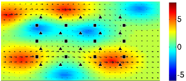
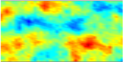
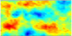
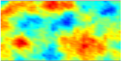
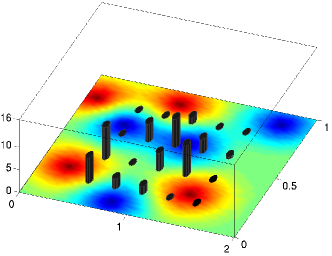
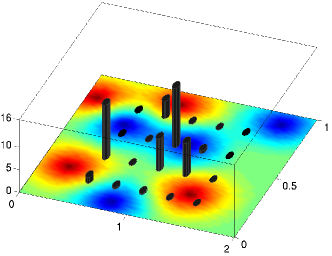
The probability law of the uncertain parameter, which is the log-permeability field , is given by a Gaussian measure . The mean and the locations of production and control wells are shown in Figure 1 (upper left image). The covariance operator of is as in (8), with and . These values are chosen such that samples from have a desired magnitude and correlation length. Typical realizations of the random process are also shown in Figure 1.
The control
For the right hand side in (25), we consider , and define as a weighted sum of finitely many mollified Dirac delta functions, which we denote by , :
| (35) |
The weights in (35) are the (finitely many) control variables, summarized in the control vector . The right hand side (35) is motivated by subsurface flow applications in petroleum engineering, where fluid injection at injection wells is used to control the flow rates at production wells. Here, represent the locations of injection wells, and are the injection rates at these wells. We impose control bounds, i.e., the set of admissible controls is
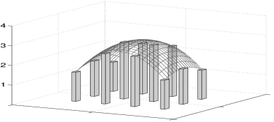
where and . In the present example, we use control wells; see Figure 1 (top left). The control objective (27) is the squared difference between the pressure at the production wells and a vector of target pressure values, which follows a parabolic profile as depicted in Figure 1 (top right).
Quadratic approximations in the small variance limit
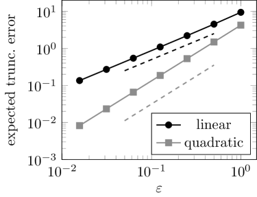
Here, we compare approximation error in the linear and quadratic approximations of the parameter-to-objective map, at a fixed control with for , in the sense discussed in section 3.1.2. In Figure 2, we consider the expected value of the truncation error of the first and second-order Taylor expansion to the mapping . This illustrates the rate of decay of the expected truncation error as indicated by the analysis in section 3.1.2. In particular, the truncation error in a linear expansion is and that of the quadratic approximation is . In this study, we consider scaling the distribution law of given according to with successively smaller values of .
6.2 Results
We solve the numerical optimization problem (32) via an
interior point method (to incorporate the box constraints for
) with BFGS Hessian approximation. For that purpose, we
employ MATLAB’s
fmincon routine, to which we provide functions for the
evaluation of the objective function (32) and for the
computation of its gradient with respect to the control, as derived in
the previous section.
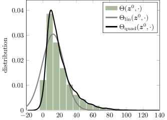
We use a uniform control vector (see Figure 3 left) as the initial guess of the optimization algorithm. It is instructive to consider the statistical distribution of the control objective (as defined in (27)) for this initialization, which is shown in the right image in Figure 3. We also depict the distributions of the linear and quadratic approximations and as defined in (4) and (5), respectively. For all figures, we have used kernel density estimation (KDE) to approximate the probability density functions (PDFs) from 10,000 samples. Note that compared to , the distribution of is a significantly better approximation for the distribution of .
 |
 |
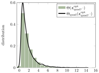
In Figure 4 we show the risk-averse optimal control for the risk-aversion parameter , the control cost weight , and where we use trace estimator vectors for approximating the traces in the OUU objective function. To cope with the nonconvexity of the OUU objective function, we use a continuation strategy with respect to , i.e., we solve a sequence of optimization problems with increasing , namely . The average number of quasi-Newton interior point iterations required to decrease the residual by was . The left figure shows the magnitude of the control vector at each injection well and the right figure depicts the statistical distribution of the control objective at the computed optimal control for both, and (note that the optimal control is based on the latter). To assess how successful the optimal control is in reducing the mean and the standard deviation, compare the right images in Figures 4 and 3. Notice that compared to the constant control , the optimal control results in a distribution of the objective that is both shifted to the left (reduction in the mean) and has less spread (reduction in variance).
 |
 |
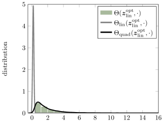
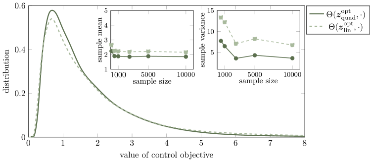
Next, we study if using the linear (rather than the quadratic) approximation to the parameter-to-objective map for the computation of risk-averse optimal control can lead to suboptimal results. Using instead of results in a simplified version of (32a), obtained by neglecting terms involving the Hessian . We solve the same risk-averse OUU problem as before but with rather than . The resulting optimal control is shown on the left of Figure 5, and the distributions of , and are shown on the right. Note the large discrepancy between the distributions; in particular the distribution based on is a poor approximation to the actual distribution. Our goal, however, is to find a control such that the distribution of the control objective has small mean and variance. In the present example, the optimal control computed with the linear approximation of the parameter-to-objective function does not perform much worse than the optimal control found with in terms of reducing the mean and variance of the distribution of —despite the poor approximation shown in Figure 5. This can be seen from Figure 6, where we compare the distribution of for the optimal controls and . We notice that the distribution of has slightly larger mean and variance, as can be observed by the thicker tail of the distribution.
Influence of risk-aversion parameter on the optimal control
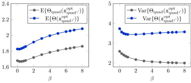
Next, we study the effect of the parameter in (32a) on the optimal control and the corresponding distribution of the control objective. In Figure 7, we show results for the mean and the variance for various risk-aversion parameters . While the optimal controls have been computed using , we also report the mean and variance of . With increasing the mean of increases and the variance of decreases, as expected. The optimal controls were computed using a fixed randomized trace estimator with .
Next, we consider the effect of increasing on the distribution of itself. While for small values, increasing results in smaller variances for , as desired, for larger values of , the variance increases with . This can be attributed to the fact that for computing the optimal control, we use the quadratic approximation , which only approximates the moments of the control objective .
Comparison between quadratic approximation and Monte Carlo
Next, we compare the computational cost for computing the optimal controls using the approach based on the quadratic approximation versus an SAA approach where Monte Carlo sampling is used to approximate (2). In Figure 8 (left), we plot the true OUU objective, approximated accurately using a large number of samples, against the cost per iteration measured in number of PDE solves required for objective and gradient computation, for three different risk-aversion parameters . For the quadratic approximation, we approximate the trace terms in the OUU objective function using randomized trace estimation (dash-dotted lines) and using eigenvectors of the covariance-preconditioned Hessian operator (solid lines), as described in Section 3.2. For the randomized trace estimation we use values in the range 1–100, and use the same trace estimator vectors for different values of ; for the eigenvector-based approach, we use . The eigenvectors are computed for a reference (namely the initial) control. The Monte Carlo sampling approach is shown with dashed line; for this approach, we use the same sequence of samples, for the different values of , with samples of size , , , , , and . Note that in the Monte Carlo approach, the cost per iteration for objective and gradient computation is twice the size of the Monte Carlo sample used.
For a more precise comparison, in Figure 8 (right) for each case we list the data values corresponding to the largest number of PDE solves. The figure in the left shows a few important results: (1) the eigenvector-based trace estimation outperforms the randomized trace estimation for all choices of ; in both cases, as the number of vectors used for the approximation of the trace increases, the function values level off, indicating convergence of the respective optimal controls; (2) the optimal controls computed using Monte Carlo sampling of the objective asymptotically converge to the exact optimal controls of the true OUU objective; hence, these controls will asymptotically outperform optimal controls based on the quadratic approximation; and (3) for low risk-aversion (i.e., small ) or for limited compute time (i.e., when only a small number of PDE-solves is afforded), the quadratic approximation approach is superior to the Monte Carlo SAA approach.
7 Conclusions
We propose a scalable method for risk-averse optimal control of systems governed by PDEs with uncertain parameter fields. Our approach uses a quadratic approximation of the parameter-to-objective map, which enables computing the moments appearing in the OUU objective function analytically. Moreover, we employ randomized trace estimators for the operator traces in the OUU objective function. The resulting optimization problem is constrained by the PDEs defining the gradient and the linear action of the Hessian . The resulting method for risk averse OUU is applicable to problems with high-dimensional discretized parameter spaces. This is demonstrated in numerical tests, where we present results for a problem with a -dimensional (discretized) parameter space. Hence, our approach provides a practical alternative to computationally expensive sampling-based OUU methods. The advantages of our method compared to sampling/quadrature methods are even more pronounced in the context of risk-averse optimal control of systems governed by nonlinear PDEs. Whereas our approach requires only one nonlinear PDE solve and about linear(ized) PDE solves (to evaluate the OUU objective function), the required number of nonlinear PDE solves for sampling approaches scales with the number of samples.
Appendix A Expectation of the truncation error in a Taylor expansion
We begin by stating a well-known result [43, Theorem 6.6] regarding Gaussian measures on a Hilbert space.
Theorem 4.
Let be a Gaussian measure on a Hilbert space . For any integer , there is a constant such that,
| (36) |
Note that the above theorem, for the case of , follows from (15). Next, we define the notation for the action of a -linear map .
Lemma 5.
Let , and suppose is a symmetric -linear map, with , such that for all . Then, we have, for a positive constant .
Proof. For , the proof is straightforward. For , if is even, i.e., for , then where the last inequality follows from Theorem 4. Note that here with from (36). In the case for , we have,
Proposition 6.
Let be, almost surely, a times continuously differentiable function, and assume , with . Suppose has uniformly bounded derivatives. Then, the expected value of the truncation error of the th order Taylor expansion is .
Proof. Since is times continuously differentiable,
The remainder term is given by , where is in the interior of the line segment between and . Here we use the notation for the th derivative. Now by assumption of the proposition, is uniformly bounded on . Therefore, by Lemma 5 we get is .
Appendix B Derivation of the gradient of the OUU objective function
Here, we summarize the derivation of the gradient of the OUU objective function presented in (32a). To derive the expression for the gradient, we employ a formal Lagrangian approach [45, 8], which uses a Lagrangian function composed of the objective function (32a) with the PDE constraints (32d)–(32g) enforced through Lagrange multiplier functions. This Lagrangian function for the OUU problem is given by:
The variables are the OUU state variables and are the OUU adjoint variables, with . Requiring that variations of with respect to the OUU adjoint variables vanish, we recover the OUU state equations (32d)-(32g). The variations of with respect to the OUU state variables are
with . Letting these variations vanish, results in the OUU adjoint equations (34a)-(34d). Finally, the gradient for (32a) is given by,
| (37) |
References
- [1] A. Alexanderian, P. J. Gloor, and O. Ghattas, On Bayesian A-and D-optimal experimental designs in infinite dimensions, Bayesian Analysis, 11 (2016), pp. 671–695. arXiv preprint arXiv:1408.6323.
- [2] A. Alexanderian, N. Petra, G. Stadler, and O. Ghattas, A fast and scalable method for A-optimal design of experiments for infinite-dimensional Bayesian nonlinear inverse problems, SIAM Journal on Scientific Computing, 38 (2016), pp. A243–A272.
- [3] H. Avron and S. Toledo, Randomized algorithms for estimating the trace of an implicit symmetric positive semi-definite matrix, Journal of the ACM (JACM), 58 (2011), p. 17.
- [4] H.-G. Beyer and B. Sendhoff, Robust optimization—a comprehensive survey, Computer Methods in Applied Mechanics and Engineering, 196 (2007), pp. 3190–3218.
- [5] L. T. Biegler, O. Ghattas, M. Heinkenschloss, D. Keyes, and B. van Bloemen Waanders, eds., Real-Time PDE-Constrained Optimization, SIAM, 2007.
- [6] J. R. Birge and F. Louveaux, Introduction to Stochastic Programming, Springer Verlag, Berlin, Heidelberg, New York, 1997.
- [7] F. Bonizzoni and F. Nobile, Perturbation analysis for the Darcy problem with log-normal permeability, SIAM/ASA Journal on Uncertainty Quantification, 2 (2014), pp. 223–244.
- [8] A. Borzì and V. Schulz, Computational Optimization of Systems Governed by Partial Differential Equations, SIAM, 2012.
- [9] A. Borzì, V. Schulz, C. Schillings, and G. Von Winckel, On the treatment of distributed uncertainties in PDE-constrained optimization, GAMM-Mitteilungen, 33 (2010), pp. 230–246.
- [10] A. Borzì and G. von Winckel, Multigrid methods and sparse-grid collocation techniques for parabolic optimal control problems with random coefficients, SIAM Journal on Scientific Computing, 31 (2009), pp. 2172–2192.
- [11] A. Borzì and G. von Winckel, A POD framework to determine robust controls in PDE optimization, Computing and visualization in science, 14 (2011), pp. 91–103.
- [12] T. Bui-Thanh, O. Ghattas, J. Martin, and G. Stadler, A computational framework for infinite-dimensional Bayesian inverse problems Part I: The linearized case, with application to global seismic inversion, SIAM Journal on Scientific Computing, 35 (2013), pp. A2494–A2523.
- [13] P. Chen and A. Quarteroni, Weighted reduced basis method for stochastic optimal control problems with elliptic PDE constraint, SIAM/ASA Journal on Uncertainty Quantification, 2 (2014), pp. 364–396.
- [14] G. Da Prato, An Introduction to Infinite-dimensional Analysis, Universitext, Springer, 2006.
- [15] G. Da Prato and J. Zabczyk, Second-order partial differential equations in Hilbert spaces, Cambridge University Press, 2002.
- [16] M. Dambrine, C. Dapogny, and H. Harbrecht, Shape optimization for quadratic functionals and states with random right-hand sides, SIAM Journal on Control and Optimization, 53 (2015), pp. 3081–3103.
- [17] J. Darlington, C. Pantelides, B. Rustem, and B. Tanyi, Decreasing the sensitivity of open-loop optimal solutions in decision making under uncertainty, European Journal of Operational Research, 121 (2000), pp. 343–362.
- [18] J. Darlington, C. C. Pantelides, B. Rustem, and B. A. Tanyi, An algorithm for constrained nonlinear optimization under uncertainty, Automatica, 35 (1999), pp. 217–228.
- [19] M. Dashti and A. M. Stuart, The Bayesian approach to inverse problems, in Handbook of Uncertainty Quantification, R. Ghanem, D. Higdon, and H. Owhadi, eds., Spinger, 2017.
- [20] J. C. De Los Reyes, Numerical PDE-constrained optimization, Springer, 2015.
- [21] M. Diehl, H. G. Bock, and E. Kostina, An approximation technique for robust nonlinear optimization, Mathematical Programming, 107 (2006), pp. 213–230.
- [22] Y. Ermoliev, Stochastic quasigradient methods and their application to system optimization, Stochastics, 9 (1983), pp. 1–36.
- [23] X. Fernique, Intégrabilité des vecteurs gaussiens, C. R. Acad. Sci. Paris Sér. A-B, 270 (1970), pp. A1698–A1699.
- [24] A. Gaivoronskii, Nonstationary stochastic programming problems, Cybernetics and Systems Analysis, 14 (1978), pp. 575–579.
- [25] M. D. Gunzburger, Perspectives in Flow Control and Optimization, SIAM, Philadelphia, 2003.
- [26] M. D. Gunzburger and J. Ming, Optimal control of stochastic flow over a backward-facing step using reduced-order modeling, SIAM Journal on Scientific Computing, 33 (2011), pp. 2641–2663.
- [27] M. Hinze, R. Pinnau, M. Ulbrich, and S. Ulbrich, Optimization with PDE Constraints, Springer, 2009.
- [28] L. S. Hou, J. Lee, and H. Manouzi, Finite element approximations of stochastic optimal control problems constrained by stochastic elliptic PDEs, Journal of Mathematical Analysis and Applications, 384 (2011), pp. 87–103.
- [29] D. Kouri, An Approach for the Adaptive Solution of Optimization Problems Governed by Partial Differential Equations with Uncertain Coefficients, PhD thesis, Rice University, 2012.
- [30] D. P. Kouri, A multilevel stochastic collocation algorithm for optimization of PDEs with uncertain coefficients, SIAM/ASA Journal on Uncertainty Quantification, 2 (2014), pp. 55–81.
- [31] D. P. Kouri, M. Heinkenschloss, D. Ridzal, and B. van Bloemen Waanders, Inexact objective function evaluations in a trust-region algorithm for PDE-constrained optimization under uncertainty, SIAM Journal on Scientific Computing, 36 (2014), pp. A3011–A3029.
- [32] D. P. Kouri, M. Heinkenschloss, D. Ridzal, and B. G. van Bloemen Waanders, A trust-region algorithm with adaptive stochastic collocation for PDE optimization under uncertainty, SIAM Journal on Scientific Computing, 35 (2013), pp. A1847–A1879.
- [33] D. P. Kouri and T. M. Surowiec, Risk-averse PDE-constrained optimization using the conditional value-at-risk, SIAM Journal on Optimization, 26 (2016), pp. 365–396.
- [34] A. Kunoth and C. Schwab, Analytic regularity and GPC approximation for control problems constrained by linear parametric elliptic and parabolic PDEs, SIAM Journal on Control and Optimization, 51 (2013), pp. 2442–2471.
- [35] R. Rackwitz, Reliability analysis–a review and some perspectives, Structural safety, 23 (2001), pp. 365–395.
- [36] H. Robbins and S. Monro, A stochastic approximation method, The annals of mathematical statistics, 22 (1951), pp. 400–407.
- [37] R. T. Rockafellar and S. Uryasev, Optimization of conditional value-at-risk, Journal of risk, 2 (2000), pp. 21–42.
- [38] F. Roosta-Khorasani and U. Ascher, Improved bounds on sample size for implicit matrix trace estimators, Foundations of Computational Mathematics, (2014), pp. 1–26.
- [39] A. Ruszczyński and W. Syski, A method of aggregate stochastic subgradients with on-line stepsize rules for convex stochastic programming problems, in Stochastic Programming 84 Part II, Springer, 1986, pp. 113–131.
- [40] N. V. Sahinidis, Optimization under uncertainty: state-of-the-art and opportunities, Computers & Chemical Engineering, 28 (2004), pp. 971–983.
- [41] A. Shapiro, D. Dentcheva, and A. Ruszczynski, Lectures on Stochastic Programming: Modeling and Theory, Society for Industrial and Applied Mathematics, 2009.
- [42] S. Smolyak, Quadrature and interpolation formulas for tensor products of certian classes of functions, Soviet Math. Dokl., 4 (1963), pp. 240–243.
- [43] A. M. Stuart, Inverse problems: A Bayesian perspective, Acta Numerica, 19 (2010), pp. 451–559.
- [44] H. Tiesler, R. M. Kirby, D. Xiu, and T. Preusser, Stochastic collocation for optimal control problems with stochastic pde constraints, SIAM Journal on Control and Optimization, 50 (2012), pp. 2659–2682.
- [45] F. Tröltzsch, Optimal Control of Partial Differential Equations: Theory, Methods and Applications, vol. 112 of Graduate Studies in Mathematics, American Mathematical Society, 2010.
- [46] C. Withers, The moments of the multivariate normal, Bulletin of the Australian Mathematical Society, 32 (1985), pp. 103–107.