New Stability and Exact Observability Conditions for Semilinear Wave Equations

Abstract

The problem of estimating the initial state of 1-D wave equations with globally Lipschitz nonlinearities from boundary measurements on a finite interval was solved recently by using the sequence of forward and backward observers, and deriving the upper bound for exact observability time in terms of Linear Matrix Inequalities (LMIs) [5]. In the present paper, we generalize this result to n-D wave equations on a hypercube. This extension includes new LMI-based exponential stability conditions for n-D wave equations, as well as an upper bound on the minimum exact observability time in terms of LMIs. For 1-D wave equations with locally Lipschitz nonlinearities, we find an estimate on the region of initial conditions that are guaranteed to be uniquely recovered from the measurements. The efficiency of the results is illustrated by numerical examples.

1 Introduction

Lyapunov-based solutions of various control problems for finite-dimensional systems can be formulated in the form of Linear Matrix Inequalities (LMIs) [3]. The LMI approach to distributed parameter systems is capable of utilizing nonlinearities and of providing the desired system performance (see e.g. [4, 7, 12]). For 1-D wave equations, several control problems were solved by using the direct Lyapunov method in terms of LMIs [8, 5]. However, there have not been yet LMI-based results for n-D wave equations, though the exponential stability of the n-D wave equations in bounded spatial domains has been studied in the literature via the direct Lyapunov method (see e.g. [18, 9, 1, 6]).

The problem of estimating the initial state of 1-D wave equations with globally Lipschitz nonlinearities from boundary measurements on a finite interval was solved recently by using the sequence of forward and backward observers, and deriving the upper bound for exact observability time in terms of LMIs [5]. In the present paper, we generalize this result to n-D wave equations on a hypercube. This extension includes new LMI-based exponential stability conditions for n-D wave equations. Their derivation is based on n-D extensions of the Wirtinger (Poincare) inequality [10] and of the Sobolev inequality with tight constants, which is crucial for the efficiency of the results. As in 1-D case, the continuous dependence of the reconstructed initial state on the measurements follows from the integral input-to-state stability of the corresponding error system, which is guaranteed by the LMIs for the exponential stability. Some preliminary results on global exact observability of multidimensional wave PDEs will be presented in [MashaCDC15].

Another objective of the present paper is to study regional exact observability for systems with locally Lipschitz in the state nonlinearities. Here we restrict our consideration to 1-D case, and find an estimate on the region of initial conditions that are guaranteed to be uniquely recovered from the measurements. Note that our result on the regional observability cannot be extended to multi-dimensional case (see Remark 4 below for explanation and for discussion on possible n-D extensions for different classes of nonlinearities). The efficiency of the results is illustrated by numerical examples.

The presented simple finite-dimensional LMI conditions complete the theoretical qualitative results of e.g. [15] (where exact observability of linear systems in a Hilbert space was studied via a sequence of forward and backward observers) and [2] (where local exact observability of abstract semilinear systems was considered).

Notation: $\mathbb{R}^{n}$ denotes the $n$-dimensional Euclidean space with the norm $|\cdot|$, $\mathbb{R}^{n\times m}$ is the space of $n\times m$ real matrices. The notation $P\!>\!0$ with $P\in\mathbb{R}^{n\times n}$ means that $P$ is symmetric and positive definite. For the symmetric matrix $M$, $\lambda_{min}(M)$ and $\lambda_{max}(M)$ denote the minimum and the maximum eigenvalues of $M$ respectively. The symmetric elements of the symmetric matrix will be denoted by ${*}$. Continuous functions (continuously differentiable) in all arguments, are referred to as of class $C$ (of class $C^{1}$). $L^{2}(\Omega)$ is the Hilbert space of square integrable $f:\Omega\to\mathbb{R}$, where $\Omega\subset\mathbb{R}^{n}$, with the norm $\|f\|_{L^{2}}=\sqrt{\int_{\Omega}|f(x)|^{2}dx}$. For the scalar smooth function $z=z(t,x_{1},\dots,x_{n})$ denote by $z_{t},z_{x_{k}},z_{tt},z_{x_{k}x_{j}}$ ($k,j=1,\dots n$) the corresponding partial derivatives. For $z:\Omega\to\mathbb{R}$ define $\nabla z=z_{x}^{T}=[z_{x_{1}}\ \dots z_{x_{n}}]^{T}$, $\Delta z=\sum_{p=1}^{n}z_{x_{p}x_{p}}$. ${\mathcal{H}}^{1}(\Omega)$ is the Sobolev space of absolutely continuous functions $z:\Omega\to\mathbb{R}$ with the square integrable $\nabla z$. ${\mathcal{H}}^{2}(\Omega)$ is the Sobolev space of scalar functions $z:\Omega\to\mathbb{R}$ with absolutely continuous $\nabla z$ and with $\Delta z\in L^{2}(\Omega)$.

2 Observers and exponential stability of n-D wave equations

2.1 System under study and Luenberger type observer

Throughout the paper we denote by $\Omega$ the n-D unit hypercube $[0,1]^{n}$ with the boundary $\Gamma$. We use the partition of the boundary:

$$\begin{array}[]{l}\Gamma_{D}\!=\!\{x\!=\!(x_{1},...,x_{n})^{T}\in\Gamma:\ \exists p\in{1,...,n}\ s.t.\ x_{p}=0\}\\ \Gamma_{N,p}=\{x\in\Gamma:\quad x_{p}=1\},\quad\Gamma_{N}=\bigcup_{p=1,\dots,n}\Gamma_{N,p}.\end{array}$$

Here subscripts D and N stand for Dirichlet and for Neumann boundary conditions respectively.

We consider the following boundary value problem for the scalar n-D wave equation:

$$\begin{array}[]{lll}z_{tt}(x,t)&=\Delta z(x,t)\!+\!f(z,x,t)\;in\;\Omega\times(t_{0},\infty),\\ z(x,t)&=0\qquad on\qquad\Gamma_{D}\times(t_{0},+\infty),\\ \frac{\partial}{\partial\nu}z(x,t)&=0\qquad on\qquad\Gamma_{N}\times(t_{0},\infty),\end{array}$$ (2.1)

where $f$ is a $C^{1}$ function, $\nu$ denotes the outer unit normal vector to the point $x\in\Gamma$ and $\frac{\partial}{\partial\nu}z$ is the normal derivative. Let $g_{1}>0$ be the known bound on the derivative of $f(z,x,t)$ with respect to $z$:

$$|f_{z}(z,x,t)|\leq g_{1}\quad\forall(z,x,t)\in\mbox{\Blackboard R}^{n+2}.$$ (2.2)

Since $\Omega$ is a unit hypercube, the boundary conditions on $\Gamma_{N}$ can be rewritten as

$$z_{x_{p}}(x,t)\Big{\rvert}_{x_{p}=1}=0\quad\forall x_{i}\in[0,1],\ i\neq p,\ p=1,\dots,n.$$

Consider the following initial conditions:

$$z(x,t_{0})=z_{0}(x),\ z_{t}(x,t_{0})=z_{1}(x),\quad x\in\Omega.$$ (2.3)

The boundary measurements are given by

$$y(x,t)=z_{t}(x,t)\qquad on\qquad\Gamma_{N}\times(t_{0},\infty).$$ (2.4)

Similar to [5], the boundary-value problem (2.1) can be represented as an abstract differential equation by defining the state $\zeta(t)=[\zeta_{0}(t)\ \zeta_{1}(t)]^{T}=[z(t)\ z_{t}(t)]^{T}$ and the operators

$$\begin{array}[]{lll}{\mathcal{A}}=\left[\begin{array}[]{cc}0&I\\ \Delta z&0\end{array}\right],\quad F(\zeta,t)=\left[\begin{array}[]{cc}0\\ F_{1}(\zeta_{0},t)\end{array}\right],\end{array}$$

where $F_{1}:{\mathcal{H}}^{1}(\Omega)\times R\to L^{2}(\Omega)$ is defined as $F_{1}(\zeta_{0},t)=f(\zeta_{0}(x),x,t)$ so that it is continuous in $t$ for each $\zeta_{0}\in{\mathcal{H}}^{1}(\Omega)$. The differential equation is

$$\dot{\zeta}(t)={\mathcal{A}}\zeta(t)+F(\zeta(t),t),\quad t\geq t_{0}$$ (2.5)

in the Hilbert space ${\mathcal{H}}={\mathcal{H}}_{\Gamma_{D}}^{1}(\Omega)\times L^{2}(\Omega)$, where

$${\mathcal{H}}^{1}_{\Gamma_{D}}(\Omega)=\left\{\zeta_{0}\in{\mathcal{H}}^{1}(\Omega)\ \bigg{|}\ {\zeta_{0}}_{|\Gamma_{D}}=0\right\}$$

and $\|\zeta\|^{2}_{\mathcal{H}}=\|\nabla\zeta_{0}\|^{2}_{L^{2}}+\|\zeta_{1}\|^{2}_{L^{2}}$. The operator ${\mathcal{A}}$ has the dense domain

$$\begin{array}[]{lll}{\mathcal{D}}({\mathcal{A}})=\!\!\Big{\{}&\!\!(\zeta_{0},\zeta_{1})^{T}\in{\mathcal{H}}_{\Gamma_{D}}^{1}(\Omega)\times{\mathcal{H}}_{\Gamma_{D}}^{1}(\Omega)\bigg{|}\ \Delta\zeta_{0}\in L^{2}(\Omega)\\ &{\rm and}\ \frac{\partial}{\partial\nu}{\zeta_{0}}_{|\Gamma_{N}}\!=-b{\zeta_{1}}_{|\Gamma_{N}}\!\Big{\}},\end{array}$$

where $b=0$. Here the boundary condition holds in a weak sense (as defined in Sect. 3.9 of [16]), i.e. the following relation holds:

$$\begin{array}[]{r}\langle\Delta\zeta_{0},\phi\rangle_{L^{2}(\Omega)}+\langle\nabla\zeta_{0},\nabla\phi\rangle_{[L^{2}(\Omega)]^{n}}=-b\langle\zeta_{0},\phi\rangle_{L^{2}(\Gamma_{N})}\\ \forall\phi\in{\mathcal{H}}_{\Gamma_{D}}^{1}(\Omega).\end{array}$$

The operator ${\mathcal{A}}$ is m-dissipative (see Proposition 3.9.2 of [16]) and hence it generates a strongly continuous semigroup. Due to (2.2), the following Lipschitz condition holds:

$$\begin{array}[]{lll}\|F_{1}(\zeta_{0},t)-F_{1}(\bar{\zeta}_{0},t)\|_{L^{2}}\leq g_{1}\|\zeta_{0}-\bar{\zeta}_{0}\|_{L^{2}}\end{array}$$ (2.6)

where $\zeta_{0},\bar{\zeta}_{0}\in{\mathcal{H}}^{1}_{\Gamma_{D}}(\Omega),t\in\mbox{\Blackboard R}.$ Then by Theorem 6.1.2 of [14], a unique continuous mild solution $\zeta(\cdot)$ of (2.5) in ${\mathcal{H}}$ initialized by

$$\begin{array}[]{ll}\zeta_{0}(t_{0})=z_{0}\in{\mathcal{H}}^{1}_{\Gamma_{D}}(\Omega),\ \zeta_{1}(t_{0})=z_{1}\in L^{2}(\Omega)\end{array}$$

exists in $C([t_{0},\infty),{\mathcal{H}})$. If $\zeta(t_{0})\in{\mathcal{D}}({\mathcal{A}})$, then this mild solution is in $C^{1}([t_{0},\infty),{\mathcal{H}})$ and it is a classical solution of (2.1) with $\zeta(t)\in{\mathcal{D}}({\mathcal{A}})$ (see Theorem 6.1.5 of [14]).

We suggest a Luenberger type observer of the form:

$$\widehat{z}_{tt}(x,t)=\Delta\widehat{z}(x,t)+f\Big{(}\widehat{z},x,t\Big{)},\qquad t\geq t_{0},\;x\in\Omega$$ (2.7)

under the initial conditions $[{\widehat{z}}(\cdot,t_{0}),{\widehat{z}}_{t}(\cdot,t_{0})]^{T}\in{\mathcal{H}}$ and the boundary conditions

$$\begin{array}[]{llll}\widehat{z}(x,t)&=0&on\ \Gamma_{D}\times(t_{0},\infty)\\ \frac{\partial}{\partial\nu}\widehat{z}(x,t)&=k\Big{[}y(x,t)-\widehat{z}_{t}(x,t)\Big{]}\!&on\ \Gamma_{N}\times(t_{0},\infty)\end{array}$$ (2.8)

where $k$ is the injection gain.

The well-posedness of (2.7), (2.8) will be established by showing the well-posedness of the estimation error $e=z-\widehat{z}$. Taking into account (2.1), (2.3) we obtain the following PDE for the estimation error $e=z-\widehat{z}$:

$$e_{tt}(x,t)=\Delta e(x,t)+ge(x,t)\quad t\geq t_{0},\quad x\in\Omega$$ (2.9)

under the boundary conditions

$$\begin{array}[]{lll}e(x,t)&=0&on\ \Gamma_{D}\times(t_{0},\infty)\\ \frac{\partial}{\partial\nu}e(x,t)&=-ke_{t}(x,t)&on\ \Gamma_{N}\times(t_{0},\infty).\end{array}$$ (2.10)

Here $ge=f(z,x,t)-f(z-e,x,t)$ and

$$\begin{array}[]{lll}g=g(z,e,x,t)=\int_{0}^{1}f_{z}(z+(\theta-1)e,x,t)d\theta.\end{array}$$

The initial conditions for the error are given by

$$\begin{array}[]{lll}e(x,t_{0})&=z_{1}(x)-z(\cdot,t_{0}),\\ e_{t}(x,t_{0})&=z_{2}(x)-z_{t}(\cdot,t_{0})\end{array}$$

The boundary conditions on $\Gamma_{N}$ can be presented as

$$\begin{array}[]{lll}e_{x_{p}}(x,t)\Big{\rvert}_{x_{p}=1}=-ke_{t}(x,t)\quad\forall x_{i}\in[0,1],\\ \ i\neq p,\ p=1,\dots,n.\end{array}$$

Let $z$ be a mild solution of (2.1). Then $z:[t_{0},\infty)\to{\mathcal{H}}^{1}$ is continuous and, thus, the function $F_{2}:{\mathcal{H}}^{1}\times[t_{0},\infty)\to L_{2}(0,1)$ defined as

$$F_{2}(\zeta_{0},t)=f(z,x,t)-f(z-\zeta_{0},x,t)$$

satisfies the Lipschitz condition (2.6), where $F_{1}$ is replaced by $F_{2}$. By the above arguments, where in the definition of ${\mathcal{D}}({\mathcal{A}})$ we have $b=k$, the error system (2.9), (2.10) has a unique mild solution $\{e,e_{t}\}\in C([t_{0},\infty),{\mathcal{H}})$ initialized by $[e(\cdot,t_{0}),e_{t}(\cdot,t_{0})]^{T}\in{\mathcal{H}}.$ Therefore, there exists a unique mild solution $\{\hat{z},\hat{z}_{t}\}\in C([t_{0},\infty),{\mathcal{H}})$ to the observer system (2.7), (2.8) with the initial conditions $[\hat{z}(\cdot,t_{0}),\hat{z}_{t}(\cdot,t_{0})]^{T}\in{\mathcal{H}}$. If $[e(\cdot,t_{0}),e_{t}(\cdot,t_{0})]^{T}\in{\mathcal{D}}({\mathcal{A}}),$ then $\{e,e_{t}\}\in C^{1}([t_{0},\infty),{\mathcal{H}})$ is a classical solution of 2.9), (2.10) with $[e(\cdot,t),e_{t}(\cdot,t)]\in{\mathcal{D}}({\mathcal{A}})$ for $t\geq t_{0}$. Hence, if $[\hat{z}(\cdot,t_{0}),\hat{z}_{t}(\cdot,t_{0})]^{T}\in{\mathcal{D}}({\mathcal{A}})$ and $[z_{0},z_{1}]^{T}\in{\mathcal{D}}({\mathcal{A}})$, there exists a unique classical solution $\{\hat{z},\hat{z}_{t}\}\in C^{1}([t_{0},\infty),{\mathcal{H}})$ to the observer system (2.7), (2.8) with $[\hat{z}(\cdot,t),\hat{z}_{t}(\cdot,t)]^{T}\in{\mathcal{D}}({\mathcal{A}})$ for $t\geq t_{0}$.

2.2 Lyapunov function and useful inequalities

We will derive further sufficient conditions for the exponential stability of the error wave equation (2.9) under the boundary conditions (2.10). Let

$$\begin{array}[]{ll}E(t)=\frac{1}{2}\int_{\Omega}\left[|\nabla e|^{2}+e_{t}^{2}\right]dx,\end{array}$$ (2.11)

be the energy of the system. Consider the following Lyapunov function for (2.9), (2.10):

$$\begin{array}[]{ll}V(t)=E(t)+\chi\int_{\Omega}\left[2(x^{T}\cdot\nabla e)+(n-1)e\right]e_{t}dx\\ \quad+\chi\frac{k(n-1)}{2}\int_{\Gamma_{N}}e^{2}d\Gamma\end{array}$$

with some constant $\chi>0$. Note that the above Lyapunov function without the last term was considered in [1, 6, 18]. The time derivative of this new term of $V$ cancels the same term with the opposite sign in the time derivative of $\chi\int_{\Omega}[(n-1)e]e_{t}dx$ (cf. (2.23) below) leading to LMI conditions for the exponential convergence of the error wave equation.

We will employ the following n-D extensions of the classical inequalities:

Lemma 1.

Consider $e\in{\mathcal{H}}^{1}(\Omega)$ such that $e\Big{\rvert}_{x\in\Gamma_{D}}=0$. Then the following n-D Wirtinger’s inequality holds:

$$\begin{array}[]{ll}\int_{\Omega}\left[\frac{4}{\pi^{2}n}|\nabla e|^{2}-e^{2}\right]dx\geq 0.\end{array}$$ (2.12)

Moreover,

$$\begin{array}[]{ll}\int_{\Gamma_{N}}e^{2}d\Gamma\leq\int_{\Omega}|\nabla e|^{2}dx.\end{array}$$ (2.13)

Proof.

Since $e\Big{\rvert}_{x_{1}=0}=0$, by the classical 1-D Wirtinger’s inequality [10]

$$\begin{array}[]{ll}\int_{0}^{1}e^{2}dx_{1}\leq\frac{4}{\pi^{2}}\int_{0}^{1}e_{x_{1}}^{2}dx_{1}.\end{array}$$

Integrating the latter inequality in $x_{2},\dots,x_{n}$ we obtain

$$\begin{array}[]{ll}\int_{\Omega}e^{2}dx\leq\frac{4}{\pi^{2}}\int_{\Omega}e_{x_{p}}^{2}dx\end{array}$$

with $p=1$. Clearly the latter inequality holds for all $p=1,\dots,n$, which after summation in $p$ yields (2.12).

Since $e\Big{\rvert}_{x_{1}=0}=0$ we have by Sobolev’s inequality

$$\begin{array}[]{ll}e^{2}(x)\Big{\rvert}_{x_{1}=1}\leq\int_{0}^{1}e_{x_{1}}^{2}dx_{1}\ \forall x_{i}\in[0,1],\ i\neq 1,\end{array}$$

that after integration in $x_{2},\dots,x_{n}$ leads to

$$\begin{array}[]{ll}\int_{\Gamma_{N,p}}e^{2}d\Gamma\leq\int_{\Omega}e_{x_{p}}^{2}dx\end{array}$$

with $p=1$. The latter inequality holds $\forall p=1,\dots,n$ leading after summation in $p$ to (2.13). ∎

2.3 Exponential stability of n-D wave equation

In this section we derive LMI conditions for the exponential stability of the estimation error equation. We start with the conditions for the positivity of the Lyapunov function:

Lemma 2.

Let there exist positive scalars $\chi$ and $\lambda_{0}$ such that

$$\Phi_{0}\stackrel{{\scriptstyle\Delta}}{{=}}\begin{bmatrix}\frac{1}{2}-\lambda_{0}\frac{4}{\pi^{2}n}&\sqrt{n}\chi&0\\ {*}&\frac{1}{2}&\frac{n-1}{2}\chi\\ {*}&{*}&\lambda_{0}\end{bmatrix}>0.$$ (2.14)

Then the Lyapunov function $V(t)$ is bounded as follows:

$$\begin{array}[]{ll}\alpha E(t)\leq V(t)\leq\beta E(t),\quad\alpha=2\lambda_{min}(\Phi_{0}),\\ \beta=2\left(1+\frac{2}{\pi^{2}n}\right)\lambda_{max}(\Phi_{1})+\chi k(n-1),\end{array}$$ (2.15)

where $\Phi_{1}=\Phi_{0}+diag\{\lambda_{0}\frac{4}{\pi^{2}n},0,0\}$.

Proof.

By Cauchy-Schwarz inequality we have

$$\begin{array}[]{lll}|x^{T}\cdot\nabla e|\leq|x||\nabla e|\leq\sqrt{n}|\nabla e|,\end{array}$$ (2.16)

Then

$$\begin{array}[]{l}|\chi\int_{\Omega}\left[2(x^{T}\cdot\nabla e)+(n-1)e\right]e_{t}dx|\\ \leq\chi\int_{\Omega}[2\sqrt{n}|\nabla e||e_{t}|+(n-1)|e||e_{t}|]dx,\end{array}$$

leading to

$$\begin{array}[]{ll}V(t)\geq\frac{1}{2}\int_{\Omega}\left[e_{t}^{2}+|\nabla e|^{2}\right]dx\\ \quad-\chi\int_{\Omega}[2\sqrt{n}|\nabla e||e_{t}|+(n-1)|e||e_{t}|]dx.\end{array}$$ (2.17)

Taking into account the n-D Wirtinger inequality (2.12), we further apply S-procedure [17] , where we subtract from the right-hand side of (2.17) the nonnegative term

$$\lambda_{0}\int_{\Omega}\left[\frac{4}{\pi^{2}n}|\nabla e|^{2}-e^{2}\right]dx$$ (2.18)

with $\lambda_{0}>0$:

$$\begin{array}[]{l}V(t)\geq\frac{1}{2}\int_{\Omega}\{e_{t}^{2}+|\nabla e|^{2}\}dx\\ -\chi\int_{\Omega}[2\sqrt{n}|\nabla e||e_{t}|+(n-1)|e||e_{t}|]dx\\ -\lambda_{0}\int_{\Omega}\left[\frac{4}{\pi^{2}n}|\nabla e|^{2}-e^{2}\right]dx=\int_{\Omega}\eta^{T}\Phi_{0}\eta,\end{array}$$

where $\eta=col\{|\nabla e|,-|e_{t}|,|e|\}$.

Similarly

$$V(t) \leq \frac{1}{2}\int_{\Omega}\left[e_{t}^{2}+|\nabla e|^{2}\right]dx$$

$$+ \chi\int_{\Omega}\left[2\sqrt{n}|\nabla e||e_{t}|+(n-1)|e||e_{t}|\right]dx$$

$$+ \chi\frac{k(n-1)}{2}\int_{\Gamma_{N}}e^{2}d\Gamma$$

$$\leq \eta_{1}^{T}\Phi_{1}\eta_{1}+\chi\frac{k(n-1)}{2}\int_{\Gamma_{N}}e^{2}d\Gamma$$

with $\eta_{1}=col\{|\nabla e|,|e_{t}|,|e|\}$.

Then (2.15) follows from

$$\begin{array}[]{l}\lambda_{min}(\Phi_{0})[2E(t)+\int_{\Omega}e^{2}dx]\leq V(t)\\ \leq\lambda_{max}(\Phi_{1})[2E(t)+\int_{\Omega}e^{2}dx]+\chi\frac{k(n-1)}{2}\int_{\Gamma_{N}}e^{2}d\Gamma\end{array}$$

and from the inequalities (2.12) and (2.13). ∎

We are looking next for conditions that guarantee $\dot{V}(t)+2\delta V(t)\leq 0$ along the classical solutions of the wave equation initiated from $[z_{0},z_{1}]^{T},[\hat{z}(\cdot,t_{0}),\hat{z}_{t}(\cdot,t_{0})]^{T}\in{\mathcal{D}}({\mathcal{A}})$. Then $V(t)\leq e^{-2\delta(t-t_{0})}V(t_{0})$ and, thus, (2.15) yields

$$\int_{\Omega}[|\nabla e|^{2}(x,t)+e^{2}_{t}(x,t)]dx$$ (2.20)

$$\quad\leq\frac{\beta}{\alpha}e^{-2\delta(t-t_{0})}\int_{\Omega}[|\nabla(z_{0}(x)-\hat{z}(x,t_{0}))|^{2}$$

$$\quad+(z_{1}(x)-\hat{z}_{t}(x,t_{0}))^{2}]dx.$$

Since ${\mathcal{D}}({\mathcal{A}})$ is dense in ${\mathcal{H}}$ the same estimate (2.20) remains true (by continuous extension) for any initial conditions $[z_{0},z_{1}]^{T},[\hat{z}(\cdot,t_{0}),\hat{z}_{t}(\cdot,t_{0})]^{T}\in{\mathcal{H}}$. For such initial conditions we have mild solutions of (2.1), (2.3).

Theorem 1.

Given $k>0$ and $\delta>0$, assume that there exist positive constants $\chi,\lambda_{0}$ and $\lambda_{1}$ that satisfy the LMI (2.14) and the following LMIs:

$$\begin{array}[]{l}\Psi_{1}\stackrel{{\scriptstyle\Delta}}{{=}}-k+(1+k^{2}n)\chi\leq 0,\\ \Psi_{2}\stackrel{{\scriptstyle\Delta}}{{=}}\begin{bmatrix}\psi_{2}&2\delta\sqrt{n}\chi&\sqrt{n}g_{1}\chi\\ *&-\chi+\delta&\frac{1}{2}g_{1}+\delta(n-1)\chi\\ *&*&-\lambda_{1}+g_{1}(n-1)\chi\end{bmatrix}\leq 0,\\ \psi_{2}=-\chi+\delta(1+\chi k(n-1))+\lambda_{1}\frac{4}{\pi^{2}n}.\end{array}$$ (2.21)

Then, under the condition (2.2), solutions of the boundary-value problem (2.9), (2.10) satisfy (2.20), where $\alpha$ and $\beta$ are given by (2.15), i.e. the system governed by (2.9), (2.10) is exponentially stable with a decay rate $\delta>0$.

Proof.

Differentiating $V$ in time we obtain

$$\begin{array}[]{l}\dot{V}(t)=\dot{E}(t)+\chi\frac{d}{dt}\Big{[}\int_{\Omega}\left[2(x^{T}\cdot\nabla e)+(n-1)e\right]e_{t}dx\Big{]}\\ \quad+\chi k(n-1)\int_{\Gamma_{N}}ee_{t}d\Gamma\end{array}$$

We have

$$\begin{array}[]{lll}\dot{E}(t)=\int_{\Omega}\left((\nabla e)^{T}\nabla(e_{t})+e_{t}e_{tt}\right)dx.\end{array}$$

Applying Green’s formula to the first integral term, substituting $e_{tt}=\Delta e+ge$ and taking into account (2.2), we find

$$\begin{array}[]{lll}\dot{E}(t)&=\int_{\Gamma}e_{t}\frac{\partial e}{\partial\nu}d\Gamma-\int_{\Omega}e_{t}\Delta edx+\int_{\Omega}e_{t}[\Delta e+ge]dx\\ &\leq-k\int_{\Gamma_{N}}e^{2}_{t}d\Gamma+g_{1}\int_{\Omega}|e||e_{t}|dx\end{array}$$

Furthermore, we have

$$\begin{array}[]{l}\frac{d}{dt}\left\{\int_{\Omega}[2x^{T}\nabla e+(n-1)e]e_{t}dx\right\}\\ \quad=\int_{\Omega}\frac{d}{dt}[2x^{T}\nabla e+(n-1)e]e_{t}dx\\ \quad+\int_{\Omega}[2x^{T}\nabla e+(n-1)e][\Delta e+ge]dx.\end{array}$$

Then Green’s formula leads to (see (11.35) of [13])

$$\begin{array}[]{l}\frac{d}{dt}\left\{\int_{\Omega}[x^{T}\nabla e+(n-1)e]e_{t}dx\right\}\\ \quad=2\int_{\Gamma_{N}}x^{T}\nabla e\ \frac{\partial e}{\partial\nu}d\Gamma-\int_{\Gamma_{N}}(x^{T}\nu)|\nabla e|^{2}d\Gamma\\ \quad+(n-2)\!\int_{\Omega}|\nabla e|^{2}dx+\int_{\Gamma_{N}}(x^{T}\nu)e_{t}^{2}d\Gamma-n\!\int_{\Omega}e_{t}^{2}dx\\ \quad+(n-1)\!\int_{\Omega}e_{t}^{2}dx+(n-1)\int_{\Gamma_{N}}e\frac{\partial e}{\partial\nu}d\Gamma\\ \quad-(n-1)\!\int_{\Omega}|\nabla e|^{2}dx+\int_{\Omega}[2x^{T}\nabla e+(n-1)e]gedx\end{array}$$ (2.22)

Noting that $x^{T}\nu=1$ on $\Gamma_{N}$ and taking into account the boundary conditions we obtain

$$\begin{array}[]{l}\frac{d}{dt}\left\{\int_{\Omega}[2x^{T}\nabla e+(n-1)e]e_{t}dx\right\}\\ \quad=-\int_{\Omega}\{e_{t}^{2}+|\nabla e|^{2}+[2x^{T}\nabla e+(n-1)e]ge\}dx\\ \quad-\int_{\Gamma_{N}}\!\left[|\nabla e|^{2}\!+\!2kx^{T}\nabla ee_{t}\right]d\Gamma\\ \quad+\int_{\Gamma_{N}}\!\left[e_{t}^{2}\!-\!k(n-1)ee_{t}\right]d\Gamma\end{array}$$ (2.23)

By inequalities (2.16) and (2.2) we have

$$\begin{array}[]{l}\int_{\Omega}[2x^{T}\nabla e+(n-1)e]gedx\leq\int_{\Omega}\Big{[}2|x^{T}\nabla e||g||e|dx\\ +(n-1)g_{1}e^{2}\Big{]}dx\leq\int_{\Omega}[2\sqrt{n}g_{1}|\nabla e||e|+(n-1)g_{1}e^{2}]dx.\end{array}$$

Further due to (2.16)

$$\begin{array}[]{l}-\int_{\Gamma_{N}}2kx^{T}\nabla ee_{t}d\Gamma\\ \quad\leq 2k\int_{\Gamma_{N}}|x^{T}\nabla e||e_{t}|d\Gamma\leq 2k\sqrt{n}\int_{\Gamma_{N}}|\nabla e||e_{t}|d\Gamma.\end{array}$$

Then by completion of squares we find

$$\begin{array}[]{l}-\int_{\Gamma_{N}}\left[|\nabla e|^{2}+2kx^{T}\nabla ee_{t}\right]d\Gamma\\ \;\leq\!\int_{\Gamma_{N}}\!\!\Big{[}k^{2}ne_{t}^{2}-\left[|\nabla e|\!-\!k\sqrt{n}|e_{t}|\right]^{2}\Big{]}d\Gamma\!\leq\!k^{2}n\!\int_{\Gamma_{N}}\!e_{t}^{2}d\Gamma.\end{array}$$

Summarizing we obtain

$$\begin{array}[]{l}\dot{V}(t)\leq[\chi(1+k^{2}n)-k]\int_{\Gamma_{N}}\!e_{t}^{2}d\Gamma\!-\!\int_{\Omega}\Big{[}\chi[e_{t}^{2}+|\nabla e|^{2}]\\ \!-\!\left[2\sqrt{n}\chi g_{1}|\nabla e||e|\!+\!(n\!-\!1)\chi g_{1}e^{2}\!+\!g_{1}|e||e_{t}|\right]\!\Big{]}dx.\end{array}$$ (2.24)

Therefore, employing (2.3) we arrive at

$$\begin{array}[]{l}\dot{V}(t)+2\delta V(t)\leq\int_{\Gamma_{N}}[\Psi_{1}e_{t}^{2}+\delta\chi{k(n-1)}e^{2}]d\Gamma\\ \quad-(\chi-\delta)\int_{\Omega}\left[e_{t}^{2}+|\nabla e|^{2}\right]dx\\ \quad+\int_{\Omega}\Big{[}2\sqrt{n}\chi g_{1}|\nabla e||e|+(n-1)\chi g_{1}e^{2}+\\ \quad+[g_{1}+2\delta\chi(n-1)]|e||e_{t}|+4\delta\chi\sqrt{n}|\nabla e||e_{t}|\Big{]}dx.\end{array}$$ (2.25)

By taking into account Wirtinger’s inequality (2.12), we add to (2.25) the nonnegative term (2.18), where $\lambda_{0}$ is replaced by $\lambda_{1}>0$. Denote $\eta_{2}=col\{|\nabla e|,|e_{t}|,|e|\}$. Then after employing the bound (2.13) we arrive at

$$\begin{array}[]{l}\frac{d}{dt}V(t)+2\delta V(t)\leq\Psi_{1}\int_{\Gamma_{N}}e_{t}^{2}d\Gamma+\int_{\Omega}\eta_{2}^{T}\Psi_{2}\eta_{2}dx\leq 0\end{array}$$

if the LMIs (2.21) are feasible. ∎

Remark 1.

For $n>1$ the term $\chi\int_{\Omega}(n-1)ee_{t}dx$ of $V$ leads to $-\chi\int_{\Omega}|\nabla e|^{2}dx$ in $\dot{V}$ (cf. (2.22)).

3 Exact observability of n-D wave equation

Our next objective is to recover (if possible) the unique initial state (2.3) of the solution to (2.1)-(2.3) from the measurements on the finite time interval

$$\begin{array}[]{ll}y(x,t)=z_{t}(x,t)\ on\ \Gamma_{N}\times[t_{0},t_{0}+T],\ T>0.\end{array}$$ (3.1)

Definition 1.

[5] The system (2.1), (2.3) with the measurements (3.1) is called exactly observable in time $T$, if

(i) for any initial condition $[z_{0},z_{1}]^{T}\in{\mathcal{H}}={\mathcal{H}}_{\Gamma_{D}}^{1}(\Omega)\times L^{2}(\Omega)$ it is possible to find a sequence $[z_{0}^{m},z_{1}^{m}]^{T}\in{\mathcal{H}}(m=1,2,...)$ from the measurements (3.1) such that $\lim_{m\to\infty}\|[z_{0}^{m},z_{1}^{m}]^{T}-[z_{0},z_{1}]^{T}\|_{\mathcal{H}}=0$ (i.e. it is possible to recover the unique initial state as $[z_{0},z_{1}]^{T}=\lim_{m\to\infty}[z_{0}^{m},z_{1}^{m}]^{T}$);

(ii) there exists a constant $C>0$ such that for any initial conditions $[z_{0},z_{1}]^{T}\in{\mathcal{H}}$ and $[\bar{z}_{0},\bar{z}_{1}]^{T}\in{\mathcal{H}}$ leading to the measurements $y(x,t)$ and $\bar{y}(x,t)$ and to the corresponding sequences $[z_{0}^{m},z_{1}^{m}]^{T}$ and $[\bar{z}_{0}^{m},\bar{z}_{1}^{m}]^{T}$, the following holds:

$$\begin{array}[]{l}\|\lim_{m\to\infty}[z_{0}^{m},z_{1}^{m}]^{T}-\lim_{m\to\infty}[\bar{z}_{0}^{m},\bar{z}_{1}^{m}]^{T}\|^{2}_{\mathcal{H}}\\ \leq C\int_{t_{0}}^{t_{0}+T}\int_{\Gamma_{N}}|y(x,t)-\bar{y}(x,t)|^{2}d\Gamma dt.\end{array}$$ (3.2)

The time $T$ is called the observability time.

The system is called regionally exactly observable if the above conditions hold for all $[z_{0},z_{1}]^{T}\in{\mathcal{H}}$ with $\|[z_{0},z_{1}]^{T}\|_{\mathcal{H}}\leq d_{0}$ for some $d_{0}>0$.

Note that (3.2) means the continuous in the measurements recovery of the initial state. In this section we will derive LMI sufficient conditions for n-D wave equations with globally Lipschitz in the first argument $f$, where (2.2) holds globally in $z$. In Section 4, we will present LMI-based conditions for the regional observability for 1-D wave equation, where (2.2) holds locally in $z$.

3.1 Iterative forward and backward observer design

In order to recover the initial state of the solution to (2.1) from the measurements (3.1) we use the iterative procedure as in [15]. Define the sequences of forward $z^{(m)}$ and backward observers $z^{b(m)},\ m=1,2,...$ with the injection gain $k>0$:

$$\begin{array}[]{lllll}z^{(m)}_{tt}(x,t)=\Delta z^{(m)}(x,t)+f(z^{(m)}(x,t),x,t),\\ z^{(m)}(x,t)=0,\quad x\in\Gamma_{D},\\ \frac{\partial}{\partial\nu}z^{(m)}(x,t)=k[y(x,t)-z_{t}^{(m)}(x,t)],\quad x\in\Gamma_{N},\\ \qquad t\in[t_{0},t_{0}+T],\\ z^{(m)}(x,t_{0})=z^{b(m-1)}(x,t_{0}),\\ z^{(m)}_{t}(x,t_{0})=z_{t}^{b(m-1)}(x,t_{0}),\end{array}$$ (3.3)

where $z^{b(0)}(x,t_{0})=z_{t}^{b(0)}(x,t_{0})\equiv 0$, and

$$\begin{array}[]{lllll}z^{b(m)}_{tt}(x,t)=\Delta z^{b(m)}(x,t)+f(z^{b(m)}(x,t),x,t),\\ z^{b(m)}(x,t)=0,\quad x\in\Gamma_{D},\\ \frac{\partial}{\partial\nu}z^{b(m)}(x,t)=-k[y(x,t)-z_{t}^{b(m)}(x,t)],\quad x\in\Gamma_{N},\\ \ t\in[t_{0},t_{0}+T],\\ z^{b(m)}(x,t_{0}+T)=z^{(m)}(x,t_{0}+T),\\ z_{t}^{b(m)}(x,t_{0}+T)=z_{t}^{(m)}(x,t_{0}+T).\\ \end{array}$$ (3.4)

This results in the sequence of the forward $e^{(m)}=z-z^{(m)}$ and the backward $e^{b(m)}=z-z^{b(m)},\ m=1,2,...$ errors satisfying

$$\begin{array}[]{l}e^{(m)}_{tt}(x,t)=\Delta e^{(m)}_{x}(x,t)+g^{(m)}e^{(m)}(x,t),\\ e^{(m)}(x,t)\!\Big{\rvert}_{x\in\Gamma_{D}}\!=\!0,\quad\frac{\partial}{\partial\nu}e^{(m)}(x,t)\!=\!-\!ke_{t}^{(m)}(x,t)\!\Big{\rvert}_{x\in\Gamma_{N}},\\ \quad t\in[t_{0},t_{0}+T],\\ e^{(m)}(x,t_{0})=e^{b(m-1)}(x,t_{0}),\\ e_{t}^{(m)}(x,t_{0})=e_{t}^{b(m-1)}(x,t_{0}),\\ \end{array}$$ (3.5)

where $e^{b(0)}(x,t_{0})=z_{0}(x),\ e_{t}^{b(0)}(x,t_{0})=z_{1}(x)$ and

$$\begin{array}[]{l}e^{b(m)}_{tt}(x,t)=\Delta e^{b(m)}(x,t)+g^{b(m)}e^{b(m)}(x,t),\\ e^{b(m)}(x,t)\!\Big{\rvert}_{x\in\Gamma_{D}}\!=\!0,\quad\frac{\partial}{\partial\nu}e^{(m)}(x,t)\!=\!ke_{t}^{(m)}(x,t)\!\Big{\rvert}_{x\in\Gamma_{N}},\\ \quad t\in[t_{0},t_{0}+T],\\ e^{b(m)}(x,t_{0}+T)=e^{(m)}(x,t_{0}+T),\\ e_{t}^{b(m)}(x,t_{0}+T)=e_{t}^{(m)}(x,t_{0}+T).\end{array}$$ (3.6)

Here

$$\begin{array}[]{llll}g^{(m)}=g(z,e^{(m)},x,t)=\int_{0}^{1}f_{z}(z+(\theta-1)e^{(m)},x,t)d\theta,\\ g^{b(m)}\!=\!g(z,e^{b(m)},x,t)\!=\!\int_{0}^{1}f_{z}(z+(\theta-1)e^{b(m)},x,t)d\theta.\end{array}$$ (3.7)

3.2 LMIs for the exact observability time

For (3.5) and (3.6) we consider for $t\in[t_{0},t_{0}+T]$ the Lyapunov functions

$$\begin{array}[]{llll}V^{(m)}(t)=E^{(m)}(t)+\!\chi\frac{k(n-1)}{2}\int_{\Gamma_{N}}(e^{(m)})^{2}d\Gamma\\ \quad+\chi\int_{\Omega}\left[2(x^{T}\cdot\nabla e^{(m)})+(n-1)e^{(m)}\right]{e^{(m)}_{t}}dx,\\ \quad\!E^{(m)}(t)\!=\!\frac{1}{2}\int_{\Omega}\left[|\nabla e^{(m)}|^{2}+({e^{(m)}_{t}})^{2}\right]dx\end{array}$$ (3.8)

and

$$\begin{array}[]{llll}V^{b(m)}(t)=E^{b(m)}(t)+\chi\frac{k(n-1)}{2}\int_{\Gamma_{N}}(e^{b(m)})^{2}d\Gamma\\ \quad-\!\chi\int_{\Omega}\left[2(x^{T}\cdot\nabla e^{b(m)})+(n-1)e^{b(m)}\right]{e^{b(m)}_{t}}dx,\\ E^{b(m)}(t)\!\!=\!\frac{1}{2}\int_{\Omega}\left[|\nabla e^{b(m)}|^{2}+({e^{b(m)}_{t}})^{2}\right]dx\end{array}$$ (3.9)

with some constant $\chi>0$. Then for $\chi$ and $\lambda_{0}>0$ subject to (2.14) we have (cf. (2.15))

$$\begin{array}[]{llll}\alpha E^{(m)}(t)&\leq V^{(m)}(t)&\leq\beta E^{(m)}(t),\quad t\geq t_{0},\\ \alpha E^{b(m)}(t)&\leq V^{b(m)}(t)&\leq\beta E^{b(m)}(t),\end{array}$$ (3.10)

where $\alpha$ and $\beta$ are given by (2.15).

Lemma 3.

Consider $V^{(m)}$ and $V^{b(m)}$ given by (3.8) and (3.9) respectively with $\chi>0$ satisfying (2.14). Assume there exist $\delta>0$ and $T>0$ such that for all $m=1,2,...$ and for all $t\in[t_{0},t_{0}+T]$ the inequalities

$$\dot{V}^{(m)}(t)+2\delta V^{(m)}(t)\leq 0$$ (3.11)

and

$$\dot{V}^{b(m)}(t)-2\delta V^{b(m)}(t)\geq 0$$ (3.12)

hold along (3.5) and (3.6) respectively. Assume additionally that for some $T^{*}\in(0,T)$

$$\begin{array}[]{llll}V^{(m)}(t_{0})e^{-2\delta T^{*}}&\leq&V^{b(m-1)}(t_{0}),\\ V^{b(m)}(t_{0}+T)e^{-2\delta T^{*}}&\leq&V^{(m)}(t_{0}+T).\end{array}$$ (3.13)

Then the iterative algorithm converges on $[t_{0},t_{0}+T]$:

$$V^{b(m)}(t_{0})\leq qV^{b(m-1)}(t_{0})\leq q^{m}V^{b(0)}(t_{0}),$$ (3.14)

$q=e^{-4\delta(T-T^{*})}$ is the convergence rate.

Moreover, for all $t\in[t_{0},t_{0}+T]$ and $m=1,2,...$

$$\begin{array}[]{ll}\max\{V^{(m)}(t),V^{b(m)}(t)\}\leq e^{2\delta T^{*}}V^{b(0)}(t_{0}).\end{array}$$ (3.15)

Proof.

The inequalities (3.11), (3.12) yield

$$\begin{array}[]{ll}V^{b(m)}(t_{0})\!\leq\!V^{b(m)}(t_{0}\!+\!T)\!e^{-2\delta T}\!,\\ V^{(m)}(t_{0}\!+\!T)\!\leq\!V^{(m)}(t_{0})\!e^{-2\delta T}.\end{array}$$

Hence, (3.13) implies (3.14):

$$\begin{array}[]{ll}V^{b(m)}(t_{0})\leq V^{b(m)}(t_{0}+T)e^{-2\delta T}\leq\!\!V^{(m)}(t_{0}\!+\!T)\sqrt{q}\\ \leq V^{(m)}(t_{0})\sqrt{q}e^{-2\delta T}\leq V^{b(m-1)}(t_{0})q.\end{array}$$

The bound (3.15) follows from the following inequalities:

$$\begin{array}[]{llllll}V^{(m+1)}(t)\leq V^{(m+1)}(t_{0})\leq e^{2\delta T^{*}}V^{b(m)}(t_{0})\\ \leq V^{b(m)}(t_{0}+T)\leq V^{(m)}(t_{0}+T)e^{2\delta T^{*}}\\ \leq V^{(m)}(t_{0})\leq...\leq V^{(1)}(t_{0})\leq e^{2\delta T^{*}}V^{b(0)}(t_{0}),\\ V^{b(m)}(t)\leq V^{b(m)}(t_{0}+T)\leq e^{2\delta T^{*}}V^{b(0)}(t_{0}).\end{array}$$

∎

We are in a position to formulate sufficient conditions for the exact observability:

Theorem 2.

Given positive tuning parameters $T^{*}$ and $\delta$, let there exist positive constants $\chi$, $\lambda_{1}$ and $\lambda_{2}$ that satisfy the LMIs (2.21) and

$$\begin{array}[]{l}\Phi\stackrel{{\scriptstyle\Delta}}{{=}}\begin{bmatrix}\Phi_{11}&\sqrt{n}[1+e^{-2\delta T^{*}}]\chi&0\\ {*}&-\frac{1}{2}[1-e^{-2\delta T^{*}}]&\frac{n-1}{2}[1+e^{-2\delta T^{*}}]\chi\\ {*}&{*}&-\lambda_{2}\end{bmatrix}<0.\\ \Phi_{11}=-\frac{1}{2}[1-e^{-2\delta T^{*}}]+\lambda_{2}\frac{4}{\pi^{2}n}\end{array}$$ (3.16)

Then
(i) the system (2.1)-(2.3) with the measurements (2.4) is exactly observable in time $T^{*}$;
(ii) for all $\Delta T>0$ the iterative algorithm with $T=T^{*}+\Delta T$ converges

$$\begin{array}[]{ll}\int_{\Omega}\Big{[}|\nabla e^{b(m)}(x,t_{0})|^{2}+[e^{b(m)}_{t}(x,t_{0})]^{2}\Big{]}dx\\ \leq\frac{\beta}{\alpha}q^{m}\int_{\Omega}\Big{[}|\nabla z_{0}|^{2}(x)+z_{1}^{2}(x)\Big{]}dx,\end{array}$$ (3.17)

where $q=e^{-4\delta\Delta T}$, and the following bound holds:

$$\begin{array}[]{ll}max\Big{\{}\int_{\Omega}\left[|\nabla e^{b(m)}(x,t)|^{2}+[e^{b(m)}_{t}(x,t)]^{2}\right]dx,\\ \int_{\Omega}\left[|\nabla e^{(m)}(x,t)|^{2}+[e^{(m)}_{t}(x,t)]^{2}\right]dx\Big{\}}\\ \leq\frac{\beta}{\alpha}e^{2\delta T^{*}}\int_{\Omega}\Big{[}|\nabla z_{0}|^{2}(x)+z_{1}^{2}(x)\Big{]}dx,\\ t\in[t_{0},t_{0}+T].\end{array}$$ (3.18)

Here $\alpha$ and $\beta$ are given by (2.15).

Proof.

(i) From Theorem 1 it follows that LMIs (2.21) yield (3.11). By the similar derivations, LMIs (2.21) imply (3.12) for the backward system. Taking into account that $e^{(m)}(x,t_{0}+T)=e^{b(m)}(x,t_{0}+T)$ and $e^{(m)}_{t}(x,t_{0}+T)=e^{b(m)}_{t}(x,t_{0}+T)$, the bound (2.3) and the n-D Wirtinger inequality we obtain for some $\lambda_{2}>0$

$$\begin{array}[]{l}V^{b(m)}(t_{0}+T)e^{-2\delta T^{*}}-V^{(m)}(t_{0}+T)\\ \quad=\frac{1}{2}[-1+e^{-2\delta T^{*}}]\Big{\{}\int_{\Omega}[(e^{(m)}_{t})^{2}\\ \quad+|\nabla e^{(m)}|^{2}]dx+\chi k(n-1)\int_{\Gamma_{N}}(e^{(m)})^{2}d\Gamma\Big{\}}\\ \quad\!-\!\chi[1+e^{\!-\!2\delta T^{*}}]\int_{\Omega}\left[2(x^{T}\cdot\nabla e^{(m)})+(n-1)e\right]e_{t}^{(m)}dx\\ \quad\leq\frac{1}{2}[-1+e^{-2\delta T^{*}}]\int_{\Omega}[(e_{t}^{(m)})^{2}+|\nabla e^{(m)}|^{2}]dx\\ \quad+\chi[1+e^{-2\delta T^{*}}]\int_{\Omega}\Big{[}2\sqrt{n}|\nabla e^{(m)}|+\\ \quad+(n-1)|e^{(m)}|\Big{]}|e^{(m)}_{t}|\!dx\\ \quad\!+\!\lambda_{2}\int_{\Omega}\left[\frac{4}{\pi^{2}n}|\nabla e^{(m)}|^{2}\!-\!(e^{(m)})^{2}\right]dx\!\leq\!\int_{\Omega}\eta_{2}^{T}\Phi\eta_{2}dx\!\leq\!0,\end{array}$$

where

$$\begin{array}[]{l}\eta_{2}=col\{|\nabla e^{(m)}(x,t)|,|e_{t}^{(m)}(x,t)|,|e^{(m)}(x,t)|\}\end{array}$$ (3.19)

and where $t=t_{0}+T$, if (3.16) is feasible. Similarly (3.16) guarantees $V^{(m)}(t_{0})e^{-2\delta T^{*}}\leq V^{b(m-1)}(t_{0})$. The feasibility of the LMI (3.16) yields the feasibility of (2.14), i.e. the positivity of $V^{(m)}$ and $V^{b(m)}$. Moreover, the strict LMI (3.16) guarantees (3.13) with $T^{*}$ changed by $T^{*}-\Delta T$, where $\Delta T>0$ is small enough, implying due to Lemma 3 the convergence of the iterative algorithm with $T=T^{*}$.

To prove the exact observability in time $T^{*}$, consider initial states $\zeta(t_{0})\in{\mathcal{H}}$ and $\bar{\zeta}(t_{0})\in{\mathcal{H}}$ of (2.1)-(2.3) that lead to the measurements $y(x,t)$ and $\bar{y}(x,t)$ and to the corresponding forward and backward observers $z^{(m)},z^{b(m)}$ and $\bar{z}^{(m)},\bar{z}^{b(m)}$. Note that $\bar{z}^{(m)},\bar{z}^{b(m)}$ satisfy (3.3) and (3.4), where $z^{(m)},z^{b(m)}$ and $y$ are replaced by $\bar{z}^{(m)},\bar{z}^{b(m)}$ and $\bar{y}$. The resulting $e^{(m)}=z^{(m)}-\bar{z}^{(m)}$, $e^{b(m)}=z^{b(m)}-\bar{z}^{b(m)}$ satisfy (3.5), (3.6) with the perturbed boundary conditions at $x\in\Gamma_{N}$:

$$\begin{array}[]{l}\frac{\partial}{\partial\nu}e^{(m)}\!=\!-ke_{t}^{(m)}+w,\;w\stackrel{{\scriptstyle\Delta}}{{=}}k[y(x,t)-\bar{y}(x,t)],\\ \frac{\partial}{\partial\nu}e^{b(m)}\!=\!ke_{t}^{b(m)}-w,\;x\in\Gamma_{N},\ t\geq t_{0}.\end{array}$$ (3.20)

Let $V^{(m)}$ and $V^{b(m)}$ be defined by (3.8) and (3.9). LMI (3.16) implies inequalities (3.13).

We will show next that the feasibility of (2.21) implies

$$\begin{array}[]{l}\dot{V}^{(m)}(t)+2\delta V^{(m)}(t)-\gamma\int_{\Gamma_{N}}w^{2}d\Gamma\leq 0,\\ \dot{V}^{b(m)}(t)-2\delta V^{b(m)}(t)+\gamma\int_{\Gamma_{N}}w^{2}d\Gamma\geq 0\end{array}$$ (3.21)

for $t\geq t_{0}$ and some $\gamma>0$. Taking into account $w$-term in (3.20), by the arguments of Theorem 1 we have

$$\begin{array}[]{l}\dot{E}^{(m)}(t)=\int_{\Gamma_{N}}\left[-k\left(e_{t}^{(m)}\right)^{2}+e_{t}^{(m)}w\right]d\Gamma\\ \quad+g_{1}\int_{\Omega}|e^{(m)}||e_{t}^{(m)}|dx,\end{array}$$

and

$$\begin{array}[]{l}\frac{d}{dt}\left\{\int_{\Omega}[2x^{T}\nabla e^{(m)}+(n-1)e^{(m)}]e_{t}^{(m)}dx\right\}\\ \quad=-\int_{\Omega}\{(e_{t}^{(m)})^{2}+|\nabla e^{(m)}|^{2}+[2x^{T}\nabla e^{(m)}\\ \quad+(n-1)e^{(m)}]ge^{(m)}\}dx\\ \quad-\int_{\Gamma_{N}}\left[|\nabla e^{(m)})|^{2}+2x^{T}\nabla e^{(m)}[ke_{t}^{(m)}-w]\right]d\Gamma\\ \quad+\int_{\Gamma_{N}}\left[(e_{t}^{(m)})^{2}-(n-1)e[ke_{t}^{(m)}-w]\right]d\Gamma.\end{array}$$

Then after bounding and completion of squares we find

$$\begin{array}[]{l}\frac{d}{dt}V^{(m)}(t)\!+\!2\delta V^{(m)}(t)\\ \quad\leq\Psi_{1}\int_{\Gamma_{N}}(e_{t}^{(m)})^{2}d\Gamma\!+\!\int_{\Omega}\!\eta_{2}^{T}\!\Psi_{2}\eta_{2}dx\\ \quad+\int_{\Gamma_{N}}\Big{\{}|e_{t}^{(m)}||w|+\chi(n-1)|e^{(m)}||w|+\\ \quad+\chi k^{2}n\Big{[}2|e^{(m)}_{t}||w|+w^{2}\Big{]}\Big{\}}d\Gamma\leq 0,\end{array}$$

where $\eta_{2}$ is given by (3.19). By Young’s inequality with some $r>0$ and by (2.13)

$$\begin{array}[]{l}\chi(n-1)\int_{\Gamma_{N}}|e^{(m)}||w|d\Gamma\leq\frac{\chi(n-1)}{2r}\int_{\Gamma_{N}}(e^{(m)})^{2}d\Gamma\\ +{\chi(n-1)r\over 2}\int_{\Gamma_{N}}w^{2}d\Gamma\\ \leq\frac{\chi(n-1)}{2r}\int_{\Omega}|\nabla e^{(m)}|^{2}dx+{\chi(n-1)r\over 2}\int_{\Gamma_{N}}w^{2}d\Gamma\end{array}$$

Then the first inequality (3.21) holds if

$$\begin{array}[]{l}\begin{bmatrix}\Psi_{1}&\chi\Big{(}\frac{1}{2}+k^{2}n\Big{)}\\ {*}&-\gamma+\chi k^{2}n+{\chi(n-1)r\over 2}\end{bmatrix}<0,\\ \Psi_{2}+\frac{\chi(n-1)}{2r}[1\ 0\ 0]^{T}[1\ 0\ 0]<0.\end{array}$$ (3.22)

It is easy to see that the latter inequalities are feasible for large enough $r$ and $\gamma$ if $\Psi_{1}<0$ and $\Psi_{2}<0$, i.e. if LMIs (2.21) are satisfied. Then, by the comparison principle (see e.g. [11]),

$$\begin{array}[]{ll}V^{(m)}(t)\leq e^{\!-\!2\delta(t\!-\!t_{0})}V^{(m)}(t_{0})\!+\!\gamma\int^{t}_{t_{0}}\int_{\Gamma_{N}}|w(x,s)|^{2}d\Gamma ds.\end{array}$$

Similarly, LMIs (2.21) guarantee the second inequality (3.21) for large enough $\gamma>0$, and, thus,

$$\begin{array}[]{l}V^{b(m)}(t)\geq e^{2\delta(t-t_{0})}V^{b(m)}(t_{0})\\ -\gamma\int^{t}_{t_{0}}\!\int_{\Gamma_{N}}\!e^{2\delta(t-s)}|w(x,s)|^{2}d\Gamma ds.\end{array}$$

Note that the strict inequalities (3.16) guarantee (3.13) with $\delta$ changed by $\delta+\delta_{0}$ for small enough $\delta_{0}>0$. Therefore,

$$\begin{array}[]{llllll}V^{b(m)}(t_{0})\leq e^{-2(\delta+\delta_{0})T^{*}}V^{b(m)}(t_{0}+T^{*})\\ \quad+\gamma\int^{t_{0}+T^{*}}_{t_{0}}\int_{\Gamma_{N}}|w(x,s)|^{2}d\Gamma ds\\ \leq e^{-2\delta_{0}T^{*}}V^{(m)}(t_{0}+T^{*})\\ \quad+\gamma\int^{t_{0}+T^{*}}_{t_{0}}\int_{\Gamma_{N}}|w(x,s)|^{2}d\Gamma ds\\ \leq e^{-4\delta_{0}T^{*}}V^{b(m-1)}(t_{0})\\ \quad+(e^{-2\delta_{0}T^{*}}+1)\gamma\int^{t_{0}+T^{*}}_{t_{0}}|\int_{\Gamma_{N}}|w(x,s)|^{2}d\Gamma ds.\end{array}$$

We arrive at

$$\begin{array}[]{llll}\alpha\int_{0}^{1}\Big{[}[e^{b(m)}_{x}(x,t_{0})]^{2}+[e^{b(m)}_{t}(x,t_{0})]^{2}\Big{]}dx\\ \quad\leq V^{b(m)}(t_{0})\leq(e^{-4\delta_{0}T^{*}})^{2}V^{b(m-2)}(t_{0})\\ \quad+(e^{\!-\!6\delta_{0}T^{*}}\!+\!e^{\!-\!4\delta_{0}T^{*}}\!+\!e^{\!-\!2\delta_{0}T^{*}}\!+\!1)\gamma\!\int^{t}_{t_{0}}\!\int_{\Gamma_{N}}|w(s)|^{2}d\Gamma ds\\ \quad\leq e^{-4m\delta_{0}T^{*}}V^{b(0)}(t_{0})+\alpha C\int^{t_{0}+T^{*}}_{t_{0}}\int_{\Gamma_{N}}|w(s)|^{2}d\Gamma ds\end{array}$$

which implies (3.2), where $C=\frac{\gamma}{\alpha[1-e^{-2\delta_{0}T^{*}}]}$.

(ii) follows from (3.14), (3.15) and (3.10). ∎

Remark 2.

As a by-product, we have derived new LMI conditions (3.22) for input-to-state stability of the n-D wave equation (3.5) with the perturbed boundary condition on $\Gamma_{N}$ as in (3.20).

Remark 3.

Note that for $n=1$ and $g=0$ the LMIs of Theorem 2 are equivalent to the corresponding conditions of [5] that are not conservative (in the sense that they lead to the analytical value of the minimal observability time $T^{*}_{an}$). However, for $n=2$ and $g=0$ the conditions of Theorem 2 lead to an upper bound on $T^{*}_{an}$ only (see Example 1 below). This mirrors the conservatism of the conditions for $n>1$.

Example 1.

Consider (2.1)-(2.3), where $n=2$ with the values of $g_{1}$ as given in Table 1. We use the sequence of forward and backward observers (3.3) and (3.4) with $k=1$. By verifying the conditions of Theorem 2, we find the minimal values of $T^{*}$ and the corresponding $\delta$ for the convergence of the iterative algorithm and, thus, for the exact observability. Note that for $g_{1}=0$ the observability time is $T^{*}=3.28$ , which is not too far from the analytical value $2\sqrt{2}\approx 2.82$. For simulation results in the linear case see Example 2 of [15].

Table 1: Nonlinearity vs. minimal observability time

$g_{1}$	$\delta$	$T^{*}$
0	0.0001	3.28
0.01	0.01	4.3
0.1	0.01	12.2
0.3	0.01	38

4 Regional observability of 1-D wave equation with locally Lipschitz nonlinearity

In this section we consider 1-D wave equation (2.1), where $\Omega=[0,1]$:

$$z_{tt}(x,t)=z_{xx}(x,t)+f(z,x,t), \qquad x\in[0,1],\ t>t_{0},$$

$$z(0,t)=0,\qquad z_{x}(1,t)=0,$$ (4.1)

whereas the measurements are given by

$$y(t)=z_{t}(1,t),\quad t\in[t_{0},t_{0}+T].$$ (4.2)

Assume that $f(0,x,t)\equiv 0$ and that $f$ is locally Lipzchitz in the first argument uniformly on the others. The latter means that we can find a $d>0$ such that

$$|f_{z}|\leq g_{1}\qquad\forall|z|\leq d,\ x\in[0,1],\ t\geq t_{0}.$$ (4.3)

We present

$$\begin{array}[]{ll}f(z,x,t)=f_{1}z,\quad f_{1}=\int_{0}^{1}f_{z}(\theta z,x,t)d\theta.\\ \end{array}$$ (4.4)

Recall that in 1-D case ${\mathcal{H}}={\mathcal{H}}_{\Gamma_{D}}^{1}(0,1)\times L^{2}(0,1)$, where

$${\mathcal{H}}^{1}_{\Gamma_{D}}(0,1)=\left\{\zeta_{0}\in{\mathcal{H}}^{1}(0,1)\ \bigg{|}\ \zeta_{0}(0)=0\right\}$$

and

$$\begin{array}[]{lll}{\mathcal{D}}({\mathcal{A}})=\Big{\{}&\!\!(\zeta_{0},\zeta_{1})^{T}\in\!{\mathcal{H}}^{2}(0,1)\!\bigcap{\mathcal{H}}_{\Gamma_{D}}^{1}(0,1)\!\times\!{\mathcal{H}}_{\Gamma_{D}}^{1}(0,1)\\ &\bigg{|}\ \zeta_{0x}(1)=0\Big{\}}.\end{array}$$

Consider a region of initial conditions defined by

$$\begin{array}[]{l}{\mathcal{X}}_{d_{0}}=\left\{\Big{[}z_{0},z_{1}\Big{]}^{T}\in{\mathcal{H}}\ \bigg{|}\int_{0}^{1}\left[{z_{0}}^{2}_{x}+z_{1}^{2}\right]dx\leq d_{0}^{2}\right\},\end{array}$$ (4.5)

where $d_{0}>0$ is some constant. We are looking for an estimate ${\mathcal{X}}_{d_{0}}$ (with $d_{0}$ as large as possible) on the region of initial conditions, for which the iterative algorithm defined in Section 3 converges. This gives an estimate on the region of exact observability, where the initial conditions of the system can be recovered uniquely from the measurements on the interval $[t_{0},t_{0}+T]$.

The convergence of the iterative algorithm in Theorem 2 has been proved for the forward and the backward error systems (3.5) and (3.6) with globally Lipschitz nonlinearities given by (3.7) subject to

$$\begin{array}[]{l}|f_{z}(z+(\theta-1)e^{(m)},x,t)|\leq g_{1},\\ |f_{z}(z+(\theta-1)e^{b(m)},x,t)|\leq g_{1},\\ \quad\forall t\in[t_{0},t_{0}+T],\;x,\theta\in[0,1],\;z,e^{(m)},e^{b(m)}\in\mbox{\Blackboard R}.\end{array}$$ (4.6)

For the locally bounded nonlinearity as in (4.3) we have to find a region ${\mathcal{X}}_{d_{0}}$ of initial conditions starting from which solutions of (4), (3.5) and (3.6) satisfy the bound

$$\begin{array}[]{l}[z_{0},z_{1}]^{T}\in{\mathcal{X}}_{d_{0}}\Rightarrow|z(x,t)+(\theta-1)e^{(m)}(x,t)|\leq d,\\ \hskip 79.6678pt|z(x,t)+(\theta-1)e^{b(m)}(x,t)|\leq d,\\ \hskip 79.6678pt\forall t\in[t_{0},t_{0}+T],\ x,\theta\in[0,1].\end{array}$$ (4.7)

The latter implication yields

$$\begin{array}[]{l}[z_{0},z_{1}]^{T}\in{\mathcal{X}}_{d_{0}}\Rightarrow\max\{|f_{1}|,|g^{(m)}|,|g^{b(m)}|\}\leq g_{1},\\ \forall t\in[t_{0},t_{0}+T],\ x,\theta\in[0,1]\end{array}$$ (4.8)

We will employ Sobolev’s inequality

$$\begin{array}[]{ll}max_{x\in[0,1]}z^{2}(x,t)\leq\int_{0}^{1}z_{x}^{2}(x,t)dx,\ t\geq t_{0}\end{array}$$ (4.9)

that holds since $z\Big{\rvert}_{x=0}=0$, and similar bounds on $e^{(m)}$ and $e^{b(m)}$. In order to guarantee (4.7) we start with a bound on the solutions of (4). Since this system is not stable we give a simple energy-based bound on the exponential growth of $z$. Define the energy

$$\begin{array}[]{ll}E_{z_{eq}}(t)=\frac{1}{2}\int_{0}^{1}\Big{(}z_{x}^{2}+z_{t}^{2}\Big{)}dx.\end{array}$$

Proposition 1.

Consider (4) with $f(0,x,t)\equiv 0$ subject to $|f_{z}|\leq g_{1}$ for all $(z,x,t)\in\mbox{\Blackboard R}^{3}$. Then solutions of this system satisfy the following inequality:

$$E_{z_{eq}}(t)\leq e^{\frac{2g_{1}}{\pi}(t-t_{0})}E_{z_{eq}}(t_{0}),\quad t\geq t_{0}.$$

Proof.

It is sufficient to show that

$$\begin{array}[]{l}W\stackrel{{\scriptstyle\Delta}}{{=}}\dot{E}_{z_{eq}}-\frac{2g_{1}}{\pi}E_{z_{eq}}\leq 0\end{array}$$

along (4). Differentiating, integrating by parts, taking into account the boundary conditions (that imply $z_{x}(1,t)=z_{t}(0,t)=0$) and further applying Wirtinger’s inequality we have

$$\begin{array}[]{l}W=\int_{0}^{1}[z_{x}z_{xt}+z_{t}(z_{xx}+f)]dx-\frac{2g_{1}}{\pi}E_{z_{eq}}\\ \quad=\int_{0}^{1}z_{t}f_{1}zdx-\frac{2g_{1}}{\pi}E_{z_{eq}}\\ \quad\leq g_{1}\int_{0}^{1}|z_{t}||z|dx-\frac{g_{1}}{\pi}\int_{0}^{1}\Big{(}\frac{\pi^{2}}{4}z^{2}+z_{t}^{2}\Big{)}dx\\ \quad=-\frac{g_{1}}{\pi}\int_{0}^{1}\Big{(}\frac{\pi}{2}|z|-|z_{t}|\Big{)}^{2}dx\leq 0.\end{array}$$

∎

Due to (4.9), given $d>0$ the solution $z$ of (4) satisfies the bound

$$z^{2}(x,t)\leq 0.25{d^{2}}\quad\forall x\in[0,1],\ t\in[t_{0},t_{0}+T]$$ (4.10)

if

$$\begin{array}[]{ll}\max_{x\in[0,1]}z^{2}(x,t)\leq\int_{0}^{1}\Big{[}z_{x}(x,t)^{2}+z_{t}(x,t)^{2}\Big{]}dx\\ \quad\leq e^{\frac{2g_{1}}{\pi}(t-t_{0})}\int_{\Omega}\Big{[}|z_{0}(x)|^{2}+z_{1}(x)^{2}\Big{]}dx\leq\frac{d^{2}}{4}.\end{array}$$ (4.11)

In order to bound $e^{(m)}$ and $e^{b(m)}$, we use Theorem 2. The LMIs (2.21) for $n=1$ are reduced to

$$\begin{array}[]{l}-k+(1+k^{2})\chi<0,\\ \begin{bmatrix}-\chi+\delta+\lambda_{1}\frac{4}{\pi^{2}}&2\delta\chi&g_{1}\chi\\ *&-\chi+\delta&\frac{1}{2}g_{1}\\ *&*&-\lambda_{1}\end{bmatrix}\leq 0,\end{array}$$ (4.12)

where $\chi$ and $\lambda_{1}$ are positive scalars. The LMI (3.16) for $n=1$ has a form

$$\begin{bmatrix}-\frac{1}{2}[1-e^{-2\delta T^{*}}]&[1+e^{-2\delta T^{*}}]\chi\\ {*}&-\frac{1}{2}[1-e^{-2\delta T^{*}}]\end{bmatrix}<0.$$ (4.13)

The LMI (2.14) has a form $\Phi_{0}>0$, where $2\Phi_{0}=\begin{bmatrix}{1}&2\chi\\ {*}&{1}\end{bmatrix}$, leading to $\alpha=2\lambda_{min}(\Phi_{0})$ and $\beta=2\lambda_{max}(\Phi_{0})$ in the bounds (3.10). Hence, $\alpha=(1-2\chi)$ and $\beta=(1+2\chi)$.

Similarly to (4.11), if the LMIs (4.12) are feasible, then

$$\begin{array}[]{ll}\max\Big{\{}[e^{(m)}(x,t)]^{2},[e^{b(m)}(x,t)]^{2}\Big{\}}\leq\frac{d^{2}}{4}\end{array}$$

$\forall x\in[0,1],\ t\in[t_{0},t_{0}+T]$ provided (cf. (3.18))

$$\begin{array}[]{ll}max\Big{\{}\max_{x\in[0,1]}[e^{(m)}(x,t)]^{2},\max_{x\in[0,1]}[e^{b(m)}(x,t)]^{2}\Big{\}}\\ \leq\frac{1+2\chi}{1-2\chi}e^{2\delta T^{*}}\int_{0}^{1}\Big{[}z_{0x}^{2}(x)+z_{1}^{2}(x)\Big{]}dx\leq\frac{d^{2}}{4}.\end{array}$$ (4.14)

Denote

$$d_{0}\stackrel{{\scriptstyle\Delta}}{{=}}\frac{d}{2}\cdot min\Big{\{}e^{-\frac{g_{1}}{\pi}T},\quad\sqrt{\frac{1-2\chi}{1+2\chi}}e^{-\delta T^{*}}\Big{\}}.$$ (4.15)

Then due to (4.11) for all solutions of (4) initiated from (4.5) the bound (4.10) holds. Moreover, due to (4.14) for all the resulting $e^{(m)}(x,t)$ and $e^{b(m)}(x,t)$ that satisfy (3.5) and (3.6) respectively the implication (4.7) holds:

$$\begin{array}[]{lll}|z(x,t)+(\theta-1)e^{(m)}(x,t)|^{2}\\ \quad\leq 2z^{2}(x,t)+2[e^{(m)}(x,t)]^{2}\leq d^{2},\\ |z(x,t)+(\theta-1)e^{b(m)}(x,t)|^{2}\\ \quad\leq 2z^{2}(x,t)+2[e^{b(m)}(x,t)]^{2}\leq d^{2},\\ \forall t\in[t_{0},t_{0}+T],\ x\in[0,1],\theta\in[0,1].\end{array}$$

The latter bounds guarantee (4.8). Then from Theorem 2 we conclude the following:

Corollary 1.

Given $g_{1}$ and positive tuning parameters $T^{*}$ and $\delta$ , let there exist positive constants $\chi$ and $\lambda_{1}$ that satisfy the LMIs (4.12) and (4.13). Then for all $T\geq T^{*}$ the system (4) subject to $f(0,x,t)\equiv 0$ and (4.3) with the measurements (4.2) is regionally exactly observable on $[t_{0},t_{0}+T]$ for all initial conditions from ${\mathcal{X}}_{d_{0}}$ given by (4.5), where $d_{0}$ is defined by (4.15).

Remark 4.

The result on the regional observability cannot be extended to multi-dimensional case since the bound (4.9) does not hold in n-D case. One could extend the regional result to n-D case if $f$ would depend on $\int_{\Omega}|\nabla z|^{2}dx$ or on $\int_{\Omega}z^{2}dx$, $\int_{\Gamma_{N}}z^{2}d\Gamma$ (by employing the inequalities of Lemma 1).

The global results of Sections 2 and 3 can be extended to more general functions $f=f(z,\nabla z,z_{t})$ with uniformly bounded $f_{z},|f_{\nabla z}|$ and $f_{z_{t}}$. Note that in [5] such more general functions were considered for 1-D wave and for beam equations. However, the regional result in 1-D case seems to be not extendable to these more general nonlinearities due to difficulties of employing the bound (4.9) with $z$ replaced by $z_{x}$ or $z_{t}$.

Remark 5.

The result on the regional observability can be easily extended to 1-D wave equations with variable coefficients as considered in [5]

$$\begin{array}[]{ll}z_{tt}(x,t)={\partial\over\partial x}[a(x)z_{x}(x,t)]+f(z(x,t),x,t),\\ t\geq t_{0},\quad x\in[0,1],\end{array}$$

where $a$ is a $C^{1}$ function with $a_{x}\leq 0$ and $a(1)>0$. This can be done by modifying Lyapunov and energy functions, where the square of the partial derivative in $x$ should be multiplied by $a(x)$. Note that an extension of forward and backward observers to observability of 1-D wave equations with non-Lipschitz coefficients (as studied e.g. in [castro02, Fanelli13]) seems to be problematic.

Example 2.

Consider (4) with $f=0.05z^{2}$. Here $|f_{z}|=|0.1z|\leq g_{1}$ if $|z|\leq 10g_{1}=d$. Choose $g_{1}=0.1$, meaning that (4.3) holds with $d=1$. Also here we use the sequence of forward and backward observers (3.3) and (3.4) with $k=1$. Verifying the feasibility of LMIs (4.12) and (4.13) (subject to minimization of $\chi$ that enlarges the resulting $d_{0}$), we find that the system is exactly observable in time $T^{*}=3.78$, where $\delta=0.1$ and $\chi=0.1803$. This leads to the estimate (4.5) with $d_{0}=0.2348$ for the region of exact observability, where the initial conditions of the system can be recovered uniquely from the measurements on the interval $[0,T]$ for all $T\in[3.78,23.5]$. Note that the convergence of the iterative algorithm is faster for larger $T$ (in the sense that (3.14) holds with a smaller $q$). Increasing the nonlinearity twice to $f=0.1z^{2}$ and choosing $g_{1}=0.2$, we find $d=1$. The LMIs (4.12) and (4.13) are feasible with $\delta=0.09,T^{*}=5.49$ and $\chi=0.2275$. We arrive at a smaller $d_{0}=0.1867$, whereas $T\in[5.49,15.4]$.

Simulations of the initial state recovery in the case of $f=0.1z^{2}$ and $z_{0}(x)=z_{1}(x)=0.2733\cdot x(1-\frac{x}{2})$, where $\int_{0}^{1}\left[{z_{0}}^{2}_{x}+z_{1}^{2}\right]dx=0.1867^{2}$, show the convergence of the iterative algorithm on the predicted observation interval $[0,5.49]$. Moreover, the algorithm converges on shorter observation intervals with $T\geq 2.1$ that illustrates the conservatism of the LMI conditions. See Figure 1 for the case of $10$ forward and backward iterations with $T=1.8$ (no convergence) and $T=2.1$ (convergence). The computation times for $10$ iterations for several values of $T$ are given in Table 2.

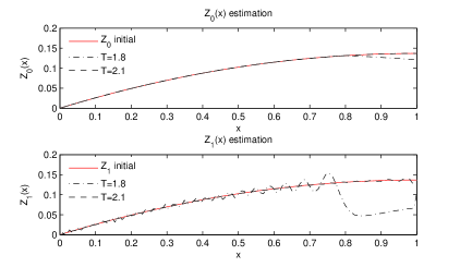
Figure 1: Initial condition recovery after $10$ iterations

Table 2: Computation time for $10$ iterations

T	Computation time (sec)
2.10	3.0469
3.00	3.6875
5.00	4.2813
10.00	5.9219

5 Conclusions

The LMI approach to observers and initial state recovering of semilinear N-D wave equations on a hypercube has been presented. In the linear 2-D case our results lead to an upper bound on the exact observability time, which is close to the analytical value, but does not recover it as it happened in 1-D case. For 1-D systems with locally Lipschitz nonlinearities we have found a (lower) bound on the region of initial values that are uniquely recovered from the measurements on the finite interval.

References

- [1] K. Ammari, S. Nicaise, and C. Pignotti. Feedback boundary stabilization of wave equations with interior delay. Systems & Control Letters, 59(10):623–628, 2010.
- [2] M. Baroun, B. Jacob, L. Maniar, and R. Schnaubelt. Semilinear observation systems. Systems & Control Letters, 62, 2013.
- [3] S. Boyd, L. El Ghaoui, E. Feron, and V. Balakrishnan. Linear Matrix Inequality in Systems and Control Theory. SIAM Frontier Series, 1994.
- [4] F. Castillo, E. Witrant, C. Prieur, and L. Dugard. Dynamic boundary stabilization of linear and quasi-linear hyperbolic systems. In IEEE 51st Conference on Decision and Control, pages 2952–2957, 2012.
- [5] E. Fridman. Observers and initial state recovering for a class of hyperbolic systems via Lyapunov method. Automatica, 49(7):2250–2260, 2013.
- [6] E. Fridman, S. Nicaise, and J. Valein. Stabilization of second order evolution equations with unbounded feedback with time-dependent delay. SIAM Journal on Control and Optimization, 48(8):5028–5052, 2010.
- [7] E. Fridman and Y. Orlov. Exponential stability of linear distributed parameter systems with time-varying delays. Automatica, 45(2):194–201, 2009.
- [8] E. Fridman and Y. Orlov. An LMI approach to boundary control of semilinear parabolic and hyperbolic systems. Automatica, 45(9):2060–2066, 2009.
- [9] B.-Z. Guo, H.-C. Zhou, and C.-Z. Yao. The stabilization of multi-dimensional wave equation with boundary control matched disturbance. In IFAC World Congress, Cape Town, 2014.
- [10] G. H. Hardy, J. E. Littlewood, and G. Pólya. Inequalities. Mathematical Library, Cambridge, 1988.
- [11] H. K. Khalil. Nonlinear Systems. Prentice Hall, 3rd edition, 2002.
- [12] P.-O. Lamare, A. Girard, and C. Prieur. Lyapunov techniques for stabilization of switched linear systems of conservation laws. 2013.
- [13] J.-L. Lions. Exact controllability, stabilization and perturbations for distributed systems. SIAM review, 30(1):1–68, 1988.
- [14] A. Pazy. Semigroups of linear operators and applications to partial differential equations, volume 44. Springer New York, 1983.
- [15] K. Ramdani, M. Tucsnak, and G. Weiss. Recovering the initial state of an infinite-dimensional system using observers. Automatica, 46(10):1616–1625, 2010.
- [16] M. Tucsnak and G. Weiss. Observation and control for operator semigroups. Springer, 2009.
- [17] V. Yakubovich. S-procedure in nonlinear control theory. Vestnik Leningrad University, 1:62–77, 1971.
- [18] E. Zuazua. Uniform stabilization of the wave equation by nonlinear boundary feedback. SIAM Journal on Control and Optimization, 28(2):466–477, 1990.