Application of an Extended Random Phase Approximation on Giant Resonances in Light, Medium and Heavy Mass Nuclei

Abstract

We present results of the time blocking approximation (TBA) on giant resonances in light, medium and heavy mass nuclei. The TBA is an extension of the widely used random-phase approximation (RPA) adding complex configurations by coupling to phonon excitations. A new method for handling the single-particle continuum is developed and applied in the present calculations. We investigate in detail the dependence of the numerical results on the size of the single particle space and the number of phonons as well as on nuclear matter properties. Our approach is self-consistent, based on an energy-density functional of Skyrme type where we used seven different parameter sets. The numerical results are compared with experimental data.

I Introduction

Self-consistent mean-field models have developed over the decades to a powerful tool for the description of nuclear structure and dynamics all over the periodic table Vretenar et al. (2005); Bender et al. (2003); Goriely et al. (2002); Kortelainen et al. (2010a). Time-dependent mean-field theory allows to simulate a great variety of excitations and dynamical processes Maruhn et al. (2014). Giant resonances are described well in the small amplitude limit where the space of one-particle one-hole $1p1h$ excitations is explored which is, in fact, identical to the widely used random phase approximation ( RPA). Here one is able to calculate mean energies and total transition strengths. In order to describe also the fine structure of bound states and the total width of giant resonances one has to include correlations beyond $1p1h$. Such calculations have been performed in self-consistent as well as in non-self-consistent approaches. Extended theories may include, e.g., two-particle two-hole configurations Drożdż et al. (1990) or one may consider the fragmentation of the single-particle states due to the coupling to phonons Dehesa et al. (1977); Tselyaev (1989, 2007); Lyutorovich et al. (2015). Within the latter approach isoscalar electric monopole resonances and quadrupole resonances were well reproduced in medium and heavy mass nuclei Kamerdzhiev et al. (1993, 2004); Litvinova and Tselyaev (2007); Tselyaev (2007); Lyutorovich et al. (2015). In light nuclei like ¹⁶O the present theory is unable to reproduce the experimental isoscalar cross sections quantitatively as important decay channels are still missing. This will be discussed in chapter III.

One might assume that mean-field theories which describe bulk properties of nuclei, such as the Thomas-Reiche-Kuhn (TRK) sum rule and the nuclear symmetry energy Berman and Fultz (1975), as well as shell effects rather well should also reproduce the centroid energies of the giant dipole resonance (GDR). This is not the case, however, as has worked out in systematic surveys based on RPA spectra Klüpfel et al. (2009); Erler et al. (2011, 2010). It was impossible to describe ground-state properties and the centroid energy of the GDR both in light and heavy nuclei with the same effective interaction. The problem is more serious than it might appear at a first glance because the physics of the GDR is closely connected with the neutron skin thickness and the low-lying dipole strength: the so-called pygmy resonances Abrahamyan et al. (2012); Tamii et al. (2011); Savran et al. (2011). These states are presently investigated experimentally because of their impact on the isotope abundance produced in supernova explosions Horowitz and Piekarewicz (2001).

Recently we showed that the explicit inclusion of quasi particle-phonon coupling may help to solve the problem of mean-field theories in reproducing the centroid energies of the GDRLyutorovich et al. (2012). Within the time blocking approximation (TBA) Tselyaev (1989, 2007), we obtained a reasonably good quantitative agreement with the experimental data for the GDR in light (¹⁶O), medium (⁴⁸Ca) and heavy (²⁰⁸Pb) nuclei. As we went beyond the mean-field approach we had to adjust new Skyrme forces, where we concentrated on the GDR in ¹⁶O within the conventional $1p1h$ RPA. The phonon contribution did hardly change the $1p1h$ RPA result in ¹⁶O but moved the GDR in ⁴⁸Ca and ²⁰⁸Pb closer to the experimental values. The isoscalar giant monopole (GMR) and giant quadrupole resonances (GQR) were shown in a short note Lyutorovich et al. (2015) using an improved version of TBA that derived all matrix elements consistently from the given (Skyrme) energy-density functional and calculated them without any approximations and included the single-particle continuum thus avoiding the artificial discretization implied in earlier TBA calculations. The present publication discusses in detail the formalism of the short note Lyutorovich et al. (2015). Moreover, we present a new treatment of the single-particle continuum which allows to include exactly the velocity dependent terms and the spin-orbit interaction. We scrutinize the phonon-coupling model by studying the dependence of the results on the numerical parameters of the model (more formal details were presented recently in Lyutorovich et al. (2016)). The theoretical spectral distributions for the GMR, GQR and GDR of ¹⁶O, ⁴⁰Ca, ⁴⁸Ca and ²⁰⁸Pb are compared with the experimental ones. We use seven different Skyrme parametrizations in order to find out how these giant resonances depend on some specific gross properties of nuclear matter. As an important result we found that the isoscalar GMR and GQR as well as isovector GDR can be simultaneously well reproduced by properly chosen Skyrme parametrizations.

The paper is organized as follows. In Chapter II we present in the Sec. A the basic formulas of the self-consistent RPA and TBA. In Sec. B we present seven different Skyrme parametrizations which reproduce the usual ground-state properties and give reasonably good results for isovector as well as isoscalar electric giant resonances. The Skyrme parametrizations were characterized in terms of nuclear matter properties (NMP) from which we consider in particular four key quantities: incompressibility $K$, effective mass $m^{*}/m$, symmetry energy, and enhancement factor for the TRK sum rule $\kappa_{\mathrm{TRK}}$ (equivalent to isovector effective mass). We investigated in detail the influence of these four NMP on the GDR, the giant isoscalar monopole and quadrupole resonances. Problems connected with the tuning of the parameters are discussed in Sec. C. Details of the calculation scheme are given in Chapter III. In Sec. A we discuss the single-particle basis and in Sec. B the effect of the exact continuum treatment on our results. In Sec. C we investigate in detail the dependence of the TBA results on the number of phonons included. Chapter IV presents our results. In Sec. A the impact of the phonon coupling on the resonances is shown and in Sec. B we compare our final results with experimental data. In the last chapter we summarize our investigations.

II The method

II.1 The basic equations

II.1.1 Conventional RPA

The original derivation of the RPA equations in nuclear physics is based on the time-dependent Hartree-Fock methods where one considered small amplitude dynamics about a Hartree-Fock ground state Brown (1971). From this derivation, one may obtain the impression that the RPA is a very limited approach. This is actually not the case if one considers the derivation within the Green function method. All details and the explicit expressions can be found in Ref. Speth et al. (1977). The transition matrix element of a one-particle operator between the exact ground state of an $A$-particle system and an excited state $m$ is given as:

$$\langle Am|Q|A0\rangle\;=\sum_{\nu_{1}\nu_{2}}Q^{\rm eff}_{\nu_{1}\nu_{2}}\;\chi^{m}_{\nu_{1}\nu_{2}}.$$ (1)

Here Q^eff are effective operators and $\chi^{m}$ are the quasiparticle-quasihole matrix elements which are given by the equation:

$$\left(\epsilon_{\nu_{1}}-\epsilon_{\nu_{2}}-\Omega\right)\chi^{m}_{\nu_{1}\nu_{2}}=$$

$$\left(n_{\nu_{1}}-n_{\nu_{2}}\right)\sum_{\nu_{3}\nu_{4}}F^{ph}_{\nu_{1}\nu_{4}\nu_{2}\nu_{3}}\;\chi^{m}_{\nu_{3}\nu_{4}}$$ (2)

where F^ph is the renormalized $ph$ interaction. All relations have been been derived without any approximations. Therefore conservation laws can be applied. E.g., the effective electric operators reduces to the bare ones due to Ward identities in the long-wave length limit. The derivation of the RPA equation starts with the equation of motion (Dyson equation) for the one-particle Green function. The basic input is the mass operator $\Sigma$ which include all information on the many-body system. The most general form is given as:

$$\Sigma=\Sigma{(\mathbf{r},\mathbf{p},\epsilon)}$$ (3)

It depends on the coordinate $\mathbf{r}$, the momentum $\mathbf{p}$ (non-locality), and the energy $\epsilon$.

Note: the RPA equations derived here are formally identical with the corresponding equations derived in the linear response limit of time-dependent density-functional theory (TDDFT) in the next section. The crucial difference is the mass operator in Eq. 3 which is energy dependent in a general many-body theory whereas it turns out to be independent of energy in (TDDFT). As the various quantities in the general case and in linear response are different, we also use different symbols.

In the general case, the expression for the effective mass has the form:

$$\frac{m}{m^{*}}=\frac{\left(1+2m\frac{\delta\Sigma}{\delta p^{2}}\right)_{F}}{\left({1-\frac{\delta\Sigma}{\delta\epsilon}}\right)_{F}}.$$ (4)

The nominator is called $k$-mass and the denominator $E$-mass Jeukenne et al. (1976). They are related to the non-locality and energy-dependence of the mass operator, respectively. If the mass operator does not depend on the energy, the denominator is equal to one. In the case of a totally energy independent mass operator, the formulas become much simpler as the single-particle strength is equal to one Grümmer and Speth (2006). The effective operators are in all cases equal to the bare operators and also the $ph$-interaction is not renormalized.

In our extended model (the TBA), we introduce complex configurations by coupling phonons to the single-particle states. This introduces an energy dependence into the mass operator in first order Wambach et al. (1982). For this reason the single-particle strength is less then one and we obtain a contribution to the $E$-mass. This is the well known shift due to phonon coupling. All this is correctly taken care of in the TBA. But we will not address single-particle effects explicitely later on.

II.1.2 Self-consistent RPA

Our approach is based on the version of the response function formalism developed within the Green function method (see Ref. Speth et al. (1977)). In the general case the distribution of the strength of transitions in the nucleus caused by some external field represented by the single-particle operator $Q$ is determined by the strength function $S(E)$ which is defined in terms of the response function $R(\omega)$ by the formulas

$$S(E)=-\frac{1}{\pi}\;\mbox{Im}\,\Pi(E+i\Delta)\,,$$ (5)

$$\Pi(\omega)=-\langle\,Q\,|\,R(\omega)\,|\,Q\,\rangle\,,$$ (6)

where $E$ is an excitation energy, $\Delta$ is a smearing parameter, and $\Pi(\omega)$ is the (dynamic) polarizability.

The first model used in our calculations is the self-consistent RPA based on TDDFT with the energy density functional $E[\rho]$. The TDDFT equations imply that $[\,\rho,h\,]=0$ where $\rho$ is the single-particle density matrix satisfying the condition $\rho^{2}=\rho$, and $h$ is the single-particle Hamiltonian,

$$h^{\vphantom{*}}_{12}=\frac{\delta E[\rho]}{\delta\rho^{\vphantom{*}}_{21}}\,.$$ (7)

The numerical indices here and in the following denote the set of the quantum numbers of some single-particle basis. It is convenient to introduce the basis that diagonalizes simultaneously the operators $h$ and $\rho\,$:

$$h^{\vphantom{*}}_{12}=\varepsilon^{\vphantom{*}}_{1}\delta^{\vphantom{*}}_{12}\,,\qquad\rho^{\vphantom{*}}_{12}=n^{\vphantom{*}}_{1}\delta^{\vphantom{*}}_{12}\,,$$ (8)

where $n^{\vphantom{*}}_{1}=0,1$ is the occupation number. In what follows the indices $p$ and $h$ will be used to label the single-particle states of the particles ($n^{\vphantom{*}}_{p}=0$) and holes ($n^{\vphantom{*}}_{h}=1$) in this basis.

In RPA, the response function is a solution of the following Bethe-Salpeter equation (BSE)

$$R^{{}_{\mbox{\scriptsize RPA}}}_{\vphantom{1}}(\omega)=R^{(0)}_{\vphantom{1}}(\omega)-R^{(0)}_{\vphantom{1}}(\omega)VR^{{}_{\mbox{\scriptsize RPA}}}_{\vphantom{1}}(\omega)\,,$$ (9)

where $R^{(0)}_{\vphantom{1}}(\omega)$ is the uncorrelated $1p1h$ propagator and $V$ is the residual interaction. The $1p1h$ propagator $R^{(0)}_{\vphantom{1}}(\omega)$ is defined as

$$R^{(0)}_{\vphantom{1}}(\omega)=-\bigl{(}\,\omega-\Omega^{(0)}_{\vphantom{1}}\bigr{)}^{-1}M^{{}_{\mbox{\scriptsize RPA}}}_{\vphantom{1}},$$ (10)

where the matrices $\Omega^{(0)}_{\vphantom{1}}$ and $M^{{}_{\mbox{\scriptsize RPA}}}_{\vphantom{1}}$ are defined in the $1p1h$ configuration space. $M^{{}_{\mbox{\scriptsize RPA}}}_{\vphantom{1}}$ is the metric matrix

$$M^{{}_{\mbox{\scriptsize RPA}}}_{12,34}=\delta^{\vphantom{*}}_{13}\,\rho^{\vphantom{*}}_{42}-\rho^{\vphantom{*}}_{13}\,\delta^{\vphantom{*}}_{42}\,.$$ (11)

The matrix $\Omega^{(0)}_{\vphantom{1}}$ has the form

$$\Omega^{(0)}_{12,34}=h^{\vphantom{*}}_{13}\,\delta^{\vphantom{*}}_{42}-\delta^{\vphantom{*}}_{13}\,h^{\vphantom{*}}_{42}\,.$$ (12)

In the self-consistent RPA based on the energy density functional $E[\rho]$ one has

$${V}^{\vphantom{*}}_{12,34}=\frac{\delta^{2}E[\rho]}{\delta\rho^{\vphantom{*}}_{21}\,\delta\rho^{\vphantom{*}}_{34}}\,,$$ (13)

so the quantities $h$ and $V$ appear to be linked by Eqs. (7) and (13).

The propagator $R^{{}_{\mbox{\scriptsize RPA}}}_{\vphantom{1}}(\omega)$, being a matrix in $1p1h$ space, is a rather bulky object. For practical calculations, it is more convenient to express it in terms of RPA amplitudes $z_{12}^{n}$ by virtue of the spectral representation

$$R^{{}_{\mbox{\scriptsize RPA}}}_{1234}(\omega)=-\sum_{n}z_{12}^{n}\frac{\mbox{sgn}(\omega_{n})}{\omega-\omega_{n}}(z_{34}^{n})^{*}$$ (14)

where $n$ labels the RPA eigenmodes and $\omega_{n}$ is the eigenfrequency. Inserting that into Eq. (9) and filtering the pole at $\omega=\omega_{n}$ yields the familiar RPA equations

$$\sum_{34}\left(\Omega^{(0)}_{12,34}+\sum_{56}M^{{}_{\mbox{\scriptsize RPA}}}_{12,56}\,{V}^{\vphantom{*}}_{56,34}\right)\,z^{n}_{34}=\omega^{\vphantom{*}}_{n}\,z^{n}_{12}\,,$$ (15)

where the transition amplitudes ${z}^{n}$ are normalized by the condition

$$\sum_{12,34}({z}^{n}_{12})^{*}\,M^{{}_{\mbox{\scriptsize RPA}}}_{1234}\,{z}^{n^{\prime}}_{34}=\mbox{sgn}(\omega^{\vphantom{*}}_{n})\,\delta^{\vphantom{*}}_{n,\,n^{\prime}}.$$ (16)

These equations determine the set of eigenstates $n$ with amplitudes $z^{n}_{12}$ and frequencies $\omega_{n}$.

II.1.3 Phonon coupling model

The second model is the quasiparticle-phonon coupling model within the time-blocking approximation (TBA) Tselyaev (1989); Kamerdzhiev et al. (1997, 2004); Tselyaev (2007) (without ground state correlations beyond the RPA included in Tselyaev (1989); Kamerdzhiev et al. (1997, 2004); Tselyaev (2007) and without pairing correlations included in Tselyaev (2007)). This model, which in the following will be referred to as TBA, is an extension of RPA including $1p1h\otimes$phonon configurations in addition to the $1p1h$ configurations incorporated in the conventional RPA. The BSE for the response function in the TBA is

$$R^{{}_{\mbox{\scriptsize TBA}}}_{\vphantom{1}}(\omega) = R^{(0)}_{\vphantom{1}}(\omega)$$ (17)

$$-R^{(0)}_{\vphantom{1}}(\omega)(V\!+\!\tilde{W}(\omega))R^{{}_{\mbox{\scriptsize TBA}}}_{\vphantom{1}}(\omega)\,,$$

$$\tilde{W}(\omega) = W(\omega)-{W}(0)\,,$$ (18)

where the induced interaction $\tilde{W}(\omega)$ serves to include contributions of $1p1h\otimes$phonon configurations.

The matrix ${W}(\omega)$ in Eq. (18) is defined in the $1p1h$ subspace and can be represented in the form

$${W}^{\vphantom{*}}_{12,34}(\omega)=\sum_{c,\;\sigma}\,\frac{\sigma\,{F}^{c(\sigma)}_{12}{F}^{c(\sigma)*}_{34}}{\omega-\sigma\,\Omega^{\vphantom{*}}_{c}}\,,$$ (19)

where $\sigma=\pm 1$, $\,c=\{p^{\prime},h^{\prime},n\}$ is an index of the subspace of $1p1h\otimes$phonon configurations, $n$ is the phonon’s index,

$$\Omega^{\vphantom{*}}_{c}=\varepsilon^{\vphantom{*}}_{p^{\prime}}-\varepsilon^{\vphantom{*}}_{h^{\prime}}+\omega^{\vphantom{*}}_{n}\,,\quad\omega^{\vphantom{*}}_{n}>0\,,$$ (20)

$${F}^{c(-)}_{12}={F}^{c(+)*}_{21},\qquad{F}^{c(-)}_{ph}={F}^{c(+)}_{hp}=0\,,$$ (21)

$${F}^{c(+)}_{ph}=\delta^{\vphantom{*}}_{pp^{\prime}}\,g^{n}_{h^{\prime}h}-\delta^{\vphantom{*}}_{h^{\prime}h}\,g^{n}_{pp^{\prime}},$$ (22)

$g^{n}_{12}$ is an amplitude of the quasiparticle-phonon interaction. These $g$ amplitudes (along with the phonon’s energies $\omega^{\vphantom{*}}_{n}$) are determined by the positive frequency solutions of the RPA equations and the emerging $z$ amplitudes as

$$g^{n}_{12}=\sum_{34}{V}^{\vphantom{*}}_{12,34}\,z^{n}_{34}\,.$$ (23)

where $V_{12,34}$ is the same residual interaction (13) as used in RPA. In our DFT-based approach the energy density functional $E[\rho]$ in Eqs. (7) and (13) is the functional of the Skyrme type with free parameters which are adjusted to experimental data. In this case $E[\rho]$ already effectively contains a part (actually the stationary part) of the contributions of those $1p1h\otimes$phonon configurations which are explicitly included in the TBA. Therefore, in the theory going beyond the RPA, the problem of double counting and of ground-state stability arises Toepffer and Reinhard (1988). To avoid this problem in the TBA, we use the subtraction method. It consists in the replacement of the amplitude ${W}(\omega)$ by the quantity $\bar{W}(\omega)={W}(\omega)-{W}(0)$ as it is given in Eq. (17). In Ref. Tselyaev (2013) it was shown that, in addition to the elimination of double counting, the subtraction method ensures stability of solutions of the TBA eigenvalue equations.

II.2 Basics on the Skyrme functional and related parameters

From the variety of self-consistent nuclear mean-field models Bender et al. (2003), we consider here a non-relativistic branch, the widely used and very successful Skyrme-Hartree-Fock (SHF) functional. A detailed description of the functional is found in the reviews Bender et al. (2003); Stone and Reinhard (2007); Erler et al. (2011). We summarize the essential features: The functional depends on a couple of local densities and currents (density, gradient of density, kinetic-energy density, spin-orbit density, current, spin density, kinetic spin-density). It consists of quadratic combinations of these local quantities, corresponding to pairwise contact interactions. The term with the local densities is augmented by a non-quadratic density dependence to provide appropriate saturation. One adds a simple pairing functional to account for nuclear superfluidity. The typically 13–14 model parameters are determined by a fit to a large body of experimental data on bulk properties of the nuclear ground state. For recent examples see Goriely et al. (2002); Klüpfel et al. (2009); Kortelainen et al. (2010b).

The properties of the forces can be characterized, to a large extend, by nuclear matter properties (NMP), i.e. equilibrium properties of homogeneous, symmetric nuclear matter, for which we have some intuition from the liquid-drop model Myers (1977). Of particular interest for resonance excitations are the NMP which are related to response to perturbations: incompressibility $K$ (isoscalar static), effective mass $m^{*}/m$ (isoscalar dynamic), symmetry energy $a_{\mathrm{sym}}$ (isovector static), TRK sum rule enhancement $\kappa_{\mathrm{TRK}}$ (isovector dynamic). We aim at exploring the effect of phonon coupling under varying conditions and thus use here parametrizations from recent fits presented in Klüpfel et al. (2009) which provides a systematic variation of these four NMP.

	$K$ [MeV]	$m^{*}/m$	$a_{\mathrm{sym}}$ [MeV]	$\kappa_{\mathrm{TRK}}$
SV-bas	234	0.90	30	0.4
SV-kap00	234	0.90	30	0.0
SV-mas07	234	0.70	30	0.4
SV-sym34	234	0.90	34	0.4
SV-K218	218	0.90	30	0.4
SV-m64k6	241	0.64	27	0.6
SV-m56k6	255	0.56	27	0.6

Table 1: Nuclear matter properties for the Skyrme paramterizations used in this study: incompressibility $K$, isoscalar effective mass $m^{*}/m$, symmetry energy $a_{\mathrm{sym}}$, Thomas-Reiche-Kuhn sum rule enhancement $\kappa_{\mathrm{TRK}}$. The first five parametrizations stem from Klüpfel et al. (2009), the last two from Lyutorovich et al. (2012).

Table 1 lists the selection of parametrizations and their NMP. SV-bas is the base point of the variation of forces. Its NMP are chosen such that dipole polarizability and the three most important giant resonances (GMR, GDR, and GQR) in ²⁰⁸Pb are well reproduced by Skyrme-RPA calculations. Each one of the next four parametrizations vary exactly one NMP while keeping the other three at the SV-bas value. These 1+4 parametrizations allow to explore the effect of each NMP separately. It was figured out in Klüpfel et al. (2009) that there is a strong relation between each one of the four NMP and one specific giant resonance: $K$ affects mainly the GMR, $m^{*}/m$ affects mainly the GQR, $\kappa_{\mathrm{TRK}}$ affects the GDR, and $a_{\mathrm{sym}}$ is linked to the dipole polarizability Nazarewicz et al. (2014).

Finally, the last two parametrizations in Table 1 were developed in Lyutorovich et al. (2012) with the goal to describe, within TBA, at the same time the GDR in ¹⁶O and ²⁰⁸Pb. This required to push up the RPA peak energy which was achieved by low $a_{\mathrm{sym}}$ in combination with high $\kappa_{\mathrm{TRK}}$. To avoid unphysical spectral distributions for the GDR, a very low $m^{*}/m$ was used.

II.3 The problem of tuning a parametrization

Looking only on average resonance energies, the tuning of parametrizations is simple. As mentioned before, the three giant resonances which we consider couple each one almost exclusively to one property, the GMR to the incompressibility $K$, the GDR to the TRK sum rule enhancement $\kappa_{\mathrm{TRK}}$, and the GQR to the isoscalar effective mass $m^{*}/m$. This suggests that one can adjust these three resonances independently at wish. However, problems appear when looking at the detailed spectral distributions. We observed in our investigations that the shift in average resonance energies does usually not correspond to a global shift of the spectral distribution, but rather to a redistribution of strength over the spectrum. However, such redistribution can lead to unrealistic profiles and that is what is often hindering a light-hearted adjustment.

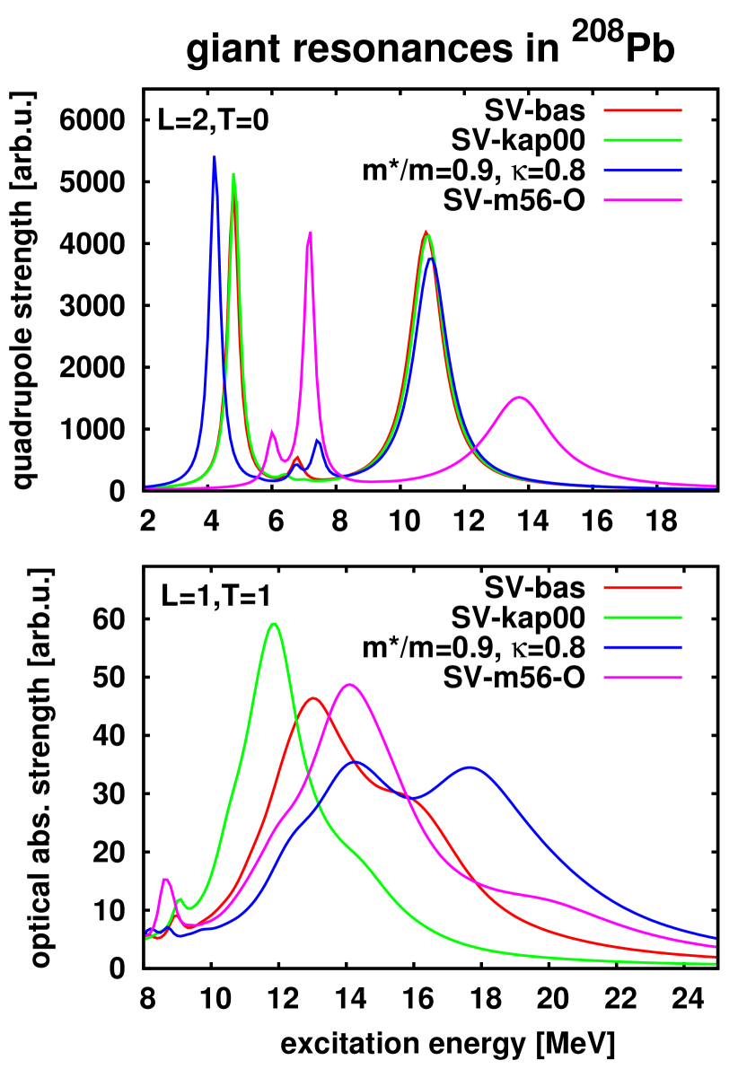
Figure 1: Dipole strength (lower panel) and quadrupole strength (upper panel) for four parametrizations as indicated. The smooth spectra are obtained from folding with Gaussians of linearly increasing width $\Gamma=\mbox{max}(0.2,(E-8)/5)$ MeV.

Figure 1 shows detailed spectra for four parametrizations. SV-kap00 as compared to SV-bas corresponds to a shift of $\kappa_{\mathrm{TRK}}$ from 0.4 (for SV-bas) down to 0. This has no effect on the GQR and leads to a visible downshift of the GDR. This downshift does also change the profile to the extend that high-energy bump at 16 MeV in SV-bas now appears at 14 MeV and, more important, becomes much smaller. Thus the way from SV-kap00 to SV-bas already changes somewhat the profile, but at a harmless level.

Now we try to up-shift the GDR by enhancing dramatically $\kappa_{\mathrm{TRK}}$ to 0.8 while keeping $m^{*}/m=0.9$ at the value of SV-bas. This leads to the blue curves in the figure. It is gratifying to see that the GQR remains where it should be. The GDR makes the wanted up-shift. However, this happens at the price of a totally unrealistic double humped structure of the GDR. Mind that the upper bump appears in so pronounced manner in spite of energy-dependent folding width. Mere enhancement of $\kappa_{\mathrm{TRK}}$ seems thus no solution to the wanted up-shift of the GDR. The former solution was to use much lower $m^{*}/m=0.56$ to curb down the double hump. This is successful for the GDR (purple line) however disastrous for the GQR. Not only that the too high GQR position cannot be cured by phonon coupling, but also that the low energy spectrum is grossly unrealistic. This looks like a deadlock for global improvment and it is at the level of RPA. The situation becomes more gracefull for TBA as we will see later.

III Details of the calculation scheme

III.1 Single-particle basis and residual interaction

The response functions both for RPA and TBA, Eqs. (9) and (17), are solved in a discrete basis defined as a set of solutions of the Schrödinger equation with box boundary conditions. Both equations are solved in the same large configuration space. A new method to include the continuum in the discrete basis representation is explained in Appendix A. The residual interaction $V$ in Eqs.(9) and (17) is derived from the energy functionals according to Eq. (13). In the case of the energy density functional $E[\rho]$ built on the Skyrme forces, the amplitude $V$ determined by Eq. (13) contains zero-range (velocity-independent) and velocity-dependent parts. The scheme for taking into account the zero-range part of the residual interaction adopted in our calculations is described in Refs. Litvinova and Tselyaev (2007); Tselyaev (2007). A detailed description of the computation of the matrix elements in connection with the Skyrme functional is found in Lyutorovich et al. (2016).

We will consider only doubly-magic nuclei. They have closed shells and pairing is inactive. The box sizes in the RPA and TBA calculations are 15 fm for ¹⁶O, ^40,48Ca and 18 fm for ²⁰⁸ Pb. The single-particle basis in which we solve the RPA and TBA equations include single-particle states up to $\varepsilon_{\text{max}}$ = 100 MeV (see our discussion in the next two sections). In the TBA calculations we apply the subtraction recipe (18) Tselyaev (2013). As mentioned before, this procedure eliminates double counting, resolves stability problems, and restores the Thouless theorem.

III.2 Effect of the exact Continuum

As mentioned before, we included the full single-particle continuum into our TBA calculations. For this, we use a new technique which allows a continuum treatment in connection with full self-consistency RPA as outlined in Appendix A. This method uses the discrete basis representation and recovers the exact method Shlomo and Bertsch (1975) of treatment of the continuum in the coordinate representation if the discrete basis is sufficiently complete ($\varepsilon_{\text{max}}$ high enough) and the radius of the box ($R_{\mbox{\scriptsize box}}$) is sufficiently large (see Appendix A). To check the accuracy of our method, we first compare the results obtained within the continuum RPA (CRPA) in the discrete basis representation (hereafter called CRPA${}_{\,\mbox{\scriptsize d.b.}}$) with the results of the CRPA in the coordinate representation (CRPA${}_{\,\mbox{\scriptsize c.r.}}$). As an example, we consider calculations of the GMR in the fully self-consistent CRPA based on the Skyrme energy density functional with the T6 parametrization Tondeur et al. (1984) producing the nucleon effective mass $m^{*}/m=1$. As was shown in Ref. Tselyaev et al. (2009), the fully self-consistent CRPA${}_{\,\mbox{\scriptsize c.r.}}$ scheme in this special case has relatively simple form. The results for the nucleus ¹⁶O are shown in Fig. 2. The function $F(E)$ presented in this figure is the fraction of the energy-weighted sum rule (EWSR) defined as

$$F(E)=E\,S(E)/m_{1}\,,$$ (24)

where $S(E)$ is the strength function defined in Eq.(5) and $m_{1}=\int dE,\,E\,S(E)$ is the energy-weighted moment of $S(E)$ determined by the known EWSR Bohigas et al. (1979).

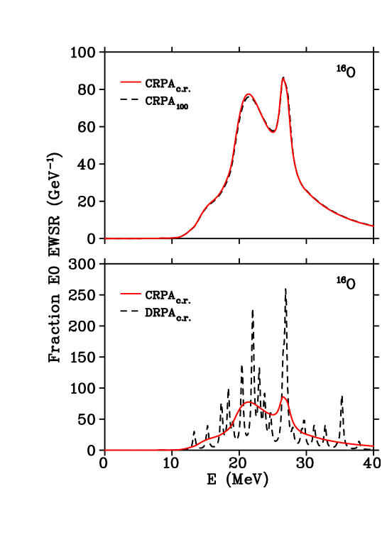
Figure 2: ISGMR in ¹⁶O calculated within fully self-consistent RPA based on the Skyrme energy density functional with the T6 parametrization Tondeur et al. (1984). Fractions of the $E0$ EWSR are shown. Upper panel: the CRPA${}_{\,\mbox{\scriptsize c.r.}}$ function obtained by making use of the method of Ref. Tselyaev et al. (2009) is presented by the red solid line. The CRPA${}_{\,\mbox{\scriptsize 100}}$ function obtained in the discrete basis with $\varepsilon_{\text{max}}$ = 100 MeV is presented by the black dashed line. Lower panel: the CRPA${}_{\,\mbox{\scriptsize c.r.}}$ function (red solid line) is compared with the DRPA${}_{\,\mbox{\scriptsize c.r.}}$ function (black dashed line) obtained by the same method of Ref. Tselyaev et al. (2009). Smearing parameter $\Delta$ = 200 keV was used in all the calculations.

In the upper panel of Fig. 2 the CRPA${}_{\,\mbox{\scriptsize c.r.}}$ results are compared with CRPA${}_{\,\mbox{\scriptsize 100}}$ obtained in the discrete basis with $E_{\mbox{\scriptsize cut}}$ = 100 MeV. The equations of the CRPA${}_{\,\mbox{\scriptsize c.r.}}$ were solved with a mesh spacing $h=0.05$ fm in $r$-space and box size $R_{\mbox{\scriptsize box}}=15$ fm. All these calculations used a smearing parameter $\Delta$ = 200 keV. The difference between the CRPA₁₀₀ and CRPA${}_{\,\mbox{\scriptsize c.r.}}$ curves is small and hardly visible.The CRPA₃₀₀ obtained in the discrete basis with $E_{\mbox{\scriptsize cut}}$ = 300 MeV and CRPA${}_{\,\mbox{\scriptsize c.r.}}$ curves are practically indistinguishable, so we do not show them. In the lower panel of Fig. 2 the discrete RPA (DRPA) results obtained by the coordinate representation method of Ref. Tselyaev et al. (2009) are compared with the CRPA function for ¹⁶O and, again, $\Delta$ = 200 keV. In this case, the difference between these results is large.

Thus we see that the magnitude of the continuum effects on nuclear excitations is different in light and heavy nuclei. To see the trend we have calculated the GDR in the nuclei ¹⁶O, ⁴⁸Ca, ¹³²Sn and ²⁰⁸Pb within two schemes: CRPA${}_{\,\mbox{\scriptsize d.b.}}$ and DRPA${}_{\,\mbox{\scriptsize d.b.}}$ using the Skyrme parametrization SV-bas Klüpfel et al. (2008). The results are presented in Fig. 3. In this figure, the photo-absorption cross sections normalized to the classical values $\sigma_{\mbox{\scriptsize class.}}=\frac{5}{3}\pi\langle r^{2}\rangle$ are shown. The mean-square radii $\langle r^{2}\rangle$ have been calculated for the each nucleus using its Skyrme-Hartree-Fock ground-state. The $\sigma_{\mbox{\scriptsize class.}}$ are: 378.5 mb for ¹⁶O, 654.5 mb for ⁴⁸Ca, 1204.0 mb for ¹³²Sn, and 1605.1 mb for ²⁰⁸Pb. As can be seen, the effect of the single-particle continuum is strongest in the light nuclei ¹⁶O and ⁴⁰Ca. In ¹⁶O nucleus, the CRPA and DRPA results significantly differ at $\Delta\lesssim$ 400 keV. Even at $\Delta=$ 1 MeV the difference is noticeable. It disappears only at $\Delta=$ 2 MeV. In ⁴⁸Ca the difference between the CRPA and DRPA becomes small at $\Delta\gtrsim$ 1 MeV. The same is true for ¹³²Sn, though in whole this difference here is less than in ⁴⁸Ca. These results are in agreement with the conclusions of Refs. Dehesa et al. (1977); Nakatsukasa and Yabana (2005); De Donno et al. (2011). In the heavy nucleus ²⁰⁸Pb, the effect of the single-particle continuum is small and is manifested only at $\Delta\lesssim$ 200 keV.

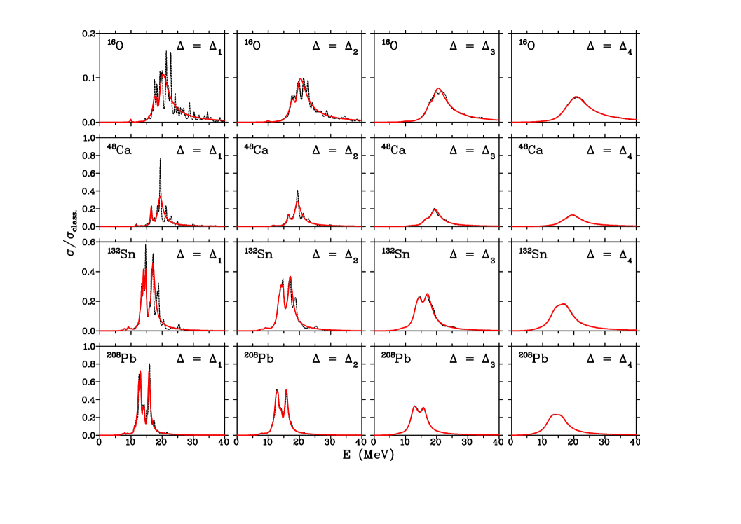
Figure 3: (Color online.) Photo-absorption cross sections in the nuclei ¹⁶O, ⁴⁸Ca, ¹³²Sn, and ²⁰⁸Pb calculated within the CRPA (red solid lines) and the DRPA (black dashed lines) with different smearing parameters $\Delta$: $\Delta_{1}=200$ keV, $\Delta_{2}=400$ keV, $\Delta_{3}=1$ MeV, and $\Delta_{4}=2$ MeV. The discrete basis representation with $E_{\mbox{\scriptsize cut}}=100$ MeV is used both in the CRPA and the DRPA. The calculated cross sections have been normalized to the classical values $\sigma_{\mbox{\scriptsize class.}}=\frac{5}{3}\pi\langle r^{2}\rangle$ (see text for more details). The results are obtained with the SV-bas Skyrme force parametrization Klüpfel et al. (2008).

In Fig. 4, for ¹⁶O, and Fig. 5, for ⁴⁰Ca, we compare the TBA results obtained with the exact continuum treatment (CTBA) and the discretized approximation (DTBA). Here, blue dashed and red dashed-dotted lines represent the DTBA results for smearing parameters $\Delta$ = 400 and 700 keV, respectively. The expression ”strength” in the Y-axes mean fractions EWSR for GMR and GQR and photo-absorption cross section for GDR. The experimental data for GMR and GQR in ¹⁶O were taken from Ref. Lui et al. (2001) and for GDR in ¹⁶O from Ishkhanov et al. (2002). The data for ⁴⁰Ca were taken from Refs. Anders et al. (2013) and Erokhova et al. (2003), respectively. The figures show that, for light nuclei, increasing $\Delta(\mbox{DTBA})$ damps the artificial fine structure of the discrete approach. But, at the same time, it wipes out important physical features. Hence, it is impossible to reproduce CTBA results for strength functions of light nuclei by using the DTBA, both with small and large smearing parameters.

The experimental profiles for the two isoscalar resonances in ¹⁶O look very different from the isovector GDR and from all resonances in heavier nuclei. The theoretical GQR shows a narrow peak where as the experimental strength is nearly continuously distributed over more then 20 MeV. The same is true also for the experimental GMR strength. Here the theoretical strength distribution is very broad and shows at least some qualitative similarity. There are little differences between the various parameter sets. The question arises why are we not able to reproduce theoretically these two resonances while the results in the heavier nuclei are in good qualitative in many cases even in quantitative agreement with experiment? For the GQR the explanation is simple: The dominant decay channel of the GQR in ¹⁶O is the $\alpha$-decay into the ground state and the first excited state of ¹²C Knöpfle et al. (1978).

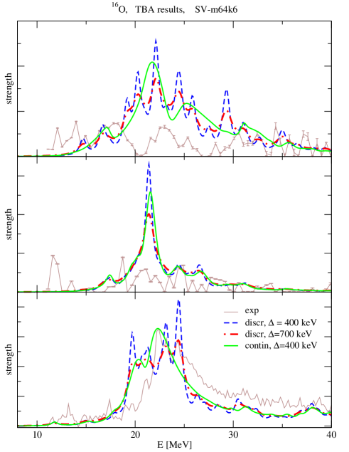
Figure 4: Discrete and continuum TBA results for ¹⁶O which were obtained with the parameter set SV-m64k6. The fractions EWSR for GMR and GQR and photo-absorption cross section for GDR are presented in the upper, middle and lower panel, respectively. The DTBA for smearing parameters $\Delta$ = 400 and 700 keV are given by blue dashed and red dashed-doted lines, respectively. Thick green and thin brown full lines represent CTBA with $\Delta$ = 400 keV and experimental data, respectively. The data are taken from Ref. Ishkhanov et al. (2002); Lui et al. (2001)

In the range between 18-23 MeV the $\alpha$-decay width is $90\%$ of the total decay width and between 23-27 MeV $70\%$. This reaction mechanism is included neither in RPA nor in TBA. This is probably the reason why theory overestimates the peak height of the cross section and does not reproduce the very broad experimental distribution. While the theoretical GQR cross section in ¹⁶O shows a well concentrated resonance, the theoretical monopole distribution is very broad as no narrow single-particle resonances can contribute. It resembles more the experimental pattern but is at least a factor of two too high in the resonance region. The situation is completely different for the GDR. Our continuum calculation reproduces nearly quantitatively the shape and magnitude of the experimental distribution. The reason is that the GDR is dominated by the 1$\hbar\omega$ transitions which practically exhaust the TRK-sum rule. However, the peak of the distribution are typically 1 MeV too low for the present Skyrme parameterization.

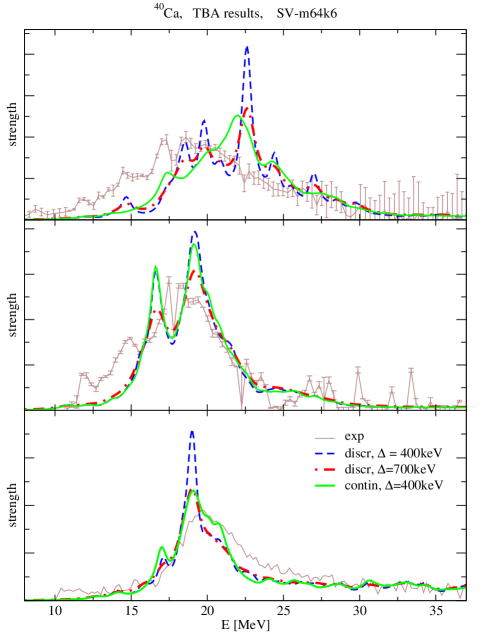
Figure 5: Same as in Fig. 4 but for ⁴⁰Ca. The corresponding data are taken from Ref. Erokhova et al. (2003); Anders et al. (2013)

Figure 5 compares DTBA and CTBA for the case of ⁴⁰Ca. The agreement between theory and experiment is very good for the GQR and GDR. In the case of the GMR our theoretical distribution is about 2 MeV too high compared with the experimental distribution.

III.3 The dependence on the number of phonons

In all the TBA calculations we use a large single-particle (s.p.) basis both in the phonons and in the complex ($1p1h\otimes$phonon) configurations, that is, a large number of $1p1h$ states in these configurations. As it was mentioned in Sec. III.1, the upper limit for s.p. energies in all calculations for all nuclei was $\varepsilon_{\text{max}}$ = 100 MeV. At the same time, only collective phonons were used in the complex configurations.

The dependence of the theoretical results on the number of phonons used in the calculation is of crucial importance. For this reason we investigate this question in some detail. The result of our investigations for the GDR in ¹⁶O is summarized in Fig. 6. The energies $E_{0}$ and the widths $\Gamma$ where derived from the theoretical cross section by a Lorentzian fit. We performed TBA calculations with and without the subtraction procedure. The two approaches give very different results. For comparison the RPA results are shown in the left upper corner of each figure.

In the left column of Fig. 6, the dependence of $E_{0}$ and $\Gamma$ is presented as a function of the maximal phonon energies $E^{\text{phon}}_{\text{max}}$. From Table 2, one obtains the connection between $E^{\text{phon}}_{\text{max}}$ and the number of phonons considered in each calculation. The single-particle basis in which we solve the RPA and TBA equations includes s.p. states up to $\varepsilon_{\text{max}}$ = 100 MeV and phonons up to the maximal phonon energy $E^{\text{phon}}_{\text{max}}$ = 80 MeV. In the right column the same quantities are shown as a function of the lower cutoff for transition strength $B_{\text{cut}}$ of the phonons where

$$B_{\text{cut}}=B(EL)/B(EL)_{\text{max}}\,,$$ (25)

$B(EL)_{\text{max}}$ is the maximal reduced probability of the excitation of the phonon states with the given angular momentum $L$. The connection between $B_{\text{cut}}$ and the number of phonons can be found again in Table 2. A too large number of phonons causes two problems: violation of the Pauli principle and double counting. We reduce these problems as we restrict ourselves in the actual calculations on phonons with $B_{\text{cut}}\geq 0.2$. Between $E^{\text{phon}}_{\text{max}}$ = 40 MeV and $E^{\text{phon}}_{\text{max}}$ = 80 MeV the energy and width remain stable if one applies the subtraction procedure. This corresponds 55 phonons and 66 phonons, respectively (see Table 2 and the text). In the right column the effect of an even larger number of phonons is presented. Here the transition strength parameter $B_{\text{cut}}$ ranges from 0.4 down 0.01. Here one sees strong changes only for the extreme cases of $B_{\text{cut}}$ = 0.05 and 0.01. The same is true also for the isoscalar resonances GMR and GQR as can be seen in Fig. 7. From this investigation we conclude that our results in ¹⁶O are stable for $\varepsilon_{\text{max}}$ = 100 MeV and 55 phonons.

Table 2: Relation between $E^{\text{phon}}_{\text{max}}$ and the number of phonons used in $1p1h\otimes$phonon configurations for ¹⁶O. The phonons were obtained in the $sp$ basis with $\varepsilon_{\text{max}}$ = 100 MeV and angular momenta up to $L_{\text{max}}=17$. Only collective phonons were used in our actual TBA calculations, that is, phonons with $B_{\text{cut}}\equiv B(EL)/B(EL)_{\text{max}}$ = 0.2 (see also the text). Under these conditions, the number of phonons is fixed by the maximum phonon energy $E^{\text{phon}}_{\text{max}}$. The effect of the noncollective phonons is demonstrated for small values $B_{\text{cut}}$ in the last two columns.

$B_{\text{cut}}$	0.4	0.3	0.2	0.2	0.2	0.2	0.2	0.1	0.05	0.01
$E^{\text{phon}}_{\text{max}}$	80	80	10	20	40	80	100	80	80	80
$N_{\text{phon}}$	42	52	1	6	55	66	69	117	166	325

Table 3: Dependence of the resonance energy and width (Lorentzian parameters $E_{0}$ and $\Gamma$) on the size of the sp basis used in phonons and in $1p1h\otimes$phonon configurations for ²⁰⁸Pb with $B_{\text{cut}}$ = 0.2. The size of the basis is characterized by the maximum energy $\varepsilon_{\text{max}}$.For the GDR, the parameters were calculated photoabsorption cross section while for GMR and GQR the fractions EWSR were used. All the values are given in MeV.

$\varepsilon_{\text{max}}$		50		100		150
$E^{\text{phon}}_{\text{max}}$	RPA	40		40		40
subtract.		no	yes	no	yes	no	yes
GDR $E_{0}$	15.0	13.5	14.4	13.3	14.3	13.3	14.3
$\Gamma$	4.60	4.63	4.57	4.61	4.53	4.63	4.54
GMR $E_{0}$	14.4	13.3	14.1	13.1	14.0	13.0	13.9
$\Gamma$	1.53	2.09	2.15	2.08	2.18	2.04	2.14
GQR $E_{0}$	12.8	11.1	11.9	10.9	11.8	10.8	11.7
$\Gamma$	1.04	1.10	1.13	1.10	1.19	1.10	1.24

In Table 3 we compare again TBA results obtained with and without the subtraction procedure as a function of the s.p. space. Here we used $B_{\text{cut}}$ = 0.2 which corresponds to 40 phonons. The results where the subtraction method was applied are very stable.

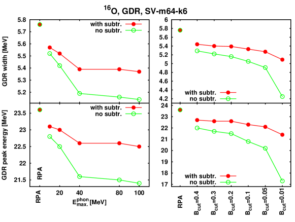
Figure 6: Energy (upper part) and width (lower part) of the GDR in ¹⁶O obtained from TBA calculations. The energy $E_{0}$ and the width $\Gamma$ are the corresponding parameters of a Lorentzian fit to the theoretical results. In the left corner of each figure the RPA result is given. In the left column we present $E_{0}$ and $\Gamma$ as a function of the maximal phonon energy $E^{\text{phon}}_{\text{max}}$ which we consider in each calculation. Table 2 gives the relation between energies and the number of phonons for $B_{cut}$=0.2. In the right column we present $E_{0}$ and $\Gamma$ as function of the minimal collectivity $B_{\text{cut}}$ of the phonons. The maximal phonon energy is in all cases $E^{\text{phon}}_{\text{max}}$ = 80 MeV.

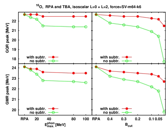
Figure 7: Same as in Fig. 6 but for the GMR and GQR in¹⁶O.

IV Results

From the huge variety of possible results, we concentrate on the three most important giant resonances: the isoscalar giant monopole resonance (GMR), the isoscalar giant quadrupole resonance (GQR), and the isovector giant dipole resonance (GDR). For each resonances, we consider mainly one number, the energy centroid taken in an energy interval around the resonance peak. This serves as representative of the peak energy. The energy centroids are computed as the ratio $m_{1}/m_{0}$ (first versus zeroth energy moment of the corresponding strengths). The moments are collected in exactly the same energy windows which were used in the experimental averages. We define a resonance peak energy by averaging the strength in a window around the resonance. The peak energy was defined as the energy centroid $m_{1}/m_{0}$ where the moments $m_{1}$ and $m_{0}$ were taken in a certain energy interval around the resonance peak. These windows are $11<E<40$ MeV for GMR and GQR in ¹⁶O, $15<E<30$ MeV for the GDR in ¹⁶O, $10<E<30$ MeV for GMR in ^40,48Ca, and $10<E<25$ MeV for GQR in ^40,48Ca, The centroids $E_{0}$ for the GDR in ^40,48Ca and for the GDR, GMR, and GQR in ²⁰⁸Pb were calculated in the window $E_{0}\pm 2\delta$ where $\delta$ is the spectral dispersion (although with constraint $\delta\geq 2$ MeV).

IV.1 The impact of phonon coupling

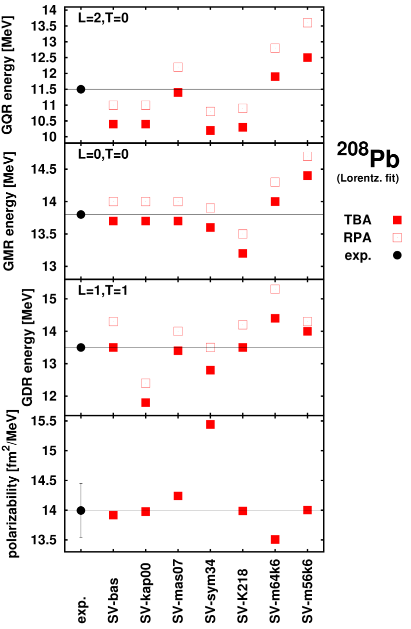
Figure 8: Comparison of giant resonance energies in ²⁰⁸Pb for a variety of Skyrme parameter sets as indicated. The energy centroids $E_{0}=m_{1}/m_{0}$ are computed in the window $E_{0}\pm 2\delta$ where $\delta$ is a dispersion (with the condition $\delta\geq 2$MeV).Open and filled symbols show the values calculated in the framework of RPA and TBA, respectively. The experimental data are taken from Refs. Belyaev et al. (1995) for the GDR, Youngblood et al. (2004) for the GMR and the GQR, and Tamii et al. (2011) for $\alpha_{D}$.

Fig. 8 summarizes the centroids for the three major giant resonances in ²⁰⁸Pb (upper and middle) and the dipole polarizability $\alpha_{D}$ (lower panel). Let us briefly recall the trends for RPA. Changing $\kappa_{\mathrm{TRK}}$ affects almost exclusively the GDR such that lower $\kappa_{\mathrm{TRK}}$ yields a lower peak position. Changing $m^{*}/m$ affects the GQR where lower $m^{*}/m$ means higher peak position. Changing $a_{\mathrm{sym}}$ affects the dipole polarizability $\alpha_{D}$ with larger $a_{\mathrm{sym}}$ enhancing $\alpha_{D}$ although we see also a small side effect on $\alpha_{D}$ from changing $m^{*}/m$. Changing $K$ has an impact predominantly on the GMR where lower $K$ lowers the peak energy. The combined changes of NMP in the two parametrizations SV-m64k6 and SV-m56k6 yield changes in every mode.

The effect of the phonon coupling (move from open to closed symbols) does not change these trends in general. The effects in details depend very much on the actual parametrization but in all cases the energies are shifted downwards. The lower panel of Fig. 8 shows the dipole polarizability $\alpha_{D}$. At first glance, one misses the open symbols. The point is that the polarizability represents a static response and TBA by virtue of the subtraction method is designed such that it leaves stationary states unchanged. Thus RPA and TBA results for $\alpha_{D}$ are exactly the same which simplifies discussions in this case. The large deviation of $\alpha_{D}$ for SV-sym34 is the obvious effect of $a_{\mathrm{sym}}$. It is noteworthy that the combination of changes on NMP in SV-m56k6 cooperates to a good description of $\alpha_{D}$. Here, the low $a_{\mathrm{sym}}$ alone would have produced a to low $\alpha_{D}$. But the low $m^{*}/m$ drives $\alpha_{D}$ back up again.

Figure 9: As figure 8, but for ¹⁶O.

Fig. 9 shows the same for the light nucleus ¹⁶O. As it is well known the standard Skyrme forces produce all too low GDR energies (second panel from below) while those with exotically low effective mass (SV-m56k6 and SV-m64k6) perform fine. The situation is exactly opposite for the GQR (upper panel). Here the standard forces do well and the exotic ones fail. The GMR is badly reproduced. All forces yield a too high centroid energy. As the GMR and GQR are nearly continuously distributed the definition of a centroid energy and a width is probably meaningless as it does not at all characterize the experimental situation. To summarize the situation one may conclude: For ²⁰⁸Pb alone, the conventional RPA using the SV-bas parametrization manages to provide a good description for all four features. However, SV-bas fails badly for the GDR in ¹⁶O and to some extend also for the polarizability (the mismatch of GMR is ignored here). It is only the new force SV-m56k6 in combination with TBA which manages to get the GDR correct in both nuclei Lyutorovich et al. (2012). But this spoils GMR, GQR, and $\alpha_{D}(^{16}\mathrm{O})$. Considering the whole synopsis, we realize that there is no force which reproduces all three giant resonances and the polarizability simultaneously in ¹⁶O and ²⁰⁸Pb, neither for RPA nor for TBA. Harmonizing all results remains a challenge for future research. The situation in ⁴⁰Ca and ⁴⁸Ca resembles more ²⁰⁸Pb as we have already seen in the previous section. Therefore we may characterize the resonances by centroid energy and a width.

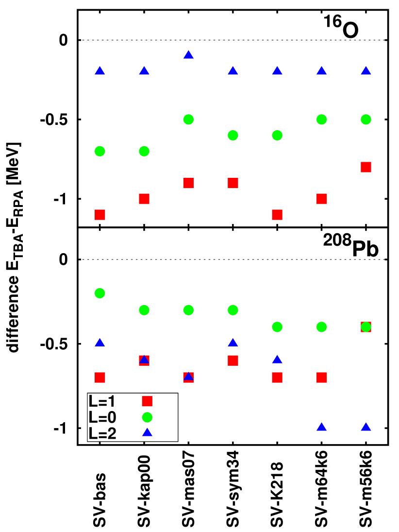
Figure 10: Difference between TBA and RPA for the giant resonance energies in ²⁰⁸Pb and ¹⁶O for a variety of Skyrme parametrizations as indicated.

Fig. 10 shows the differences of the energy centroids between TBA and RPA for ²⁰⁸Pb and ¹⁶O. In this figure the effects are much better presented than in the previous ones where we showed the absolute values. in all cases the TBA energies are lower than the RPA results. This is probably due to the first order correction in the energy dependence of the effective mass discussed in section II.A. The shifts are between one MeV for the GDR in ¹⁶O and about 200 keV for the GQR in the same nucleus. The energy shift of individual modes are always of the same magnitude.

IV.2 Final results compared with experiments

The RPA and TBA theories work best in heavy nuclei where we have a large s.p. basis which gives rise to very many low-lying and high-lying collective phonons. This is the reason why in ²⁰⁸Pb for all Skyrme parametrization we used, theory and experiment for all three giant resonance modes are nearly in quantitative agreement as far as the height of the cross sections and the widths are concerned. We recognize a strong reduction and the corresponding broadening of the RPA cross sections due to the phonon coupling. The mean energies of the resonances on the other hand depend to some extend on the specific Skyrme parametrization used. This is also true for ⁴⁰Ca and ⁴⁸Ca whereas in ¹⁶O only the GDR is well reproduced but not the two isoscalar modes as we have already seen in the previous chapter.

If we compare the shell structure of light nuclei such as ¹⁶O with that of heavy mass nuclei such as ²⁰⁸Pb then one recognizes that light nuclei posses only a very limited number of occupied states which can support $1p1h$ excitations and thus a low density of $1p1h$ states. In ²⁰⁸Pb, on the other hand, one has 126 occupied neutron states and 82 proton states which all give rise to $1p1h$ excitations. This leads to a high density of $1p1h$ states and subsequently rather smooth strength distributions already at the level of RPA. Moreover, light nuclei such as ¹²C and ¹⁶O contain a non-negligible amount of more complicated sub-structures as, e. g., $\alpha$-clusters. This is probably the reason, as already discussed above and in Chapter III, that we can not reproduce the isoscalar modes.

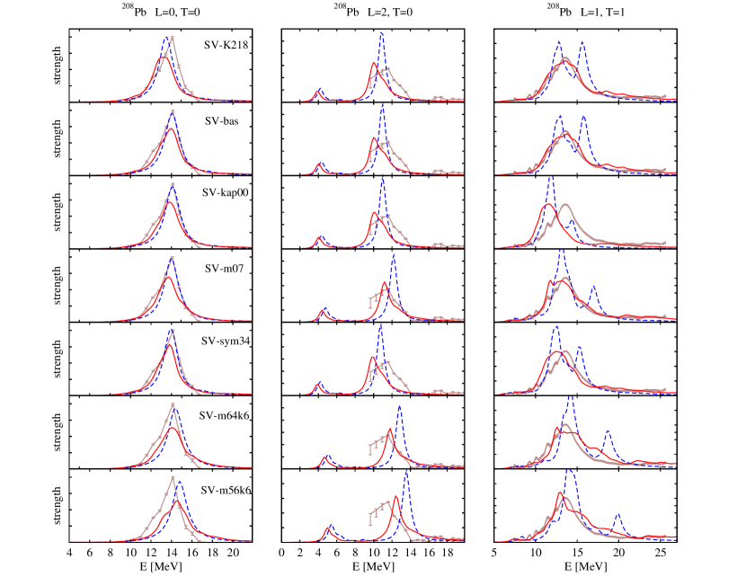
Figure 11: Detailed spectral strength distributions for ²⁰⁸Pb and the the three modes under consideration: isoscalar monopole (left panels), isoscalar quadrupole (middle panels), and isovector dipole (right panels). Photo-absorption strength is shown in case of the dipole mode. Results are obtained with the seven Skyrme parametrizations which we discussed in Chapter IIB. Compared are strengths derived from RPA (blue dashed) and TBA (full red) with experimental data (full brown) from Belyaev et al. (1995) for the GDR and Youngblood et al. (2004) for the GMR and the GQR.

In Fig. 11, the theoretical cross section of GMR, GQR and GDR are compared with the experimental ones for ²⁰⁸Pb. The theoretical results are calculated with all seven Skyrme parameter sets which we presented in Table 1 of Sec. II.B. We first discuss the GMR which is closely connected with the incompressibility $K$. The first four parameter sets have an incompressibility of 234 MeV. The shape of the theoretical cross sections and mean energies of all four parameter sets agree well with the data except the peak height of the theoretical cross section is slightly too low. As three of the parameter set have the same effective mass of $m^{*}/m=0.9$, it is not surprising that the theoretical results are the same. But also the fourth set (SV-mas07) which has an effective mass of $m^{*}/m=0.7$ yields essentially the same cross section. The largest difference delivers set SV-m56k6 with an effective mass of $m^{*}/m=0.56$. Here the theoretical peak in the cross section is about 1.5 MeV to high.

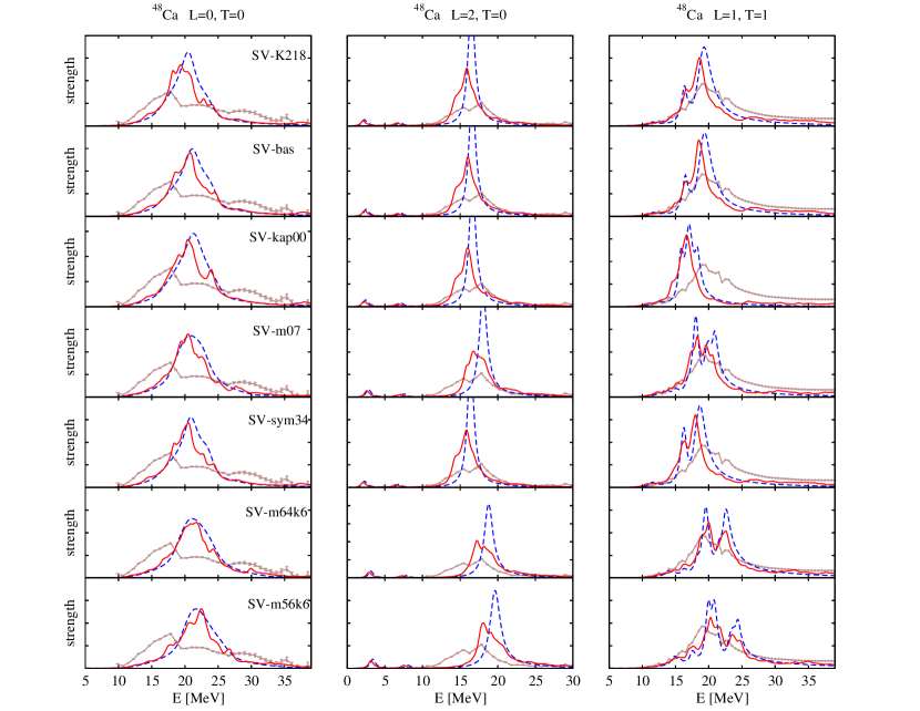
Figure 12: Same results as in the previous figure but for ⁴⁸Ca. The data are taken from Erokhova et al. (2003) for the GDR and from Anders et al. (2013) for the GMR and the GQR.

In Fig. 12 we compare our theoretical results for ⁴⁸Ca with the data. The GDR with the specifically adjusted parameter sets Lyutorovich et al. (2012) to reproduce the GDR in ²⁰⁸Pb and ¹⁶O shown in the last two rows agree nicely with the data. For the other parameter sets the agreement is also not bad. The height of the theoretical cross section for all isoscalar resonances are roughly a factor two too large compared with the experimental ones. Here we have to bear in mind that also deep-lying hole states are important which are very broad. Their widths are insufficiently described by RPA phonons alone and therefore the theoretical resonances are too narrow.

V Summary

The present paper is an extended version of a previous short note Lyutorovich et al. (2015). It is concerned with the time-blocking approximation (TBA) which is an extension of the widely used random-phase approximation (RPA) by complex configurations in terms of $1p1h$ states coupled to RPA phonons and addresses a couple of basic questions in this scheme: proper treatment of the continuum, restoration of stability of ground and excited states, and size of phonon space.

First, we explain here details of the self-consistent continuum TBA which is a new method for handling the single-particle continuum. This method had been further developed to include also the spin-orbit contribution such that our new calculations are fully self-consistent. We then present numerical results which demonstrate the advantages of the continuum treatment as compared to the conventional treatment in a discrete basis.

The phonon coupling modifies the residual two-body interaction which, in principle, would require to compute a new, correlated ground state in order to stay consistent and to achieve a stable excitation spectrum with non-imaginary excitation energies. However, this would introduce a double counting because most ground-state correlations are already incorporated in an effective mean-field theory. The problem is solved by the subtraction scheme, subtracting the stationary (zero-frequency) part of the effective interaction. This leaves the ground state unchanged and delivers stable excitations throughout. It also helps to achieve convergence with phonon number.

A long standing problem concerns the stability of the TBA with respect to the choice of the number of phonons and the size of the single particle space. Here we present the results of detailed calculations with systematically scanned numbers of phonons. An important result is that the energies and widths are stable over a large range if the subtraction method is included in the TBA. This identifies a window of phonon numbers where the results are robust.

Having a well tested numerical scheme for (continuum) RPA and TBA at hand, we investigate the dependence of the three main giant resonances on the basic properties of a Skyrme parameterization: incompressibility, iso-scalar effective mass, symmetry energy and TRK sum rule enhancement. And we do that for RPA in comparison to TBA. TBA generally down-shifts the peak resonance energies by up to 1 MeV. The shift is about same for all parameterizations for a given mode and nucleus. It differs for the three modes and also depends on the nucleus. Although the results show a reasonable general agreement with the data, a parameterization which is able to describe equally well all three resonance modes in heavy as well as light nuclei has not been found.

Appendix A Continuum in a discrete basis representation

In the RPA and TBA the response function $R(\omega)$ is a solution of the Bethe-Salpeter equations (9) and (17), respectively. The propagator $R^{(0)}_{\vphantom{1}}(\omega)$ in these equations in the discrete basis representation has the form

$$R^{(0)}_{ph,p^{\prime}h^{\prime}}(\omega)=-\frac{\delta^{\vphantom{*}}_{pp^{\prime}}\delta^{\vphantom{*}}_{h^{\prime}h}}{\omega-\varepsilon^{\vphantom{*}}_{ph}}\,,$$ (26)

$$R^{(0)}_{hp,h^{\prime}p^{\prime}}(\omega)=\frac{\delta^{\vphantom{*}}_{p^{\prime}p}\delta^{\vphantom{*}}_{hh^{\prime}}}{\omega+\varepsilon^{\vphantom{*}}_{ph}}\,,$$ (27)

where $\varepsilon^{\vphantom{*}}_{ph}=\varepsilon^{\vphantom{*}}_{p}-\varepsilon^{\vphantom{*}}_{h}$.

Let us represent Eqs. (26) and (27) in the form

$$R^{(0)}_{ph,p^{\prime}h^{\prime}}(\omega)=-\delta^{\vphantom{*}}_{h^{\prime}h}\,\langle\,p\,|\,G^{\mbox{\scriptsize MF}(+)}(\varepsilon^{\vphantom{*}}_{h}+\omega)\,|\,p^{\prime}\rangle,$$ (28)

$$R^{(0)}_{hp,h^{\prime}p^{\prime}}(\omega)=-\delta^{\vphantom{*}}_{hh^{\prime}}\,\langle\,p^{\prime}|\,G^{\mbox{\scriptsize MF}(+)}(\varepsilon^{\vphantom{*}}_{h}-\omega)\,|\,p\,\rangle,$$ (29)

where

$$G^{\mbox{\scriptsize MF}(+)}(\varepsilon)=G^{\mbox{\scriptsize MF}}(\varepsilon)-\sum_{h}\frac{|\,h\,\rangle\langle\,h\,|}{\varepsilon-\varepsilon^{\vphantom{*}}_{h}}\,,$$ (30)

$G^{\mbox{\scriptsize MF}}(\varepsilon)$ is the single-particle mean-field Green function, $|\,p\,\rangle$ and $|\,h\,\rangle$ are the single-particle wave functions of particles and holes. The superscript $(+)$ in the notation $G^{\mbox{\scriptsize MF}(+)}(\varepsilon)$ means that this function has the poles only above Fermi level. The equivalence of Eqs. (26)–(27) and (28)–(29) follows from the spectral expansion

$$G^{\mbox{\scriptsize MF}}(\varepsilon)=\sum_{h}\frac{|\,h\,\rangle\langle\,h\,|}{\varepsilon-\varepsilon^{\vphantom{*}}_{h}}+\sum_{p}\frac{|\,p\,\rangle\langle\,p\,|}{\varepsilon-\varepsilon^{\vphantom{*}}_{p}}$$ (31)

and the orthonormality of the wave functions of the discrete basis.

The discrete basis in this scheme is defined as a complete set of solutions of the Schrödinger equation with the box boundary conditions (b.b.c.). Let us introduce another complete set of solutions of this equation obtained by imposing continuum wave boundary conditions (c.b.c.). This set includes a finite number of the discrete states of holes and particles and a particle continuum. Respective mean-field Green functions and the single-particle states will be denoted as $\tilde{G}^{\mbox{\scriptsize MF}}(\varepsilon)$, $|\,\tilde{p}\,\rangle$ and $|\,\tilde{h}\,\rangle$.

The method of inclusion of the continuum in the discrete basis representation consists in the replacement of the uncorrelated $ph$ propagator $R^{(0)}_{\vphantom{1}}(\omega)$ in Eqs. (9) and (17) by the propagator $\tilde{R}^{(0)}_{\vphantom{1}}(\omega)$, which is defined by the formulas:

$$\tilde{R}^{(0)}_{ph,p^{\prime}h^{\prime}}(\omega)=-\delta^{\vphantom{*}}_{h^{\prime}h}\,\langle\,p\,|\,\tilde{G}^{\mbox{\scriptsize MF}(+)}(\varepsilon^{\vphantom{*}}_{h}+\omega)\,|\,p^{\prime}\rangle,$$ (32)

$$\tilde{R}^{(0)}_{hp,h^{\prime}p^{\prime}}(\omega)=-\delta^{\vphantom{*}}_{hh^{\prime}}\,\langle\,p^{\prime}|\,\tilde{G}^{\mbox{\scriptsize MF}(+)}(\varepsilon^{\vphantom{*}}_{h}-\omega)\,|\,p\,\rangle,$$ (33)

$$\tilde{G}^{\mbox{\scriptsize MF}(+)}(\varepsilon)=\tilde{G}^{\mbox{\scriptsize MF}}(\varepsilon)-\sum_{\tilde{h}}\frac{|\,\tilde{h}\,\rangle\langle\,\tilde{h}\,|}{\varepsilon-\varepsilon^{\vphantom{*}}_{\tilde{h}}}\,.$$ (34)

Eqs. (32)–(33) are obtained from Eqs. (28)–(29) by the replacement of the function $G^{\mbox{\scriptsize MF}(+)}(\varepsilon)$ by the function $\tilde{G}^{\mbox{\scriptsize MF}(+)}(\varepsilon)$. The Green function $\tilde{G}^{\mbox{\scriptsize MF}}(\varepsilon)$ in Eq. (34) is calculated via the regular and irregular solutions of the Schrödinger equation (with c.b.c.) by means of the known technique Shlomo and Bertsch (1975). The matrix elements of $\tilde{G}^{\mbox{\scriptsize MF}(+)}(\varepsilon)$ are calculated with particle wave functions $|\,p\,\rangle$ and $|\,p^{\prime}\rangle$ of the discrete basis. Thus, the RPA and the TBA equations (9) and (17) are solved in the discrete basis representation. However, in contrast to the initial uncorrelated $ph$ propagator $R^{(0)}_{\vphantom{1}}(\omega)$, the propagator $\tilde{R}^{(0)}_{\vphantom{1}}(\omega)$ does not contain the discrete poles $\omega=\pm\varepsilon^{\vphantom{*}}_{ph}$ corresponding to the transitions between the hole states and the discrete particle states with positive energies, since these states are replaced by the continuum included in the Green function $\tilde{G}^{\mbox{\scriptsize MF}}(\varepsilon)$.

This method recovers the exact method Shlomo and Bertsch (1975) of treatment of the continuum in the coordinate representation if the discrete basis is sufficiently complete and the radius of the box is sufficiently large to ensure the equality $|\,h\,\rangle=|\,\tilde{h}\,\rangle$.

As a criterion of the fulfillment of this equality we choose the absolute value of the difference between the energies of the hole states calculated with continuum wave boundary and box boundary conditions, respectively: $\Delta\varepsilon^{\vphantom{*}}_{h}=\varepsilon^{\vphantom{*}}_{h}-\varepsilon_{\tilde{h}}$. In all our calculations (with $R_{\mbox{\scriptsize box}}=15$ fm for ¹⁶O, ⁴⁰Ca, and ⁴⁸Ca and $R_{\mbox{\scriptsize box}}=18$ fm for ¹³²Sn and ²⁰⁸Pb) we have $\max|\Delta\varepsilon^{\vphantom{*}}_{h}|\lesssim 10^{-5}$ MeV.

References

- Vretenar et al. (2005) D. Vretenar, A. V. Afanasjev, G. Lalazissis, and P. Ring, Phys. Rep. 409, 101 (2005).
- Bender et al. (2003) M. Bender, P.-H. Heenen, and P.-G. Reinhard, Rev. Mod. Phys. 75, 121 (2003).
- Goriely et al. (2002) S. Goriely, M. Samyn, P. H. Heenen, J. M. Pearson, and F. Tondeur, Phys. Rev. C 66, 024326 (2002).
- Kortelainen et al. (2010a) M. Kortelainen, T. Lesinski, J. Moré, W. Nazarewicz, J. Sarich, N. Schunck, M. V. Stoitsov, and S. Wild, Phys. Rev. C 82, 024313 (2010a).
- Maruhn et al. (2014) J. A. Maruhn, P.-G. Reinhard, P. D. Stevenson, and A. S. Umar, Comp. Phys. Comm. 185, 2195 (2014).
- Drożdż et al. (1990) S. Drożdż, S. Nishizaki, J. Speth, and J. Wambach, Phys. Rep. 197, 1 (1990).
- Dehesa et al. (1977) J. Dehesa, S. Krewald, J. Speth, and A. Faessler, Phys. Rev. C 15, 1858 (1977).
- Tselyaev (1989) V. I. Tselyaev, Yad. Fiz.; Soviet Journal of Nuclear Physics (English translation) 50, 1252 (1989).
- Tselyaev (2007) V. I. Tselyaev, Phys. Rev. C 75, 024306 (2007), arXiv:nucl-th/0505031 [nucl-th] .
- Lyutorovich et al. (2015) N. Lyutorovich, V. Tselyaev, J. Speth, S. Krewald, F. Grümmer, and P.-G. Reinhard, Phys. Lett. B 749, 292 (2015).
- Kamerdzhiev et al. (1993) S. Kamerdzhiev, J. Speth, G. Tertychny, and V. Tselyaev, Nucl. Phys. A 555, 90 (1993).
- Kamerdzhiev et al. (2004) S. Kamerdzhiev, J. Speth, and G. Tertychny, Phys. Rep. 393, 1 (2004), arXiv:nucl-th/0311058 [nucl-th] .
- Litvinova and Tselyaev (2007) E. V. Litvinova and V. I. Tselyaev, Phys. Rev. C 75, 054318 (2007).
- Berman and Fultz (1975) B. L. Berman and S. C. Fultz, Rev. Mod. Phys. 47, 713 (1975).
- Klüpfel et al. (2009) P. Klüpfel, P. G. Reinhard, T. J. Bürvenich, and J. A. Maruhn, Phys. Rev. C 79, 034310 (2009).
- Erler et al. (2011) J. Erler, P. Klüpfel, and P. G. Reinhard, J. Phys. G 38, 033101 (2011).
- Erler et al. (2010) J. Erler, P. Klüpfel, and P. . G. Reinhard, J. Phys. G 37, 064001 (2010), http://www.arxiv.org/abs/1002.0027.
- Abrahamyan et al. (2012) S. Abrahamyan, Z. Ahmed, H. Albataineh, K. Aniol, D. S. Armstrong, W. Armstrong, T. Averett, B. Babineau, A. Barbieri, V. Bellini, R. Beminiwattha, J. Benesch, F. Benmokhtar, T. Bielarski, W. Boeglin, A. Camsonne, M. Canan, P. Carter, G. D. Cates, C. Chen, J. P. Chen, O. Hen, F. Cusanno, M. M. Dalton, R. De Leo, K. de Jager, W. Deconinck, P. Decowski, X. Deng, A. Deur, D. Dutta, A. Etile, D. Flay, G. B. Franklin, M. Friend, S. Frullani, E. Fuchey, F. Garibaldi, E. Gasser, R. Gilman, A. Giusa, A. Glamazdin, J. Gomez, J. Grames, C. Gu, O. Hansen, J. Hansknecht, D. W. Higinbotham, R. S. Holmes, T. Holmstrom, C. J. Horowitz, J. Hoskins, J. Huang, C. E. Hyde, F. Itard, C. M. Jen, E. Jensen, G. Jin, S. Johnston, A. Kelleher, K. Kliakhandler, P. M. King, S. Kowalski, K. S. Kumar, J. Leacock, J. Leckey, J. H. Lee, J. J. LeRose, R. Lindgren, N. Liyanage, N. Lubinsky, J. Mammei, F. Mammoliti, D. J. Margaziotis, P. Markowitz, A. McCreary, D. McNulty, L. Mercado, Z. E. Meziani, R. W. Michaels, M. Mihovilovic, N. Muangma, C. Muñoz-Camacho, S. Nanda, V. Nelyubin, N. Nuruzzaman, Y. Oh, A. Palmer, D. Parno, K. D. Paschke, S. K. Phillips, B. Poelker, R. Pomatsalyuk, M. Posik, A. J. R. Puckett, B. Quinn, A. Rakhman, P. E. Reimer, S. Riordan, P. Rogan, G. Ron, G. Russo, K. Saenboonruang, A. Saha, B. Sawatzky, A. Shahinyan, R. Silwal, S. Sirca, K. Slifer, P. Solvignon, P. A. Souder, M. L. Sperduto, R. Subedi, R. Suleiman, V. Sulkosky, C. M. Sutera, W. A. Tobias, W. Troth, G. M. Urciuoli, B. Waidyawansa, D. Wang, J. Wexler, R. Wilson, B. Wojtsekhowski, X. Yan, H. Yao, Y. Ye, Z. Ye, V. Yim, L. Zana, X. Zhan, J. Zhang, Y. Zhang, X. Zheng, and P. Zhu (PREX Collaboration), Phys. Rev. Lett. 108, 112502 (2012).
- Tamii et al. (2011) A. Tamii, I. Poltoratska, P. von Neumann-Cosel, Y. Fujita, T. Adachi, C. A. Bertulani, J. Carter, M. Dozono, H. Fujita, K. Fujita, K. Hatanaka, D. Ishikawa, M. Itoh, T. Kawabata, Y. Kalmykov, A. M. Krumbholz, E. Litvinova, H. Matsubara, K. Nakanishi, R. Neveling, H. Okamura, H. J. Ong, B. Özel-Tashenov, V. Y. Ponomarev, A. Richter, B. Rubio, H. Sakaguchi, Y. Sakemi, Y. Sasamoto, Y. Shimbara, Y. Shimizu, F. D. Smit, T. Suzuki, Y. Tameshige, J. Wambach, R. Yamada, M. Yosoi, and J. Zenihiro, Phys. Rev. Lett. 107, 062502 (2011).
- Savran et al. (2011) D. Savran, M. Elvers, J. Endres, M. Fritzsche, B. Löher, N. Pietralla, V. Y. Ponomarev, C. Romig, L. Schnorrenberger, K. Sonnabend, and A. Zilges, Phys. Rev. C 84, 024326 (2011).
- Horowitz and Piekarewicz (2001) C. J. Horowitz and J. Piekarewicz, Phys. Rev. Lett. 86, 5647 (2001).
- Lyutorovich et al. (2012) N. Lyutorovich, V. I. Tselyaev, J. Speth, S. Krewald, F. Grümmer, and P. G. Reinhard, Phys. Rev. Lett. 109, 092502 (2012).
- Lyutorovich et al. (2016) N. Lyutorovich, V. Tselyaev, J. Speth, S. F. Krewald, and P.-G. Reinhard, to be published in Phys. At. Phys., (2016), arXiv:1602.00862.
- Brown (1971) G. E. Brown, Unified Theory of Nuclear Models and Forces, 3rd ed. (North-Holland, Amsterdam, London, 1971).
- Speth et al. (1977) J. Speth, E. Werner, and W. Wild, Phys. Rep. 33, 127 (1977).
- Jeukenne et al. (1976) J. P. Jeukenne, A. Lejeune, and C. Mahaux, Phys. Rep. 25, 83 (1976).
- Grümmer and Speth (2006) F. Grümmer and J. Speth, J. Phys. G: Nucl. Part. Phys. 32, R193 (2006).
- Wambach et al. (1982) J. Wambach, V. Mishra, and L. Chu-Hsia, Nucl. Phys. A380, 285 (1982).
- Kamerdzhiev et al. (1997) S. P. Kamerdzhiev, G. Y. Tertychny, and V. I. Tselyaev, Fiz. Elem. Chastits At. Yadra; Phys. Part. Nucl. 28, 333, 134 (1997).
- Toepffer and Reinhard (1988) C. Toepffer and P.-G. Reinhard, Ann. Phys. (N.Y.) 181, 1 (1988).
- Tselyaev (2013) V. I. Tselyaev, Phys. Rev. C 88, 054301 (2013).
- Stone and Reinhard (2007) J. R. Stone and P. . G. Reinhard, Prog. Part. Nucl. Phys. 58, 587 (2007), http://www.arxiv.org/abs/nucl-th/0607002.
- Kortelainen et al. (2010b) M. Kortelainen, T. Lesinski, J. Moré, W. Nazarewicz, J. Sarich, et al., Phys. Rev. C 82, 024313 (2010b), arXiv:1005.5145 [nucl-th] .
- Myers (1977) W. D. Myers, Droplet Model of Atomic Nuclei (IFI/Plenum, New York, 1977).
- Nazarewicz et al. (2014) W. Nazarewicz, P. G. Reinhard, W. Satula, and D. Vretenar, Eur. Phys. J. A 50, 20 (2014), arXiv:1307.5782.
- Shlomo and Bertsch (1975) S. Shlomo and G. Bertsch, Nucl. Phys. A 243, 507 (1975).
- Tondeur et al. (1984) F. Tondeur, M. Brack, M. Farine, and J. M. Pearson, Nucl. Phys. A 420, 297 (1984).
- Tselyaev et al. (2009) V. Tselyaev, J. Speth, S. Krewald, E. Litvinova, S. Kamerdzhiev, N. Lyutorovich, A. Avdeenkov, and F. Grümmer, Phys. Rev. C 79, 034309 (2009).
- Bohigas et al. (1979) O. Bohigas, A. Lane, and J. Martorell, Phys. Rep. 51, 267 (1979).
- Klüpfel et al. (2008) P. Klüpfel, J. Erler, P. . G. Reinhard, and J. A. Maruhn, Eur. Phys. J. A 37, 343 (2008), http://www.arxiv.org/abs/0804.340.
- Nakatsukasa and Yabana (2005) T. Nakatsukasa and K. Yabana, Phys. Rev. C 71, 024301 (2005).
- De Donno et al. (2011) V. De Donno, G. Co’, M. Anguiano, and A. M. Lallena, Phys. Rev. C 83, 044324 (2011).
- Lui et al. (2001) Y.-W. Lui, H. L. Clark, and D. H. Youngblood, Phys. Rev. C 64, 064308 (2001).
- Ishkhanov et al. (2002) B. S. Ishkhanov, I. M. Kapitonov, E. I. Lileeva, E. V. Shirokov, V. A. Erokhova, M. A. Yolkin, and A. V. Izotova, Preprint INP MSU 2002-27/711 (2002).
- Anders et al. (2013) M. R. Anders, S. Shlomo, T. Sil, D. H. Youngblood, Y.-W. Lui, and Krishichayan, Phys. Rev. C 87, 024303 (2013).
- Erokhova et al. (2003) V. A. Erokhova, M. A. Elkin, A. V. Izotova, B. S. Ishkhanov, L. M. Kapitonov, E. I. Lileeva, and E. V. Shirokov, Izv. Ross. Akad. Nauk. Ser. Fiz.. 67, 1479 (2003).
- Knöpfle et al. (1978) K. Knöpfle, G. Wagner, C. Mayer-Böricke, M. Rogge, and P. Turek, Phys. Lett. B 74, 191 (1978).
- Belyaev et al. (1995) S. N. Belyaev, O. V. Vasiliev, V. V. Voronov, A. A. Nechkin, V. Y. Ponomarev, and V. A. Semenov, Phys. Atom. Nucl. 58, 1883 (1995).
- Youngblood et al. (2004) D. H. Youngblood, Y.-W. Lui, H. L. Clark, B. John, Y. Tokimoto, and X. Chen, Phys. Rev. C 69, 034315 (2004).