Exact solution of equations for proton localization in neutron star matter

Abstract

The rigorous treatment of proton localization phenomenon in asymmetric nuclear matter is presented. The solution of proton wave function and neutron background distribution is found by the use of the extended Thomas-Fermi approach. The minimum of energy is obtained in the Wigner-Seitz approximation of spherically symmetric cell. The analysis of three different nuclear models suggests that the proton localization is likely to take place in the interior of neutron star.
PACS number(s): 21.65.Cd, 21.65.Mn, 26.60.-c

I Introduction

The interior of a neutron star contains the densest forms of matter in the Universe. The central density is as high as 5 to 10 times the nuclear equilibrium density $n_{0}=0.16~{}\rm fm^{-3}$. Most of the mass of the star is placed in its liquid core covered by a thin crust ($<1\rm~{}km$ for typical neutron star) whose bottom edge is located at around 0.5$n_{0}$. Above this density the matter is well described by the Fermi liquid - a mixture of nucleons and leptons. In comparison to the matter present inside the stable nuclei, the matter in neutron star is highly asymmetric as a consequence of the $\beta$-equilibrium taking place between nucleons and leptons. It is convenient to express the asymmetry by the proton fraction $x=n_{p}/n$, where $n_{p},n$ are the proton and baryon number density. The proton fraction is between 0.4 and 0.5 in nuclei, whereas in neutron star matter at $n_{0}$ it is equal to 4% what is exactly determined by the saturation point properties. The proton abundance at higher density is not well known and different nuclear interactions models lead to a very large discrepancies in the $x(n)$ behaviour. There are models which predict that $x$ does not exceed 10% in a full range of densities. When the proton fraction is not high, protons can be treated as the small admixture to the neutron background, where direct proton-proton interaction is negligible and hence protons can be regarded as impurities in the neutron matter. Therefore, a description of this system by single proton in neutron background is justified. The attractive nature of proton-neutron interaction may result in an instability of homogeneously distributed protons kutschera89 ; kutschera90 ; kutschera93 . In the paper kutschera93 the polaron behaviour of a proton impurity in dense neutron matter was discussed. A single proton in neutron matter can lower its energy by inducing the density inhomogeneity around it. Instead of forming the Fermi sea, protons occupy ground state with zero momentum above some critical density. It occurs when the localized proton with properly distorted neutron background has smaller energy than the system with the proton described by the plane waves. Such a state of matter has intriguing magnetic properties that has been shown in kutschera89 ; kutschera94 ; kutschera97 . It exhibits, e.g. a crystallization of proton impurities in the neutron star interior kutschera95 ; potekhin10 and affects the cooling process of neutron stars baiko99 ; baiko00 . In the papers kutschera90 ; kutschera93 the proton localization has been analyzed in a simplified manner. A variational approach to a cell containing one proton was proposed. However, the minimization of the energy was achieved with respect to Gaussian-type trial function with only one parameter for both proton wave function and neutron background. Moreover, the cell was treated as a system with infinite volume $V\rightarrow\infty$ which means that the method is applicable to a very small ($x$ smaller than 1%) proton fraction.

The aim of this work is to solve exactly the Lagrange-Euler equations corresponding to the variational approach proposed in the original works. We also abandon the assumption of infinitely large cell. This means we may take into account higher proton fractions and thus, extent the class of nuclear models in the analysis.

The equation of state of supra-nuclear density in a neutron star core cannot be calculated unambiguously lattimer07 ; haensel06 . Instead, there are many theoretical models of exotic matter. We choose two representatives of them satisfying the criterion of maximum mass greater then $2M_{\odot}$ maxmass1 ; maxmass2 and leading, at the same time, to not very high proton fraction at higher densities: AV14+UVII wff88 , SLy4 chabanat98 . The last one is very common in the description of the neutron stars as it well reproduces the properties of nuclei, the nucleon-nucleon scattering data, and it correctly recovers saturation point properties. Moreover, in our analysis we also included UV14+TNI model taken from lagaris81 . Although the maximum neutron star mass for this model is smaller than $2M_{\odot}$, it was interesting to test it for very small proton fractions at high density because it could be relevant for the properties of proton localization. In the Fig.1 the proton fraction in $\beta$-equilibrated matter is shown for the three selected nuclear models.

The present paper is organized as follows. A short review of the the variational method for finite-size Wigner-Seitz cell is presented in Sec.II. In Sec.III the numerical method for solving the equations is explained. The results are shown and discussed for various nuclear models in Sec.IV.

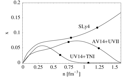
Figure 1: The proton fraction for different models used in the calculation: AV14+UVII, SLy4 and UV14+TNI. The squares indicate the proton localization threshold and the full dots indicate the central density of a star with maximum mass.

II A proton in neutron background

In order to calculate the energy of nuclear matter with localized protons we treat the proton as a quantum particle described by its wave function $\Psi(\mbox{\boldmath$r$})$ whereas the neutrons are represented by a density distribution function $n_{n}(\mbox{\boldmath$r$})$. Like in the work kutschera93 we assume that one proton occupies a spherical Wigner-Seitz (W-S) cell filled with large number of neutrons. Neutrons are treated in the local density approximation according to differential Thomas-Fermi scheme bbp71 . The energy of the cell is expressed by the integral over the whole cell volume $V_{WS}=1/\bar{n}_{p}$

$$E[\psi,n_{n}] ={\displaystyle\int_{V_{WS}}} \left[\Psi^{*}(-\frac{\nabla^{2}}{2m_{p}}+\mu_{p})\Psi\right.$$ (1)

$$\Big{.}+\;\varepsilon+B_{N}(\nabla n_{n})^{2}\Big{]}d^{3}r.$$

The nuclear matter energy density $\varepsilon$ is the thermodynamical function which depends directly on nucleon densities $\varepsilon(n_{n},n_{p})$. Its functional form is completely determined by the adopted nuclear model. The chemical potentials are defined as usual

$$\mu_{p}=\left(\frac{\partial\varepsilon}{\partial n_{p}}\right)\raisebox{-10.00002pt}{$n_{n}$}~{}~{},~{}~{}\mu_{n}=\left(\frac{\partial\varepsilon}{\partial n_{n}}\right)\raisebox{-10.00002pt}{$n_{p}$}.$$ (2)

In the energy functional Eq. (1) the energy density $\varepsilon$ and the proton chemical potential $\mu_{p}$ get the space dependence by the local neutron density: $\varepsilon(r)=\varepsilon(n_{n}(r),0)$ and in the same way $\mu_{p}(r)=\mu_{p}(n_{n}(r),0)$. The constant coefficient $B_{N}$ describes the gradient contribution and it is fitted to the surface properties of nuclei, here we adopt the value $B_{N}=31.6~{}\rm MeV\;fm^{5}$ kutschera90 .

The W-S cell radius is given by the proton density for homogeneous system $R_{WS}=(3/4\pi\bar{n}_{p})^{1/3}$, where $\bar{n}_{p}=xn$ and $n$ is the mean baryon number.

The cell energy should be minimized under constraints of fixed proton and neutron number

$${\displaystyle\int_{V_{WS}}} \Psi^{*}\Psi d^{3}r=1,$$ (3)

$${\displaystyle\int_{V_{WS}}} n_{n}d^{3}r=V_{WS}\bar{n}_{n},$$ (4)

where $\bar{n}_{n}=(1-x)n$ is the mean neutron number in the case of homogeneous system. The constraints expressed by Eqs. (3,4) require the following Lagrange multipliers $\lambda_{p},\lambda_{n}$:

$$\tilde{E}=E-\lambda_{p}\int(\Psi^{*}\Psi-1/V_{WS})d^{3}r-\lambda_{n}\int(n_{n}-\bar{n}_{n})d^{3}r.$$ (5)

For the isolated, spherically symmetric W-S cell we impose the following boundary conditions:

$$\frac{\partial\Psi}{\partial r}(0)=0 ~{}~{},~{}~{} \Psi(R_{WS})=0~{},$$

$$\frac{\partial n_{n}}{\partial r}(0)=0 ~{}~{},~{}~{} \frac{\partial n_{n}}{\partial r}(R_{WS})=0~{}.$$ (6)

From the Lagrange-Euler equations for the minimum of $\tilde{E}$ one may remark that the Lagrange multipliers $\lambda_{p}$ and $\lambda_{n}$ correspond to the physical quantities such as the eigenvalue $E_{p}$ of the proton wave function and the neutron chemical potential $\mu_{n}$ at the cell boundary:

$$\lambda_{p}=E_{p}~{}~{},~{}~{}\lambda_{n}=\mu_{n}|_{R_{WS}},$$ (7)

and then, finally, one may write the Lagrange-Euler equations in the form

$$\frac{-\nabla^{2}}{2m_{p}}\Psi+\mu_{p}\Psi=E_{p}\Psi,$$ (8)

$$\frac{\partial\mu_{p}}{\partial n_{n}}\Psi^{*}\Psi+\Delta\mu_{n}-2B_{N}\nabla^{2}n_{n}=0,$$ (9)

where $\Delta\mu_{n}=\mu_{n}(n_{n}(r),0)-\mu_{n}|_{R_{WS}}$ is the difference between local chemical potential and its boundary value. The first equation Eq. (8) represents the Schrödinger equation for the spherically symmetric proton wave function $\Psi(r)$ with the eigenvalue $E_{p}$. The coupling to neutron density $n_{n}(r)$ comes from the chemical potential $\mu_{p}(n_{n},0)$. The second equation Eq. (9) is the nonlinear elliptic equation for the neutron density distribution $n_{n}(r)$ coupled to the proton density $\Psi^{*}\Psi$.

The proton localization occurs if at a given mean density $n$ there exists a proton wave function with a negative eigenvalue $E_{p}<0$ and when the energy of homogeneous system of nucleons is greater than the energy $E[\Psi,n_{n}]$ of system with distorted densities, that means

$$\Delta E=E[\Psi,n_{n}]-\varepsilon(n(1\!-\!x),nx)V_{WS}<0.$$ (10)

In this way, by solving the Eqs. (8,9), we obtain a family of solutions parametrized with the mean density of matter $n$.

III The method

The mean baryon density $n$ does not enter directly to the Eqs. (8,9). The average density $n$ is determined indirectly by the second constraint, Eq.(4). Therefore, in numerical solving it is simpler to set the value at the boundary

$$n_{n}^{\infty}\equiv n_{n}|_{R_{WS}}~{},$$ (11)

find the proton function and neutron background and then finally derive the mean density from the relation

$$n=\frac{1}{V_{WS}}\left(1+\int_{V_{WS}}n_{n}(r)d^{3}r\right)~{}.$$ (12)

The set of Eqs.(8,9) was solved by the relaxation method explained in the following.

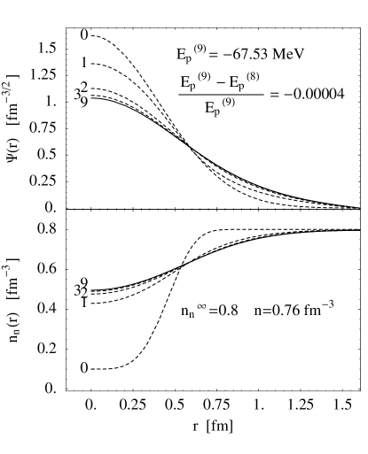
Figure 2: The subsequent steps in the relaxation method for proton wave function $\psi(r)$ (upper panel) and neutron density $n_{n}(r)$ (lower panel) in the nuclear model AV14+UVII. The solid curve represents the final results after 9 steps when the accuracy equal to $10^{-4}$ was achieved for ground energy $E_{p}$.

As an initial approximation, the Gaussian-type function was taken for the proton wave function and for the neutron density. In the $i$-th step, the iteration had two stages: in the first we found the ground state solution $\Psi^{(i+1)}~{},E_{p}^{(i+1)}$ of Schrödinger equation including $n_{n}^{(i)}$. In the second step we solve the Eq. (9) for $n_{n}^{(i+1)}$ including $\Psi^{(i+1)}$. The iteration was continued up to the point where the eigenvalue does not change more than a given accuracy. The procedure appeared to converge quickly, usually the accuracy equal to $10^{-4}$ was achieved in not more than 15 steps. The Fig.2 represents the convergence of the iteration for the chosen density $n_{n}^{\infty}=0.8$ in the AV14+UVII model.

IV Results

The proton localization scheme described in the previous sections was then analyzed for the three nuclear models: AV14+UVII, SLy4 and UV14+TNI. For all of them the proton localization turned out to occur. Comparing the localization threshold obtained here with the results of previous works based on approximate variational method with Gaussian proton profile (see Table I in szmaglinski06 ) one observe systematically lower values resulting from the present method. For example: AV14+UVII - 0.789 (old) and 0.745 (new), UV14+TNI - 0.731 and (old) 0.608 (new) in $\rm fm^{-3}$. As a conclusion one may say that the correction to the threshold density is of the order of 10%. It seems natural that new values of $n_{loc}$ are a little smaller since in our calculations both proton wave function and neutron background present exact solutions of assumed equations.

Table 1: Various parameters above the threshold on the proton localization.

	$n_{n}^{\infty}\rm~{}[fm^{-3}]$	$n~{}[\rm fm^{-3}]$	$\Delta E/A\rm~{}[MeV]$	$E_{p}$  [MeV]	$\langle r_{p}\rangle[\rm fm]$
SLy4	0.785	0.805	0	-45.99	0.674
	0.879	0.905	-1.55	-84.63	0.606
	0.972	1.007	-3.73	-131.18	0.548
	1.066	1.110	-6.75	-185.01	0.500
	1.160	1.214	-10.81	-245.55	0.459
AV14+UVII	0.745	0.763	0	-33.97	0.747
	0.861	0.885	-3.52	-114.48	0.624
	0.978	1.005	-8.41	-230.13	0.528
	1.094	1.123	-13.44	-376.14	0.456
	1.210	1.239	-16.98	-550.70	0.404
UV14+TNI	0.610	0.608	0	-23.62	1.023
	0.725	0.723	-0.22	-71.83	0.826
	0.840	0.838	-0.50	-137.2	0.660
	0.955	0.954	-0.80	-213.0	0.564
	1.070	1.069	-1.08	-297.0	0.500

The two models (SLy4, AV14+UVII) were analyzed in the whole range of available density: from the threshold for localization (see first row for a particular model in the Table 1) to the maximum density which is determined by the maximum neutron star mass (the squares and full dots in the Fig. 1). In the case of the third one (UV14+TNI), the range of density relevant for localization was between the threshold and the point where the protons disappear that means $x=0$. It occurs for $n=1.07~{}\rm fm^{-3}$. In the Fig.3 and Fig.4 the evolution with the baryon density of proton wave function and neutron background distribution is shown. The vertical lines indicate the W-S cell radius $R_{WS}$. For the SLy4 model the $R_{WS}$ takes the smallest values which means that the cell contains about ten neutrons. For the rest of the models, the $R_{WS}$ is greater and W-S cell containers from 10 to several hundred of neutrons which justifies the description of neutrons by its local density $n_{n}(r)$.

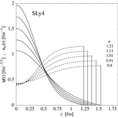
Figure 3: The evolution of proton wave function (solid) and neutron background (dashed) with increasing mean baryon density $n$ for the SLy4 nuclear model. Vertical lines indicate the position of $R_{WS}$.

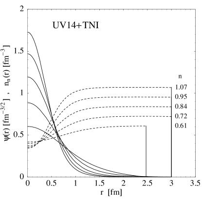
Figure 4: The same like in the Fig.3 for the UV14+TNI nuclear model. For densities above $0.7~{}\rm fm^{-3}$ the $R_{WS}$ was greater than $3~{}\rm fm^{-3}$.

The behaviour of the proton wave function and neutron density is similar as in the previous approximate calculations kutschera90 ; kutschera93 ; kutschera02 . The proton mean radius $\langle r_{p}\rangle$ decreases whereas the depth of the neutron well increases with the mean density of matter. The particular values of quantities relevant for the proton localization are shown in the Table 1. First two columns present the neutron density $n_{n}^{\infty}$ at the W-S boundary Eq. (11) and the mean baryon density $n$. The $\Delta E/A$ is the energy difference between the homogeneous matter and the state with localized proton Eq. (10) taken per total number of baryon in the cell. The $E_{p}$ presents the proton energy eigenvalue. For all models the localization energy $\Delta E/A$ increases with the density and the same happens to the proton energy $E_{p}$, so one may conclude the proton is localized stronger at higher densities. An interesting fact is that, in case of UV14+TNI model, although the proton fraction is very small, the strength of localization, measured by the energy difference $\Delta E/A$ takes the smallest values in comparison to the other models.

V Summary

In the present work we have solved the Lagrange-Euler equations for a proton impurity with the extended Thomas-Fermi approach for neutron background. The proton was treated as quantum particle immersed in the quasi-classical neutron sea. In a previous work the proton abundance was assumed to be infinitely small, e.i. the Wigner-Seitz cell was infinitely large, $R_{WS}\rightarrow\infty$. Here we kept finite $R_{WS}$ determined by the proton fraction which is fixed by the $\beta$-equilibrium occurring in neutron star matter. By minimization of the energy in the finite-size Wigner-Seitz cell we found exact solution for proton wave function and neutron background. It turn out that proton localization still occurs for all the presented models. The localization threshold is slightly lower than in the previous work where the one-parameter method for energy minimization was used kutschera02 . In this work we have investigated, in a rigorous way, the earlier ideas of the proton localization and have shown the phenomenon is plausible and worth further research. Interesting issues involve: the crystallization of protons as has been shown earlier kutschera95 , the influence of temperature on the neutron threshold density for proton localization skw14 and consequences for neutron star cooling baiko99 ; baiko00 .

References

- (1) M. Kutschera and W. Wójcik, Phys. Lett. B 223, 11 (1989).
- (2) M. Kutschera and W. Wójcik, Acta Phys. Polon. B 21, 823 (1990).
- (3) M. Kutschera, W. Wójcik, Phys. Rev. C 47, 1077 (1993).
- (4) M. Kutschera, S. Stachniewicz, A. Szmagliński, and W. Wójcik, Acta Phys. Polon. B 33, 743 (2002).
- (5) A. Szmagliński, W. Wójcik and M. Kutschera, Acta Phys. Polon. B 37, 277 (2006).
- (6) M. Kutschera and W. Wójcik, Acta Phys. Polon. B 23, 947 (1992).
- (7) M. Kutschera and W. Wójcik, Phys. Lett. B 325, 271 (1994).
- (8) M. Kutschera and W. Wójcik, Acta Phys. Polon. A, 92, 375 (1997).
- (9) M. Kutschera and W. Wójcik, Nucl. Phys. A 581, 706 (1995).
- (10) A. Y. Potekhin, Usp. Fiz. Nauk 180, 1279 (2010).
- (11) D. A. Baiko and P. Haensel, Acta Phys. Polon. B 30, 1097 (1999).
- (12) D. A. Baiko and P. Haensel, Astron. Astrophys. 356, 171 (2000).
- (13) J. M. Lattimer and M. Prakash, Phys. Rep. 550, 109 (2007).
- (14) P. Haensel, A. Y. Potekhin, and D. G. Yakovlev, in Neutron Stars 1: Equation of State and Structure (Springer, Berlin, 2006).
- (15) P. B. Demorest, T. Pennucci, S. M. Ransom, M. S. E. Roberts, and J. W. T. Hessels, Nature 467, 1081 (2010).
- (16) J. Antoniadis et.al, Science 340, 6131 (2013).
- (17) R. B. Wiringa, V. Fiks, and A. Fabrocini, Phys. Rev. C 38, 1010 (1988).
- (18) E. Chabanat, P. Bonche, P. Haensel, J. Meyer, and R. Schaeffer, Nucl. Phys. A 635, 231 (1998).
- (19) I. E. Lagaris and V. R. Pandharipande, Nucl. Phys. A 359, 349 (1981).
- (20) G. Baym, H. A. Bethe, and C. Pethick, Nucl. Phys. A 175, 225 (1971).
- (21) A. Szmagliński, S. Kubis, and W. Wójcik, Acta Phys. Polon. B 45, 249 (2014).