Effective potential from zero-momentum potential

Abstract:

We obtain the centre-of-mass frame effective potential from the zero-momentum potential in Ruijsenaars-Schneider type 1-dimensional relativistic mechanics using classical inverse scattering methods.

1 Introduction and motivation

Recent advances in lattice QCD make it possible to measure relevant physical quantities at realistic, physical quark masses. This includes the measurement of the nuclear force between nucleons by the HAL QCD collaboration [1, 2, 3]. The HAL QCD method is based on the Nambu-Bethe-Salpeter (NBS) wave function defined by

$$\psi^{\rm NBS}_{\bf k}({\bf x})=\langle 0|N({\bf 0},0)N({\bf x},0)|{\rm NN};{\bf k}\rangle^{\rm in},$$ (1)

where $\langle 0|$ is the QCD vacuum state, $|{\rm NN};{\bf k}\rangle^{\rm in}$ is a 2-nucleon scattering state in the centre-of-mass (COM) frame with nucleon momenta ${\bf k}$ and $-{\bf k}$ and total COM energy $W=2\sqrt{{\bf k}^{2}+m^{2}}$, $m$ is the nucleon mass and $N({\bf x},t)$ is a local nucleon field operator. Both the nucleon field operators and the 2-nucleon state depend on additional quantum numbers (total spin $S$, isospin, etc.), which are suppressed in the above formula for simplicity.

The reason to call the object defined by this formula a wave function is that it can be shown that at large nucleon separation ($r=|{\bf x}|\to\infty$) the interaction between them can be neglected and it behaves like a free wave function:

$$(k^{2}+{\bf\nabla}^{2})\psi^{\rm NBS}_{\bf k}({\bf x})\approx 0,\qquad\quad k=|{\bf k}|.$$ (2)

Moreover, it can also be shown [3, 4] that its radial component behaves for large separation $r$ as

$$\phi^{\rm NBS}_{k}(r;L,S)\approx\frac{\sin(kr-L\pi/2+\delta_{LS}(k))}{kr}{\rm e}^{i\delta_{LS}(k)},$$ (3)

where $L$ is the total angular momentum of the 2-nucleon state. Thus the exact scattering phase shifts $\delta_{LS}(k)$ are encoded in the NBS wave function. But it contains much more information and motivated by the above wave function interpretation one can define the NBS potential by writing

$$(E_{\bf k}-H_{o})\psi^{\rm NBS}_{\bf k}({\bf x})=U^{\rm NBS}_{\bf k}({\bf x})\psi^{\rm NBS}_{\bf k},$$ (4)

where

$$E_{\bf k}=\frac{{\bf k}^{2}}{2M},\qquad H_{o}=-\frac{1}{2M}{\bf\nabla}^{2}$$ (5)

and $M$ is the reduced mass $M=m/2$. This resembles the non-relativistic Schrödinger equation with potential $U^{\rm NBS}_{\bf k}({\bf x})$. Indeed, the lattice measurements found that $U^{\rm NBS}_{\bf k}({\bf x})$ is very similar to the phenomenological nuclear potential. At large distance it has an attractive tail, but at shorter distances it develops a characteristic repulsive core (RC). While the long distance attraction has long been understood by nuclear theorists and it is due to meson exchanges, it was the first time that the RC has been obtained from a first principles calculation.

Later the same method has been successfully applied also to other hadronic interactions: this included the baryon-baryon potential [5, 6] and the study of 3-body nuclear forces [7]. Short distance behaviour of the NBS wave function and potential can be analytically studied, thanks to the asymptotic freedom property of QCD, by operator product expansion and renormalization group techniques [8, 9, 10, 11, 12].

Despite these successes, there are also some serious open problems within this approach. First, the wave function depends on the choice of the interpolating field $N({\bf x},t)$ used for nucleons. While in lattice studies $N({\bf x},t)$ was naturally represented by a local, gauge invariant 3-quark operator, it is not known to what extent the resulting NBS potential depends on this choice. Secondly, unlike the potential term in the Schrödinger equation, $U^{\rm NBS}_{\bf k}({\bf x})$ is energy (momentum) dependent due to the relativistic nature of the problem. A possible solution of this problem is to define [2, 3] a new, non-local, but energy independent potential operator. This non-local operator can be approximated by a series containing terms with derivative operators of increasing power. The leading term is a local potential and it is again similar to the phenomenological potential. Alternatively, since the energy dependence is weak at low energies, one can define the zero-momentum potential

$$U_{o}({\bf x})=\lim_{{\bf k}\to 0}U^{\rm NBS}_{\bf k}({\bf x}).$$ (6)

It can be shown [13] that $U_{o}$ correctly reproduces the scattering lengths, but already the next to leading order parameter for low energy scattering, the effective range, may differ from the true one.

The problem of energy dependence has been studied in some $1+1$ dimensional integrable field theory models [13], where the NBS wave function can be represented by the form factor expansion. In these studies the Ising model and the O$(3)$ nonlinear sigma model were considered and it was found that $U_{o}({\bf x})$ is indeed a good approximation at low energies where the energy dependence is weak.

A more interesting toy model to study would be the sine-Gordon (SG) model, because unlike in the Ising model and the O$(3)$ model (which are free and repulsive, respectively), here we have both repulsive (soliton-soliton) and attractive (soliton-antisoliton) scattering and in addition there are soliton-antisoliton bound states (breathers). The form factors are in principle available also for this model, but to construct the NBS wave function via the form factor expansion would be very involved technically. Luckily, an alternative description of the SG model exists since it is known that for any fixed particle number subspace of the SG field theory Hilbert space there is a corresponding Ruijsenaars-Schneider (RS) type relativistic quantum mechanical description [14]. The RS wave function is known [15] for both soliton-soliton and soliton-antisoliton scattering and exactly reproduces the scattering phase shifts of SG field theory. Moreover, also the soliton-antisoliton bound state spectrum is calculable and exactly match the SG results.

In this paper we take one more backward step and consider the classical relativistic RS 2-particle scattering problem. Energy dependence of the potential is already present in this system but here the problem can be completely solved using textbook results for classical inverse scattering. We can find the relation between the zero-momentum potential and the true effective potential analytically. One can hope that the zero-momentum potential versus effective potential relation can similarly be found in the relativistic RS quantum mechanical problem, using the existing methods of quantum inverse scattering.

The paper is organized as follows. In section 2 we review the RS type relativistic 2-particle mechanics. In section 3 we construct the effective potential using classical inverse scattering, which is described in detail (adapted to and generalized for our problem) in the appendix of the paper. We give our conclusions in section 4.

2 Ruijsenaars-Schneider type 2-particle problem

Ruijsenaars-Schneider type models are a particular realization of the Hamiltonian construction of relativistic point particle interaction in $1+1$ dimension. The starting point for the latter is the relativistic phase space spanned by the canonical variables $q_{a}$, $\theta_{b}$ satisfying

$$\{q_{a},q_{b}\}=\{\theta_{a},\theta_{b}\}=0,\qquad\quad\{q_{a},\theta_{b}\}=\delta_{ab},\qquad a,b=1,2\dots,N.$$ (7)

For relativistic invariance we have to construct the three generators of the $1+1$ dimensional Poincaré group, the Hamiltonian ${\cal H}$, the momentum ${\cal P}$, and the Lorentz-boost ${\cal K}$, which satisfy the Poisson-bracket relations

$$\{{\cal H},{\cal P}\}=0,\qquad\quad\{{\cal H},{\cal K}\}={\cal P},\qquad\quad\{{\cal P},{\cal K}\}=\frac{1}{c^{2}}{\cal H}.$$ (8)

Using the Hamiltonian vector fields $\hat{\cal H}$ and $\hat{\cal P}$ associated with ${\cal H}$ and ${\cal P}$ respectively, we can calculate the time and space derivatives of any phase space function ${\cal F}$ by the usual formulas

$$\hat{\cal H}{\cal F}=\{{\cal H},{\cal F}\}=\dot{\cal F},\qquad\quad\hat{\cal P}{\cal F}=\{{\cal P},{\cal F}\}={\cal F}^{\prime}.$$ (9)

Further we can calculate the time and space “flows” of the canonical coordinates by solving the differential equations

$$\frac{\partial}{\partial t}Q_{a}(t;q,\theta)=\dot{q}_{a}(Q,T),\qquad\frac{\partial}{\partial t}T_{b}(t;q,\theta)=\dot{\theta}_{b}(Q,T)$$ (10)

with initial conditions

$$Q_{a}(0;q,\theta)=q_{a},\qquad\quad T_{b}(0;q,\theta)=\theta_{b}$$ (11)

for the time flow $Q_{a}(t;q,\theta)$, $T_{b}(t;q,\theta)$ and

$$\frac{\partial}{\partial x}\bar{Q}_{a}(x;q,\theta)=q_{a}^{\prime}(Q,T),\qquad\frac{\partial}{\partial x}\bar{T}_{b}(x;q,\theta)=\theta^{\prime}_{b}(Q,T)$$ (12)

with initial conditions

$$\bar{Q}_{a}(0;q,\theta)=q_{a},\qquad\quad\bar{T}_{b}(0;q,\theta)=\theta_{b}$$ (13)

for the space flow $\bar{Q}_{a}(t;q,\theta)$, $\bar{T}_{b}(t;q,\theta)$.

The final step is finding the physical particle coordinates $x_{a}(q,\theta)$, $a=1,2,\dots,N$ as functions of the phase space variables. The construction we are using here is explained in [16] and is based on $N$ Lorentz-invariant (not Poincaré invariant!) phase space functions $\rho_{a}(q,\theta)$,

$$\hat{\cal K}\rho_{a}=\{{\cal K},\rho_{a}\}=0,\qquad\quad a=1,2,\dots,N.$$ (14)

Given $\rho_{a}$, we can calculate its space flow

$$R_{a}(x;q,\theta)=\rho_{a}(\bar{Q},\bar{T})$$ (15)

and the trajectory variable (coordinate) of the $a^{\rm th}$ particle is defined by the implicit equation

$$R_{a}(x_{a};q,\theta)=0.$$ (16)

Finally the time-dependent trajectory is given by

$$x_{a}(t;q,\theta)=x_{a}(Q,T).$$ (17)

The Ruijsenaars-Schneider Ansatz [14] for two particles is of the form

$${\cal H}=mc^{2}(\cosh\theta_{1}+\cosh\theta_{2})f(q_{1}-q_{2}),\qquad{\cal P}=mc(\sinh\theta_{1}+\sinh\theta_{2})f(q_{1}-q_{2}),$$ (18)

$${\cal K}=-\frac{1}{c}(q_{1}+q_{2}),$$ (19)

where $m$ is the mass of the particles and $f(q)$ is an even, positive real function, which we can parametrize as

$$f^{2}(q)=1+b(q).$$ (20)

$b(q)$ is, as we will see, the zero-momentum potential (up to rescaling). It is easy to check that the relations (8) are satisfied for any such $f(q)$.

The best known examples are of hyperbolic type,

$$b(q)=\frac{\gamma^{2}}{\sinh^{2}(\omega q)}\qquad{\rm and}\qquad b(q)=-\frac{\gamma^{2}}{\cosh^{2}(\omega q)}.$$ (21)

The inverse $\sinh^{2}$ potential is monotonically repulsive (MR, see A.2) whereas the negative inverse $\cosh^{2}$ potential is of LA type (see A.4). The constant $\omega$ can be written as $1/mc\ell$ where $\ell$ is a length scale, and the dimensionless coupling constant $\gamma$ is restricted in the LA case by $\gamma\leq 1$. The Sine-Gordon model corresponds to the choice $\gamma=1$ [14].

For the construction of the trajectory variables we can use [14]

$$\rho_{a}(q,\theta)=q_{a},\qquad\quad R_{a}(x;q,\theta)=\bar{Q}_{a}(x;q,\theta).$$ (22)

It turns out to be useful to introduce the centre-of-mass and relative coordinates and momenta

$$\zeta=q_{1}+q_{2},\qquad q=q_{1}-q_{2};\qquad\quad 2\tau=\theta_{1}+\theta_{2},\qquad 2u=\theta_{1}-\theta_{2}.$$ (23)

In terms of these,

$${\cal H}=2mc^{2}\varepsilon\cosh\tau,\qquad\quad{\cal P}=2mc\varepsilon\sinh\tau,$$ (24)

which shows that

$$\varepsilon=f(q)\cosh u$$ (25)

is the (Poincaré invariant) total mass, normalized to $1$, and the meaning of $\tau$ is the rapidity of the COM of the 2-particle system.

It is easy to see that

$$\dot{\tau}=0\qquad\quad{\rm and}\qquad\quad\dot{\zeta}=-2mc\varepsilon\sinh\tau,$$ (26)

thus it is consistent to go to the COM system $\tau=\zeta=0$. This simplifies the construction of the trajectory variables enormously and we find that in the COM system

$$x_{1}=-x_{2}=\frac{q}{2mc\varepsilon}.$$ (27)

For the remaining relative variables $q$, $u$ we introduce the corresponding time flows $Q$, $U$. We also introduce the relative physical coordinate

$$y(t)=x_{1}(t)-x_{2}(t)=\frac{Q}{mc\varepsilon}.$$ (28)

The COM dynamics of the 2-particle Ruijenaars-Schneider model is equivalent to the conservation law

$$\frac{1}{4}\dot{y}^{2}+\frac{1}{\varepsilon^{2}}W_{o}(\varepsilon y)=H^{\rm NR}={\rm const.},$$ (29)

where

$$W_{o}(x)=c^{2}b(mcx)$$ (30)

is the zero-momentum potential. The energy constant is given by

$$H^{\rm NR}=c^{2}\left(1-\frac{1}{\varepsilon^{2}}\right).$$ (31)

For scattering states of asymptotic velocity $v$ (in the COM system), where

$$\varepsilon=\frac{1}{\sqrt{1-\frac{v^{2}}{c^{2}}}}$$ (32)

we have

$$H^{\rm NR}=v^{2},$$ (33)

whereas for bound states of mass $m_{\rm B}$ (where $\varepsilon=m_{\rm B}/2m$) we can use the parametrization

$$m_{\rm B}=2m-\frac{mh}{c^{2}}\qquad\quad(0\leq h\leq 2c^{2})$$ (34)

and we find

$$H^{\rm NR}=-h\frac{1-\frac{h}{4c^{2}}}{\left(1-\frac{h}{2c^{2}}\right)^{2}}.$$ (35)

(29) looks like a non-relativistic problem, except for rescaling with the state-dependent constant of motion $\varepsilon$. The corresponding NR problem is

$$\frac{1}{4}\dot{z}^{2}+W_{o}(z)=H_{o}={\rm const.},$$ (36)

for the NR variable $z(t)$. (29) and (36) coincide for $v=0$, which justifies the name zero-momentum potential for $W_{o}$.

For the NR problem the energy constant can be written

$$H_{o}=v_{o}^{2}\quad{\rm(scattering)},\qquad\quad H_{o}=-h_{o}\quad{\rm(bound\ state\ problem)},\quad 0\leq h_{o}\leq b_{o}\leq c^{2}.$$ (37)

(Here $-b_{o}$ is the minimum of $W_{o}$.)

The solution of the physical problem (29) is obtained from the solution of the fictious NR problenm (36) by putting

$$y(t)=\frac{1}{\varepsilon}z(t)$$ (38)

and choosing

$$H_{o}=\varepsilon^{2}H^{\rm NR}.$$ (39)

This corresponds to the choice

$$v_{o}=\varepsilon v\quad{\rm(scattering)},\qquad\quad h_{o}=h\left(1-\frac{h}{4c^{2}}\right)\quad{\rm(bound\ state\ problem)}.$$ (40)

3 Effective potential

The following discussion is based on the theory of classical inverse scattering described in appendix A.

Taking into account the $\varepsilon$ dependence of the physical problem and the scaling rules of A.7 we see that the physical (relativistic) scattering data are simply related to the ones calculated in the NR problem:

$$X^{{\rm rel}}(v)=\frac{1}{\varepsilon}X_{o}(\varepsilon v),\qquad\quad P^{{\rm rel}}(h)=P_{o}\left(h\left(1-\frac{h}{4c^{2}}\right)\right).$$ (41)

Here $P$ is the period in case of bound motion and $X(v)=-vT(v)$ is the displacement corresponding to the time delay $T(v)$. The time delay is the classical counterpart of the quantum phase shift. It is the energy derivative of the phase shift in the semiclassical ($\hbar\to 0$) limit. The formula for the displacement becomes especially simple if we introduce the (mass-reduced) momentum variable $q$,

$$p=mq,\qquad\qquad q=\frac{v}{\sqrt{1-\frac{v^{2}}{c^{2}}}}.$$ (42)

We denote the displacement as funtion of this momentum variable by $\tilde{X}^{{\rm rel}}$ and we get

$$\tilde{X}^{{\rm rel}}(q)=\frac{1}{\sqrt{1+\frac{q^{2}}{c^{2}}}}X_{o}(q).$$ (43)

In the bound state problem

$$0\leq h\leq b_{{\rm rel}},$$ (44)

where

$$b_{{\rm rel}}-\frac{b^{2}_{{\rm rel}}}{4c^{2}}=b_{o}\leq c^{2}.$$ (45)

For the Sine-Gordon model soliton-soliton scattering we have to take as zero-momentum potential our $1/\sinh^{2}$ MR example (114) with $g=c$ and we find

$$\tilde{X}^{{\rm rel}}(q)=\frac{\ell}{2}\frac{1}{\sqrt{1+\frac{q^{2}}{c^{2}}}}\ln\left(1+\frac{c^{2}}{q^{2}}\right).$$ (46)

The Sine-Gordon soliton-antisoliton scattering corresponds to the zero-momentum potential $-1/\cosh^{2}$ in our LA example (117) with $g=c$ and as shown in A.9 the scattering displacement formula is exactly the same as (46). For the relativistic period we find

$$P^{{\rm rel}}(h)=\frac{\ell\pi}{\sqrt{h}}\frac{1}{\sqrt{1-\frac{h}{4c^{2}}}},\qquad\quad 0\leq h\leq 2c^{2}.$$ (47)

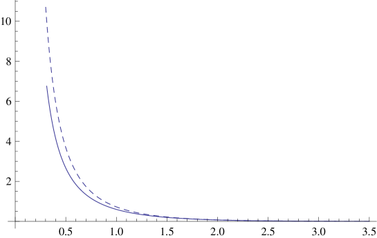
Figure 1: Sine-Gordon effective potential (solid line). The dashed line is the corresponding zero-momentum potential. The plots show $W^{\rm eff}/mc^{2}$ vs. $x/\ell$.

Since the relativistic and NR scattering data are very similar, the following question arises naturally. Is there a NR effective potential $W^{{\rm eff}}$ such that the physical, relativistic scattering data (in the COM frame) are exactly reproduced by using a non-relativistic Hamiltonian with potential $W^{{\rm eff}}$? In other words, we require that

$$\tilde{X}^{{\rm rel}}(q)=X^{{\rm eff}}(q),\qquad\quad P^{{\rm rel}}(h)=P^{{\rm eff}}(h),\quad 0\leq h\leq b_{{\rm rel}},\quad b_{{\rm rel}}=b_{{\rm eff}}.$$ (48)

For the SG soliton-soliton scattering, the answer is yes. We simply take the physical result (46) and use the formulas given in A.8 to obtain the effective potential by using the techniques of classical inverse scattering for MR type potentials. The effective potential is given by an integral formula. The integral cannot be calculated analytically, but it is easily obtained by numerical integration. The result is shown in Fig. 1. From the low energy asymptotics of (46) we can read of the parameters (see A.10)

$${\cal L}=\frac{\ell}{2},\qquad u_{o}=2c,\qquad\hat{\alpha}=\frac{3\ell}{2},\qquad\hat{\beta}=\frac{\ell}{2}$$ (49)

and using the results of A.10 we can determine the large distance asymptotics of the effective potential:

$$U^{{\rm eff}}(x)\approx 4mc^{2}{\rm e}^{-2x/\ell}\left\{1+\left(3-\frac{2x}{\ell}\right){\rm e}^{-2x/\ell}+\dots\right\}$$ (50)

The leading term is the same as for the zero-momentum potential, but the subleading terms differ.

For the Sine-Gordon soliton-antisoliton problem the answer is no. As shown in A.4 for LA type NR potentials there is a constraint between the scattering and bound state data and in this case the constraint (113) between $\tilde{X}^{{\rm rel}}(q)$ and $P^{{\rm rel}}(h)$ is not satisfied. Therefore no $W^{{\rm eff}}(x)$ exists.

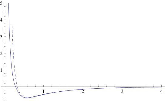
Figure 2: Effective potential for an RC type potential with parameters $\beta=0.3$ and $\xi=1.4$ (solid line). The dashed line is the corresponding zero-momentum potential. The plots show $W^{\rm eff}/mc^{2}$ vs. $x/\ell$.

For our RC example (see A.3, A.9) the answer is again yes. We have to use both $\tilde{X}^{{\rm rel}}(q)$ and $P^{{\rm rel}}(h)$ to determine the two partial inverse functions, which are then used to reconstruct $W^{{\rm eff}}(x)$. We did this numerically. The results are shown in Figs. 2,3, for $\xi=1.4$ and the parameter values $\beta=B/c^{2}=0.3$, $\beta=B/c^{2}=0.7$ respectively.

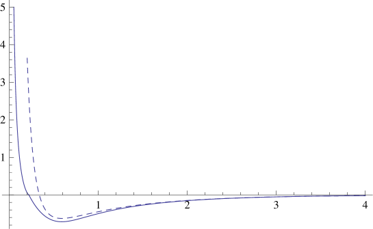
Figure 3: Effective potential for an RC type potential with parameters $\beta=0.7$ and $\xi=1.4$ (solid line). The dashed line is the corresponding zero-momentum potential. The plots show $W^{\rm eff}/mc^{2}$ vs. $x/\ell$.

4 Conclusion

The Nambu-Bethe-Salpeter potential as measured by the HAL QCD collaboration can be identified, at low energies, with the zero-momentum nucleon potential. This can be compared to the phenomenological nuclear potential, which has been constructed to reproduce the nucleon scattering data (at low energies, below the pion production threshold). This problem can be modelled in a $1+1$ dimensional toy model, the Sine-Gordon field theory. For the 2-particle case, one can study the equivalent quantum mechanical problem, the relativistic Ruijsenaars-Schneider model for two particles. In this paper we worked out the zero-momentum potential $\to$ effective potential mapping in the semiclassical limit of the RS model, using classical inverse scattering techniques. It turned out that the very existence of such a mapping depends crucially on the qualitative features of the potential. For repulsive scattering and potentials with a repulsive core, the zero-momentum and effective potentials are qualitatively very similar and quantitatively close at low energies. The first one can be used to describe soliton-soliton scattering in the SG model and the second one is a $1+1$ dimensional model of the nucleon potential. On the other hand, no such mapping exists for soliton-antisoliton scattering and bound states in the SG model.

It is likely that quantum inverse scattering can be applied to study the same questions at the quantum mechanical level in SG/RS theory. Whether the zero-momentum potential $\to$ effective potential mapping exists in the physically relevant $3+1$ dimensional nucleon problem is an open question.

Acknowledgments

This investigation was supported by the Hungarian National Science Fund OTKA (under K83267). J. B. would like to thank the CAS Institute of Modern Physics, Lanzhou, where most of this work has been carried out, for hospitality.

Appendix A Classical inverse scattering

In this appendix we summarize the techniques used for classical inverse scattering.

A.1 Landau-Lifshitz formula

A basic problem in analytic classical mechanics is to reconstruct the potential for a point particle in one dimension if the period of oscillations for the bound motions as function of the energy is known. The solution of this problem can be found in the book of Landau & Lifshitz [17]. We take, for simplicity, a symmetric potential $U(x)$ with $U(0)=0$ which is monotonically increasing for $0\leq x<\infty$ (see Fig. 4). The Landau-Lifshitz trick is to consider instead of the potential its inverse function $\xi(U)$. For a given energy $E$, the bound motion of the particle is confined to $x_{1}\leq x\leq x_{2}$, where $x_{2}=-x_{1}=\xi(E)$.

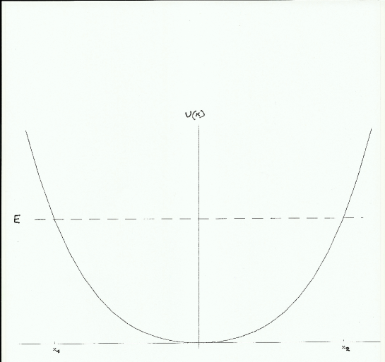
Figure 4: Symmetric potential. The half-period of periodic motion with energy $E$ is the time the particle needs to move between the turning points $x_{1}$ and $x_{2}$.

The half-period of oscillations is easily expressed as

$$T(E)=\sqrt{2m}\int_{0}^{\xi(E)}\frac{{\rm d}x}{\sqrt{E-U(x)}}=\sqrt{2m}\int_{0}^{E}\xi^{\prime}(U)\frac{{\rm d}U}{\sqrt{E-U}}.$$ (51)

The trick is to change the integration variable to $U$. $m$ is the mass of the particle. Given $T(E)$, (51) is an Abel-type linear integral equation for the unknown function $\xi(U)$. The solution is given by the simple formula [17]

$$\xi(U)=\frac{1}{\pi\sqrt{2m}}\int_{0}^{U}\frac{T(E){\rm d}E}{\sqrt{U-E}}.$$ (52)

A.2 Time delay in classical one-dimensional scattering, monotonic repulsive (MR) potential

A similar, but somewhat more complicated problem is to reconstuct the one dimensional potential from the classical time delay in scattering problems. The details of the computation strongly depend on the type of the potential. We start with the simplest case of a monotonically decreasing, repulsive (MR) potential (see Fig. 5). Assuming $U(x)>0$, $U(\infty)=0$ and $U^{\prime}(x)<0$, we can find again the inverse function $\xi(U)$. We will consider a scattering process with fixed energy $E$. The energy can be parametrized as

$$E=\frac{1}{2}mv^{2},$$ (53)

where $v$ is the asymptotic velocity of the particle. The scattering process is infinite so first we calculate the time necessary to reach the point $x_{1}$ starting from the turning point $x_{o}=\xi(E)$:

$$\sqrt{\frac{m}{2}}\int_{x_{o}}^{x_{1}}\frac{{\rm d}x}{\sqrt{E-U(x)}}=-\sqrt{\frac{m}{2}}\int_{U_{1}}^{E}\xi^{\prime}(U)\frac{{\rm d}U}{\sqrt{E-U}}.$$ (54)

If the potential were not there, the particle would move freely with constant velocity $v$ (except from bouncing back from the origin) and the time from $0$ to $x_{1}$ would be

$$\frac{x_{1}}{v}=\sqrt{\frac{m}{2E}}x_{1}.$$ (55)

The time delay $\Delta(E)$ is the time difference between the actual motion and the free one in the limit $x_{1}\to\infty$ ($U_{1}\to 0$):

$$\Delta(E)=-\sqrt{2m}\left\{\frac{\xi(E)}{\sqrt{E}}+\int_{0}^{E}\xi^{\prime}(U){\rm d}U\left[\frac{1}{\sqrt{E-U}}-\frac{1}{\sqrt{E}}\right]\right\}.$$ (56)

The derivation of the above formula is valid if

$$\lim_{x\to\infty}x^{2}U(x)=0,$$ (57)

i.e. if the potential vanishes sufficiently fast at infinity.

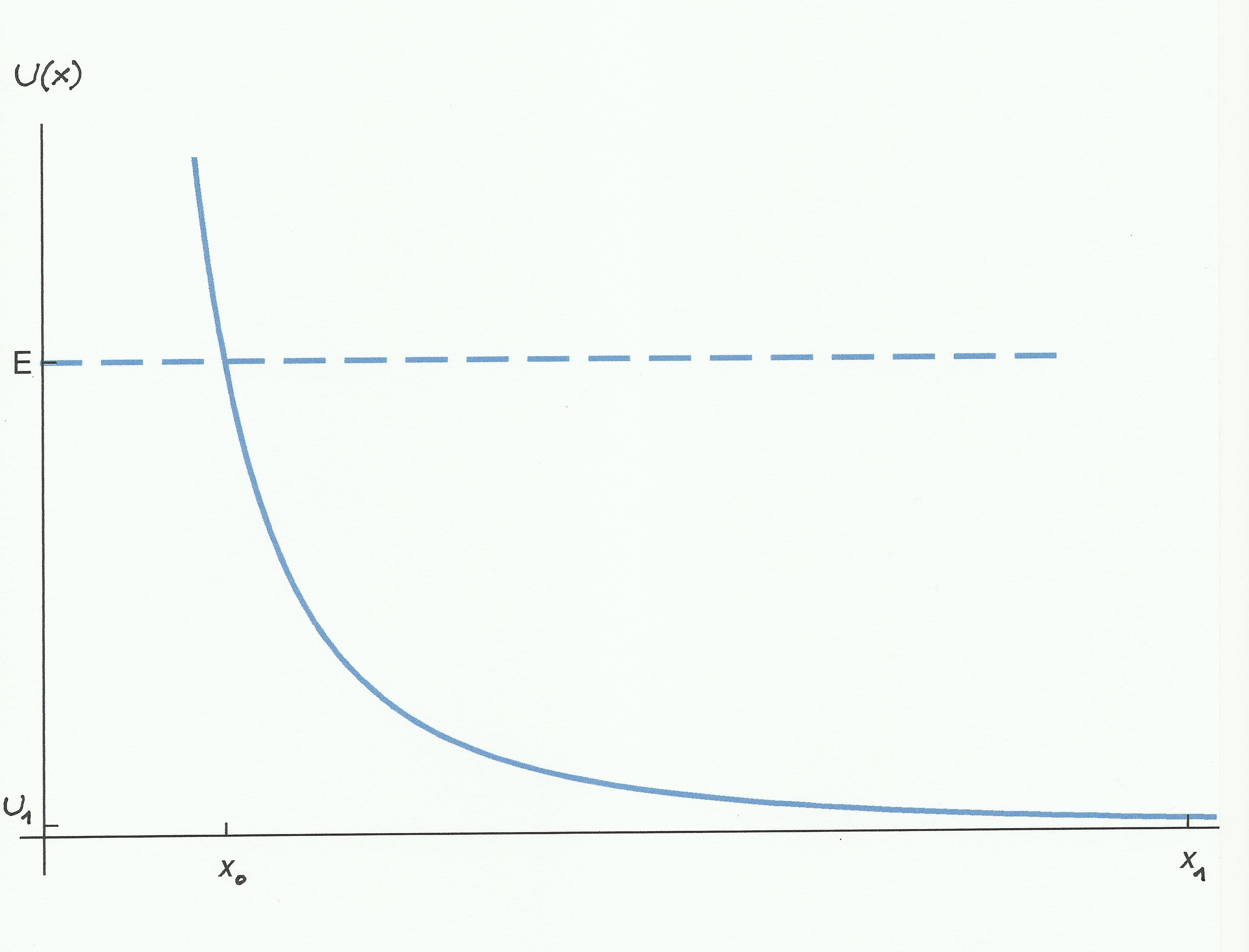
Figure 5: Monotonically repulsive potential. The time delay is the time difference between the actual motion from the turning point $x_{o}$ to $x_{1}$ and the free motion from the origin to a distant point $x_{1}$, in the limit $x_{1}\to\infty$.

Although the formula (56) is more complicated than the one in the previous subsection, the corresponding integral equation can be solved by the same trick with the result

$$\xi(U)=-\frac{1}{\pi\sqrt{2m}}\int_{0}^{U}\frac{\Delta(E){\rm d}E}{\sqrt{U-E}}.$$ (58)

A.3 Potential with repulsive core (RC)

The potential shown in Fig. 6 is a one dimensional model of the nuclear potential. It consists of a monotonically decreasing part ($0<x<x^{*}$) and a monotonically increasing part ($x^{*}<x<\infty$) with $U(\infty)=0$. The minimum of the potential is at $x^{*}$ and it is parametrized as:

$$U(x^{*})=-mb.$$ (59)

Since there is no global inverse function, we have to use the two partial functional inverse functions $\xi_{1}(U)$, $\xi_{2}(U)$. They are defined for $\infty>U\geq-mb$ and $-mb\leq U<0$, respectively and satisfy

$$\xi_{1}(-mb)=\xi_{2}(-mb)=x^{*}.$$ (60)

For motions with negative total energy $-mb<E<0$ it is useful to introduce the “width function”

$$d(V)=\xi_{2}(-V)-\xi_{1}(-V),\qquad\quad 0<V\leq mb.$$ (61)

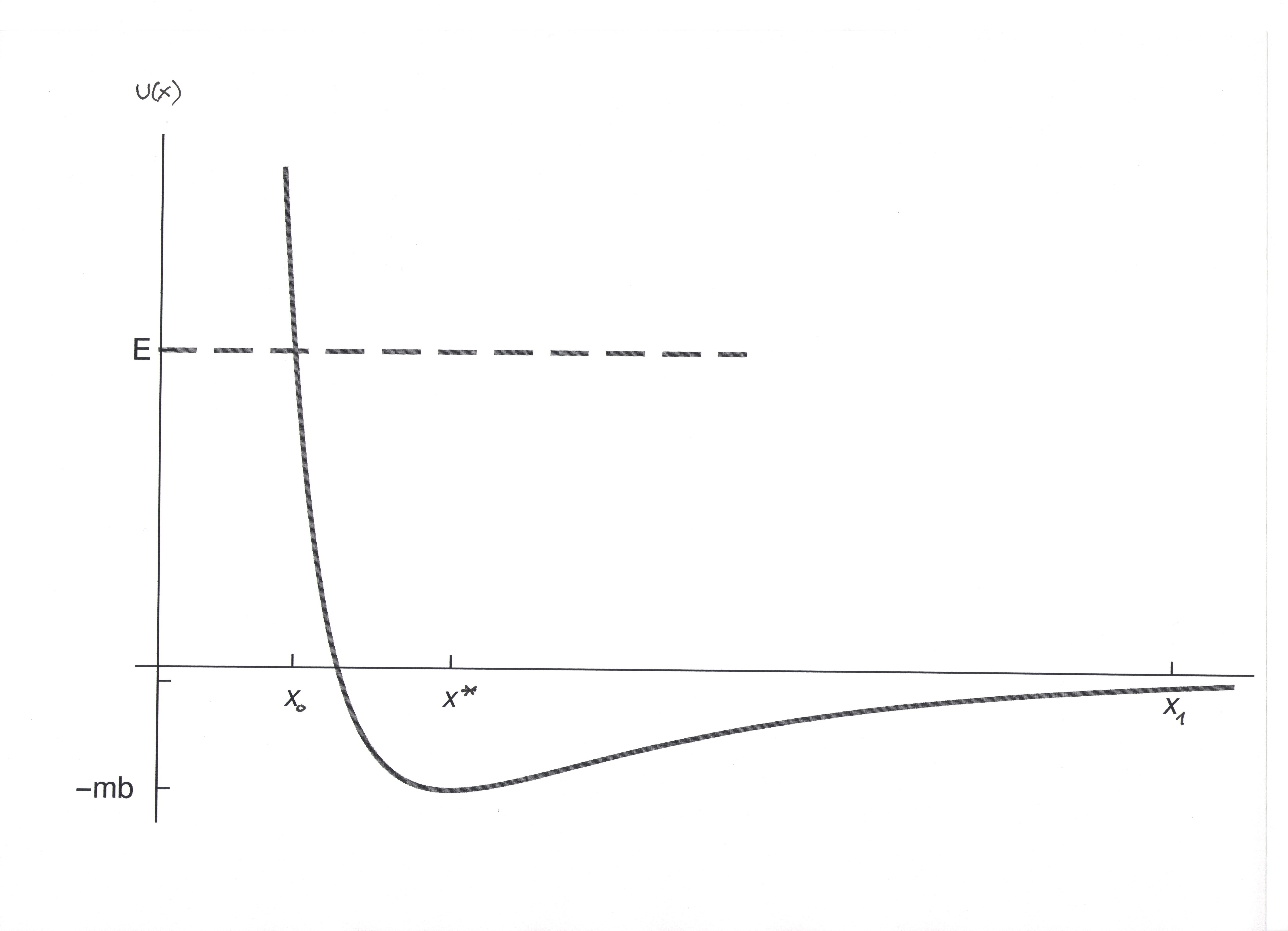
Figure 6: Potential with repulsive core. The minimum of the potential ($-mb$) is at $x=x^{*}$. For the calculation of the time delay the motion between the turning point $x_{o}$ and a distant point $x_{1}$ is used.

The formula for the time delay for scattering processes is given by

$$\Delta(E)=-\sqrt{2m}\left\{\frac{\xi_{1}(E)}{\sqrt{E}}+\int_{0}^{E}\xi_{1}^{\prime}(U){\rm d}U\left[\frac{1}{\sqrt{E-U}}-\frac{1}{\sqrt{E}}\right]+\int_{0}^{mb}d^{\prime}(V){\rm d}V\left[\frac{1}{\sqrt{E+V}}-\frac{1}{\sqrt{E}}\right]\right\}.$$ (62)

It depends on $\xi_{1}(U)$ and $d(V)$, i.e. on both inverse functions $\xi_{1}$, $\xi_{2}$. Using the LL trick, we can express $\xi_{1}(U)$ for $U\geq 0$ as

$$\xi_{1}(U)=-\frac{1}{\pi\sqrt{2m}}\int_{0}^{U}\frac{\Delta(E){\rm d}E}{\sqrt{U-E}}-\frac{1}{\pi}\sqrt{U}\int_{0}^{mb}d(V)\frac{{\rm d}V}{\sqrt{V}(U+V)}.$$ (63)

We see that this still depends on the width function. The scattering data alone are not enough to find both inverse functions and reconstruct the potential. For this we also need to consider the bound state problem (see Fig. 7). First we have to calculate the half-period of periodic motions with negative energy $E=-\varepsilon<0$:

$$\tilde{T}(\varepsilon)=\sqrt{\frac{m}{2}}\int_{y_{1}}^{y_{2}}\frac{{\rm d}x}{\sqrt{-\varepsilon-U(x)}}=-\sqrt{\frac{m}{2}}\int_{\varepsilon}^{mb}d^{\prime}(V)\frac{{\rm d}V}{\sqrt{V-\varepsilon}}.$$ (64)

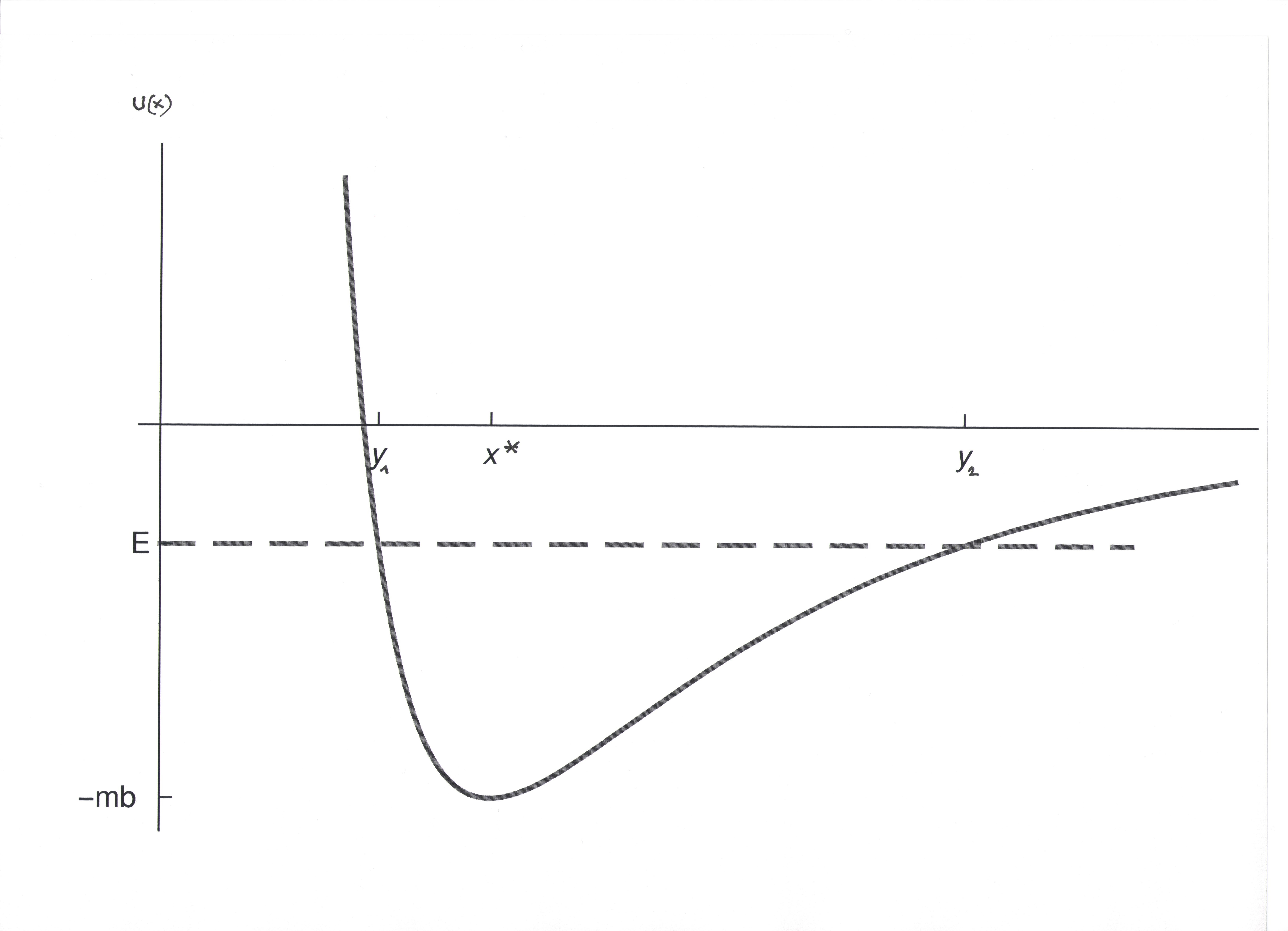
Figure 7: Bound motion in an RC type potential. For negative total energy $E$ the turning points are $y_{1}$ and $y_{2}$.

Now we can use the LL-trick to determine the width function:

$$d(V)=\frac{1}{\pi}\sqrt{\frac{2}{m}}\int_{V}^{mb}\frac{\tilde{T}(\varepsilon){\rm d}\varepsilon}{\sqrt{\varepsilon-V}}.$$ (65)

Finally, using this result in (63) we can reconstruct $\xi_{1}$ in terms of scattering and bound state data:

$$\xi_{1}(U)=-\frac{1}{\pi\sqrt{2m}}\int_{0}^{U}\frac{\Delta(E){\rm d}E}{\sqrt{U-E}}-\frac{1}{\pi}\sqrt{\frac{2}{m}}\int_{0}^{mb}\frac{\tilde{T}(\varepsilon){\rm d}\varepsilon}{\sqrt{\varepsilon+U}}.$$ (66)

A.4 Localized attractive potential (LA)

The last example we discuss is shown in Fig 8. For simplicity, here we discuss a symmetric, attractive potential, which takes its minimum value, $-mb$, at the origin. Here we can define the functional inverse $\xi(U)$ for $x\geq 0$. We assume $U(\infty)=0$ again. There are scattering and bound motions and we can calculate the time delay for $E>0$:

$$\Delta(E)=\sqrt{2m}\int_{0}^{mb}\xi^{\prime}(-V){\rm d}V\left[\frac{1}{\sqrt{E+V}}-\frac{1}{\sqrt{E}}\right],$$ (67)

and also the half-period of bound motions for $E=-\varepsilon<0$:

$$\tilde{T}(\varepsilon)=\sqrt{2m}\int_{\varepsilon}^{mb}\xi^{\prime}(-V)\frac{{\rm d}V}{\sqrt{V-\varepsilon}}.$$ (68)

This last result is already enough to reconstruct the inverse potential by the LL-trick:

$$\xi(-V)=\frac{1}{\pi\sqrt{2m}}\int_{V}^{mb}\frac{\tilde{T}(\varepsilon){\rm d}\varepsilon}{\sqrt{\varepsilon-V}}.$$ (69)

The scattering time delay is determined by the same function and is not independent. We find that there is a constraint between the time delay and the half-period:

$$\Delta(E)=-\frac{1}{\pi\sqrt{E}}\int_{0}^{mb}\frac{\tilde{T}(\varepsilon)\sqrt{\varepsilon}{\rm d}\varepsilon}{\varepsilon+E}.$$ (70)

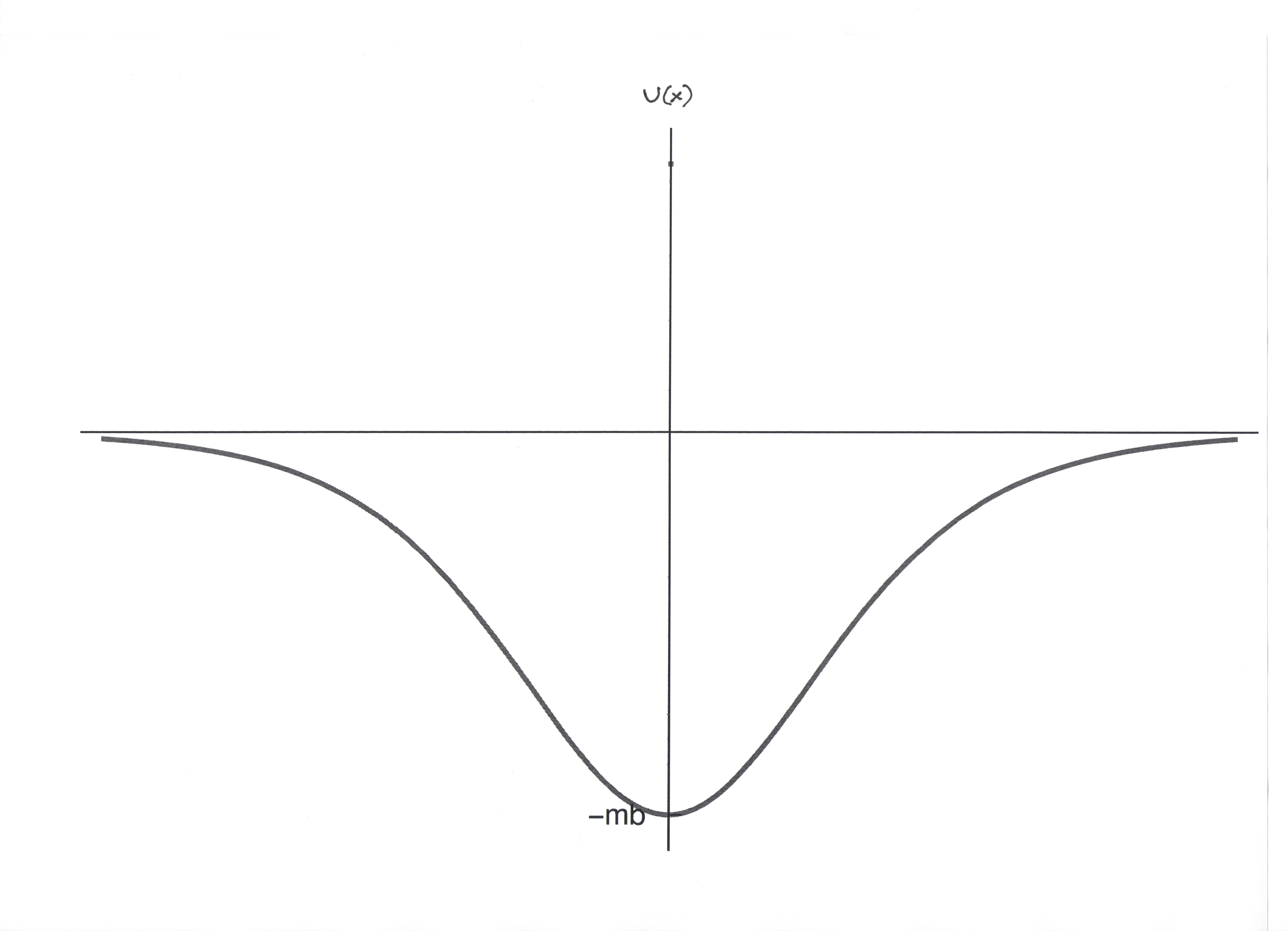
Figure 8: Localized attractive potential. Both scattering and bound motions are possible.

A.5 Space-time picture of scattering

For repulsive scattering (MR and RC cases) the space-time diagram of the process is depicted in Fig. 9. The free motion in the asymptotic past is given by

$$x(t)\approx x^{(-)}(t)=-vt+a,\qquad\qquad t\to-\infty$$ (71)

and in the asymptotic future

$$x(t)\approx x^{(+)}(t)=vt+b,\qquad\qquad t\to+\infty.$$ (72)

The values of the constants $a$, $b$ depend on the arbitrary choice of the origin of the time coordinate, but their sum is uniquely determined by the asymptotic velocity $v$, i.e. the energy of the process. An alternative definition of the time delay is

$$x^{(+)}(t+\Delta)=-x^{(-)}(t).$$ (73)

It is given by

$$\Delta=-\frac{a+b}{v}.$$ (74)

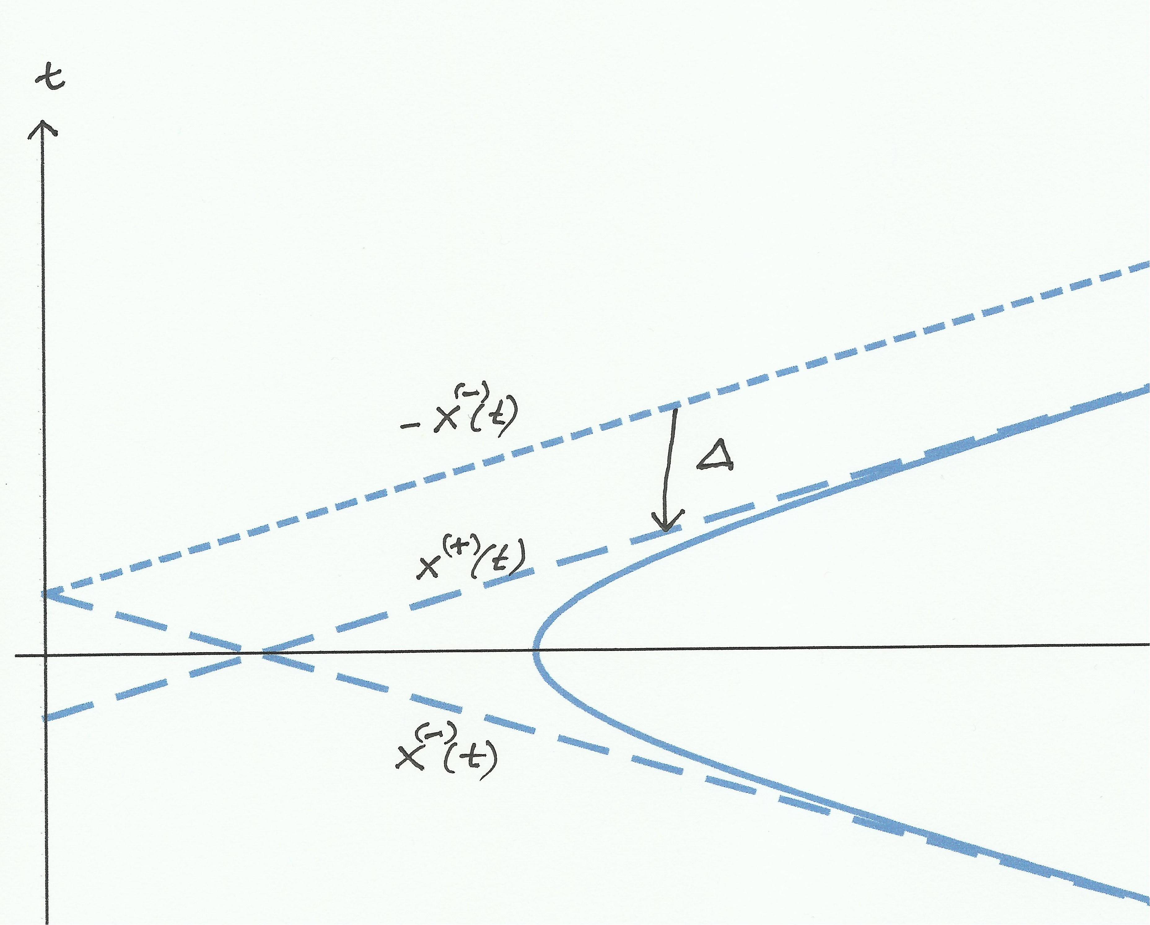
Figure 9: Space-time diagram of a particle scattering off a potential. The time shift between the actual asymptotic motion and the free motion after bouncing back at the origin is the time delay.

Similarly, for the scattering process in the LA case

$$x^{(-)}(t)=vt+a,\qquad\qquad x^{(+)}(t)=vt+b,\qquad\qquad$$ (75)

$$x^{(+)}(t+\Delta)=x^{(-)}(t),\qquad\qquad\Delta=\frac{a-b}{v}.$$ (76)

A.6 Two-particle problem

Let us scale out the mass $m$ from the one-particle problem introducing $W(x)$ by

$$U(x)=mW(x).$$ (77)

Let us further introduce the notations

$$\tau([W];v)=\Delta,\qquad\qquad T_{o}(h)=\tilde{T}(mh)\quad(E=-mh<0).$$ (78)

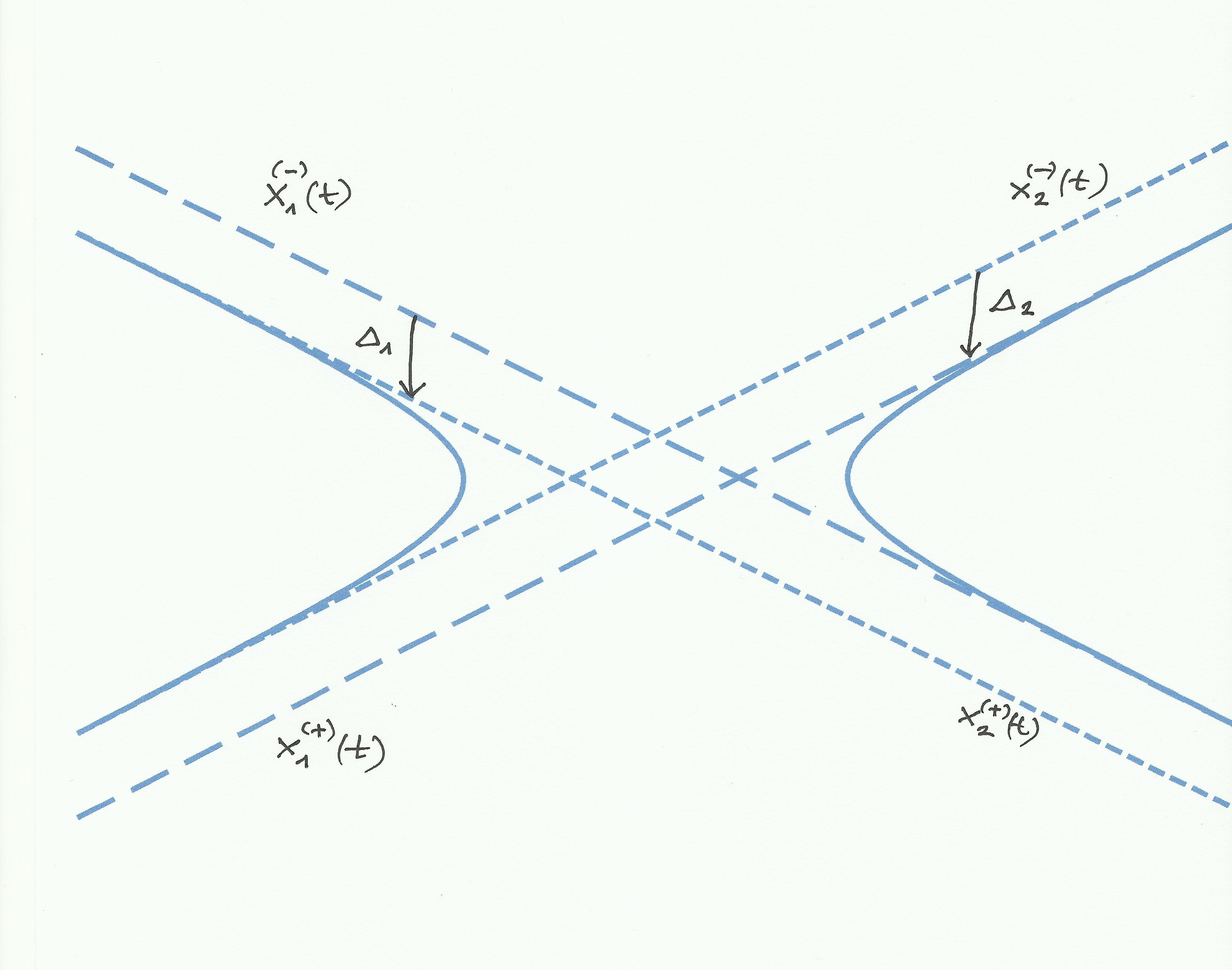
Figure 10: Space-time diagram of a repulsive two-particle scattering process. The time shift between the actual final asymptotics and the extrapolation of the initial asymptotics is the time delay.

The simple exercises we have discussed in the previous subsections can be applied to the study of 2-particle problems. Assuming that the particles are both of mass $m$ and interact through the potential $U(x_{1}-x_{2})$, we can write down the equations of motion:

$$m\ddot{x}_{1}=-U^{\prime}(x_{1}-x_{2}),\qquad\qquad m\ddot{x}_{2}=U^{\prime}(x_{1}-x_{2}).$$ (79)

As is well known, introducing the relative coordinate

$$y(t)=x_{1}(t)-x_{2}(t)$$ (80)

we can reduce the problem to an effective 1-particle one

$$m\ddot{y}=-2U^{\prime}(y)$$ (81)

with the same potential, but reduced mass $m/2$.

Let us now consider the case of repulsive scattering (Fig. 10). Because the scattering is elastic, the asymptotic velocities are swapped:

$$\begin{split}t\to-\infty:\qquad\quad x_{i}(t)&\approx x_{i}^{(-)}(t)=v_{i}t+a_{i},\qquad\qquad v_{\underline{1}}=v_{2},\\ t\to+\infty:\qquad\quad x_{i}(t)&\approx x_{i}^{(+)}(t)=v_{\underline{i}}t+b_{i},\qquad\qquad v_{\underline{2}}=v_{1}.\end{split}$$ (82)

The time delays are determined by

$$x_{2}^{(+)}(t+\Delta_{1})=x_{1}^{(-)}(t),\qquad\qquad\Delta_{1}=\frac{a_{1}-b_{2}}{v_{1}}$$ (83)

and

$$x_{1}^{(+)}(t+\Delta_{2})=x_{2}^{(-)}(t),\qquad\qquad\Delta_{2}=\frac{a_{2}-b_{1}}{v_{2}}.$$ (84)

The kinematics is somewhat simplified in the COM frame. Here $x_{1}(t)+x_{2}(t)=0$ and

$$-v_{1}=v_{2}=v,\qquad\qquad a_{2}=-a_{1},\qquad b_{2}=-b_{1}.$$ (85)

The time delays are equal:

$$\Delta_{1}=\Delta_{2}=-\frac{a_{1}+b_{1}}{v}=T(v).$$ (86)

For the relative motion we have

$$y^{(-)}(t)=-2vt+2a_{1},\qquad\quad y^{(+)}(t)=2vt+2b_{1},$$ (87)

i.e. we have to consider an effective one-particle problem with (mass-reduced) potential $2W$ and asymptotic velocity $2v$. We can calculate the time delay $\Delta$ in this effective problem and find

$$\Delta=\tau([2W];2v)=-\frac{2a_{1}+2b_{1}}{2v}=-\frac{a_{1}+b_{1}}{v}=T(v).$$ (88)

The case of attractive scattering is very similar. We define

$$t\to\pm\infty\qquad\quad x_{i}(t)\approx x_{i}^{(\pm)}(t)=v_{i}t+\left\{\begin{aligned} &b_{i}\\ &a_{i}\end{aligned}\right.$$ (89)

and

$$x_{i}^{(+)}(t+\Delta_{i})=x_{i}^{(-)}(t),\qquad\qquad\Delta_{i}=\frac{a_{i}-b_{i}}{v_{i}}.$$ (90)

Again, in the COM frame the kinematics simplifies:

$$v_{1}=-v_{2}=v,\qquad a_{2}=-a_{1},\quad b_{2}=-b_{1},\qquad\Delta_{1}=\Delta_{2}=\frac{a_{1}-b_{1}}{v}=T(v).$$ (91)

For the effective one-particle problem we have

$$y^{(-)}(t)=2vt+2a_{1},\qquad y^{(+)}(t)=2vt+2b_{1}$$ (92)

and for the time delay $\Delta$

$$\Delta=\tau([2W];2v)=\frac{2a_{1}-2b_{1}}{2v}=\frac{a_{1}-b_{1}}{v}=T(v).$$ (93)

A.7 Scaling properties

Let us denote the solution of the equations of motion with (mass reduced) potential $W(x)$ by $x(t)$. It is the solution of

$$\ddot{x}(t)=-W^{\prime}(x(t)).$$ (94)

If we rescale the time variable by a constant $\lambda$ we can define

$$z(t)=x(\lambda t).$$ (95)

It solves

$$\ddot{z}(t)=-\lambda^{2}W^{\prime}(z(t)),$$ (96)

i.e. it is the solution of the equations of motion with potential $\lambda^{2}W(x)$. We have seen that for repulsive scattering the asymptotics is given by

$$x^{(-)}(t)=-vt+a,\qquad\quad x^{(+)}(t)=vt+b$$ (97)

and the time delay is

$$\tau([W];v)=-\frac{a+b}{v}.$$ (98)

After rescaling we have

$$z^{(-)}(t)=-v\lambda t+a,\qquad\quad z^{(+)}(t)=v\lambda t+b$$ (99)

and

$$\tau([\lambda^{2}W];\lambda v)=-\frac{a+b}{\lambda v}=\frac{1}{\lambda}\tau([W];v).$$ (100)

The same scaling rule holds also for attractive scattering.

The time delay in the two-particle problem in the COM frame is

$$T(v)=\tau([2W];2v)=\frac{1}{\sqrt{2}}\tau([W];\sqrt{2}v).$$ (101)

Here we have used the scaling rule with $\lambda=\sqrt{2}$, $v\rightarrow\sqrt{2}v$.

Later we will see that the formulas become simpler if we use instead of the time delay $T(v)$ the space displacement

$$X(v)=-vT(v).$$ (102)

We have defined it with a minus sign because it turns out that in all our examples the time delay is actually negative (which means that the interacting particles move faster than the free ones).

For bound states in the original problem with half-period $T_{o}(h)$ we have

$$x(t+2T_{o})=x(t).$$ (103)

Here $-h$ is the conserved (mass-reduced) one-particle energy

$$-h=\frac{1}{2}\dot{x}^{2}(t)+W(x(t)).$$ (104)

If we denote by $P$ the full period of the time-rescaled motion we have

$$z(t+P)=z(t).$$ (105)

This gives $\lambda P=2T_{o}$ and for the two-particle case in the COM frame ($\lambda=\sqrt{2}$)

$$P=\sqrt{2}T_{o}.$$ (106)

The (mass-reduced) two-particle energy is

$$\frac{1}{2}\dot{x}_{1}^{2}(t)+\frac{1}{2}\dot{x}_{2}^{2}(t)+W(x_{1}(t)-x_{2}(t))=\frac{1}{4}\dot{y}^{2}(t)+W(y(t))=\frac{1}{2}\dot{x}^{2}(\sqrt{2}t)+W(x(\sqrt{2}t))=-h,$$ (107)

i.e. it is the same as the corresponding one-particle energy. Thus we have simply

$$P(h)=\sqrt{2}T_{o}(h)=\sqrt{2}\tilde{T}(mh),\qquad\quad E=-mh<0.$$ (108)

A.8 Simplified inverse formulas

Using the new variables $X(v)$ (displacement in the COM frame) and $P(h)$ (full period of bound motion with total COM energy $E=-mh$) the inverse formulas are simplified and can be written as follows.

MR type potential:

$$\xi(mW)=\frac{2}{\pi}\int_{0}^{\pi/2}X(\sqrt{W}\sin\varphi){\rm d}\varphi.$$ (109)

RC type potential:

$$\xi_{1}(mW)=\frac{2}{\pi}\int_{0}^{\pi/2}X(\sqrt{W}\sin\varphi){\rm d}\varphi-\frac{1}{\pi}\int_{0}^{b}\frac{P(h){\rm d}h}{\sqrt{h+W}},$$ (110)

$$d(m{\cal V})=\frac{1}{\pi}\int_{\cal V}^{b}\frac{P(h){\rm d}h}{\sqrt{h-{\cal V}}}.$$ (111)

LA type potential:

$$\xi(-m{\cal V})=\frac{1}{2\pi}\int_{\cal V}^{b}\frac{P(h){\rm d}h}{\sqrt{h-{\cal V}}}.$$ (112)

In the LA case we also have a constraint and the displacement can be expressed with the period:

$$X(v)=\frac{1}{2\pi}\int_{0}^{b}{\rm d}h\,\frac{P(h)\sqrt{h}}{h+v^{2}}.$$ (113)

A.9 Examples

For MR type potentials we take the example

$$U(x)=\frac{mg^{2}}{\sinh^{2}(x/\ell)},$$ (114)

where $g$ is a constant with dimension of velocity and $\ell$ is the unit of length. The inverse function is

$$\xi(U)=\ell\,{\rm arcsinh}\left(\sqrt{\frac{mg^{2}}{U}}\right).$$ (115)

For this example the scattering data can be computed analytically and we find

$$X(v)=\frac{\ell}{2}\ln\left(1+\frac{g^{2}}{v^{2}}\right).$$ (116)

For the LA case we take the example

$$U(x)=-\frac{mg^{2}}{\cosh^{2}(x/\ell)},$$ (117)

$$\xi(U)=\ell\,{\rm arccosh}\left(\sqrt{-\frac{mg^{2}}{U}}\right).$$ (118)

The scattering data are

$$P(h)=\frac{\ell\pi}{\sqrt{h}},\qquad\qquad X(v)=\frac{\ell}{2}\ln\left(1+\frac{g^{2}}{v^{2}}\right).$$ (119)

We see that the displacement is exactly the same for the two above cases.

For RC type potentials (see Fig. 6) we take

$$U(x)=mB\,\frac{\xi-{\rm e}^{x/\ell}}{({\rm e}^{x/\ell}-1)^{2}},$$ (120)

where $B>0$ is a constant with dimension ${\rm velocity}^{2}$, $\ell$ is the length unit and $\xi>1$ is a dimensionless constant.

For small $x$

$$U(x)\approx\frac{m\ell^{2}B(\xi-1)}{x^{2}}$$ (121)

and for large $x$

$$U(x)\approx-mB{\rm e}^{-x/\ell}.$$ (122)

The potential vanishes at $x=\ell\ln\xi$ and its minimum is at $x=x^{*}=\ell\ln(2\xi-1)$:

$$U(x^{*})=-mb=-\frac{mB}{4(\xi-1)}.$$ (123)

The two partial inverse functions are

$$\xi_{1}(U)=\ell g_{1}\left(\frac{U}{mB}\right),\qquad\qquad\xi_{2}(U)=\ell g_{2}\left(\frac{U}{mB}\right),$$ (124)

where

$$g_{1}(\omega)=\ln\frac{2(\omega-\xi)}{2\omega-1-\sqrt{1+4\omega(\xi-1)}},\qquad\quad\omega\geq-\frac{1}{4(\xi-1)},$$ (125)

$$g_{2}(\omega)=\ln\frac{2(\omega-\xi)}{2\omega-1+\sqrt{1+4\omega(\xi-1)}},\qquad\quad 0\geq\omega\geq-\frac{1}{4(\xi-1)}.$$ (126)

Again, the scattering data can be calculated analytically:

$$P(h)=\frac{\ell\pi}{\sqrt{h}}-\frac{\ell\pi}{\sqrt{h+B\xi}},$$ (127)

$$X(v)=\ell\hat{X}\left(\frac{v}{\sqrt{B}}\right)$$ (128)

with

$$\begin{split}\hat{X}(u)&=\ln\frac{2u^{2}-1+\sqrt{1+4k}}{2\xi-1+\sqrt{1+4k}}+\ln\frac{1+4k+\sqrt{1+4k}}{8u^{4}}\\ &+\frac{u}{\sqrt{u^{2}-\xi}}\left(\ln\frac{1+\alpha_{1}\sqrt{u^{2}-\xi}}{1-\alpha_{1}\sqrt{u^{2}-\xi}}+\ln\frac{1+\alpha_{2}\sqrt{u^{2}-\xi}}{1-\alpha_{2}\sqrt{u^{2}-\xi}}\right),\end{split}$$ (129)

where

$$\alpha_{1}=\frac{1}{u(2\xi-1)},\qquad\alpha_{2}=\frac{\sqrt{1+4k}-1}{u(\sqrt{1+4k}+2\xi-1)},\qquad k=u^{2}(\xi-1).$$ (130)

Note that $\hat{X}(u)$ is real for all $u>0$, for $u^{2}<\xi$ we can use the identity

$$\frac{1}{\sqrt{u^{2}-\xi}}\ln\left(\frac{1+\alpha\sqrt{u^{2}-\xi}}{1-\alpha\sqrt{u^{2}-\xi}}\right)=\frac{2}{\sqrt{\xi-u^{2}}}\arctan(\alpha\sqrt{\xi-u^{2}}).$$ (131)

A.10 Large distance and low energy asymptotics

A.10.1 MR type potentials

Let us assume that (as in our examples) the inverse function can be expanded for small $U$ (which corresponds to large $\xi$) as

$$\xi(U)=-{\cal L}\ln\frac{U}{mu_{o}^{2}}+\left[\hat{\alpha}+\hat{\beta}\ln\frac{U}{mu_{o}^{2}}\right]\frac{U}{mu_{o}^{2}}+\dots,$$ (132)

where ${\cal L}$, $u_{o}$ and $\hat{\alpha},\ \hat{\beta}$ are constants and the neglected terms are higher powers of $U$ with coefficients that are polynomials in $\ln\frac{U}{mu_{o}^{2}}$. In this case the low energy expansion of the scattering displacement is of the form

$$X(v)={\cal L}\ln\frac{u_{o}^{2}}{4v^{2}}+\frac{2v^{2}}{u_{o}^{2}}\left[\hat{\alpha}+\hat{\beta}\left(\ln\frac{4v^{2}}{u_{o}^{2}}-1\right)\right]+\dots$$ (133)

plus higher terms in $v^{2}$ with logarithmic coefficients. The relation between the two expansions is perturbative (also for the higher terms). In our $1/\sinh^{2}$ example

$${\cal L}=\frac{\ell}{2},\qquad u_{o}=2g,\qquad\hat{\alpha}=\ell,\qquad\hat{\beta}=0.$$ (134)

A.10.2 LA type potentials

Here we assume an expansion of the form

$$\xi(-V)=-{\cal L}\ln\frac{V}{mu_{o}^{2}}+{\rm O}(V).$$ (135)

The corresponding low energy expansion of the scattering data is

$$P(h)=\frac{2\pi{\cal L}}{\sqrt{h}}+p_{o}+{\rm O}(\sqrt{h}),\qquad\quad X(v)={\cal L}\ln\frac{u_{o}^{2}}{4v^{2}}-\frac{vp_{o}}{2}+{\rm O}(v^{2}),$$ (136)

where the constant $p_{o}$ is non-perturbative and is given by the formula

$$p_{o}=-\left\{\frac{4{\cal L}}{\sqrt{b}}-2\sqrt{m}\int_{0}^{mb}\frac{{\rm d}V}{\sqrt{V}}\left[\xi^{\prime}(-V)-\frac{{\cal L}}{V}\right]\right\}.$$ (137)

In our $-1/\cosh^{2}$ example

$${\cal L}=\frac{\ell}{2},\qquad u_{o}=2g,\qquad p_{o}=0.$$ (138)

A.10.3 RC type potentials

We assume that

$$\xi_{2}(-V)=-{\cal L}\ln\frac{V}{mu_{o}^{2}}+{\rm O}(V),\qquad\quad\xi_{1}(0)={\cal L}z_{o}.$$ (139)

The corresponding low energy expansion of the scattering data is

$$P(h)=\frac{\pi{\cal L}}{\sqrt{h}}+p_{o}+{\rm O}(\sqrt{h}),\qquad\quad X(v)={\cal L}\ln\frac{u_{o}^{2}}{4v^{2}}-vp_{o}+{\rm O}(v^{2}).$$ (140)

The non-perturbative constant $p_{o}$ is given by the formula

$$p_{o}=-\left\{\frac{2{\cal L}}{\sqrt{b}}+\sqrt{m}\int_{0}^{mb}\frac{{\rm d}V}{\sqrt{V}}\left[d^{\prime}(V)+\frac{{\cal L}}{V}\right]\right\}.$$ (141)

In our RC example

$${\cal L}=\ell,\qquad u_{o}^{2}=B,\qquad z_{o}=\ln\xi,\qquad p_{o}=-\frac{\ell\pi}{\sqrt{B\xi}}.$$ (142)

References

- [1] N. Ishii, S. Aoki and T. Hatsuda, The nuclear force from lattice QCD, Phys. Rev. Lett. 99, 022001 (2007) [arXiv:nucl-th/0611096].
- [2] S. Aoki, T. Hatsuda and N. Ishii, Nuclear Force from Monte Carlo Simulations of Lattice Quantum Chromodynamics, Comput. Sci. Dis. 1, 015009 (2008) [arXiv:0805.2462 [hep-ph]].
- [3] S. Aoki, T. Hatsuda and N. Ishii, Theoretical Foundation of the Nuclear Force in QCD and its applications to Central and Tensor Forces in Quenched Lattice QCD Simulations, Prog. Theor. Phys. 123, 89(2010) [arXiv:0909.5585 [hep-lat]].
- [4] N. Ishizuka, PoS LAT2009, 119 (2009).
- [5] T. Inoue et al. [HAL QCD collaboration], Baryon-Baryon Interactions in the Flavor SU(3) Limit from Full QCD Simulations on the Lattice, Prog. Theor. Phys. 124, 591 (2010) [arXiv:1007.3559 [hep-lat]].
- [6] T. Inoue et al. [HAL QCD Collaboration], Phys. Rev. Lett. 106, 162002(2011) Bound H-dibaryon in Flavor SU(3) Limit of Lattice QCD, [ arXiv:1012.5928 [hep-lat]].
- [7] T. Doi, S. Aoki, T. Hatsuda, Y. Ikeda, T. Inoue, N. Ishii, K. Murano and H. Nemura et al., Exploring Three-Nucleon Forces in Lattice QCD, Prog. Theor. Phys. 127, 723 (2012) [arXiv:1106.2276 [hep-lat]].
- [8] S. Aoki, J. Balog and P. Weisz, Application of the operator product expansion to the short distance behavior of nuclear potentials, JHEP05, 008 (2010) [arXiv:1002.0977 [hep-lat]].
- [9] S. Aoki, J. Balog and P. Weisz, The repulsive core of the NN potential and the operator product expansion, PoS LAT2009, 132 (2009) [arXiv:0910.4255 [hep-lat]].
- [10] S. Aoki, J. Balog and P. Weisz, Operator product expansion and the short distance behavior of 3-flavor baryon potentials, JHEP09, 083 (2010) [arXiv:1007.4117 [hep-lat]].
- [11] S. Aoki, J. Balog and P. Weisz, Short distance repulsion in 3 nucleon forces from perturbative QCD, New J. Phys. 14 (2012) 043046 [arXiv:1112.2053 [hep-lat]].
- [12] S. Aoki, J. Balog and P. Weisz, Toward an understanding of short distance repulsions among baryons in QCD – NBS wave functions and operator product expansion –, Prog. Theor. Phys. 128, 1269 (2012) [arXiv:1208.1530 [hep-lat]].
- [13] S. Aoki, J. Balog and P. Weisz, Bethe-Salpeter wave functions in integrable models, Prog. Theor. Phys. 121 (2009) 1003 [arXiv:0805.3098 [hep-th]].
- [14] S. N. M. Ruijsenaars and H. Schneider, A New Class of Integrable Systems and Its Relation to Solitons, Annals Phys. 170 (1986) 370.
- [15] S. N. M. Ruijsenaars, Sine-Gordon solitons versus relativistic Calogero-Moser particles, Proceedings, NATO Advanced Research Workshop on dynamical symmetries of integrable quantum field theories and lattice models, Kiev, Ukraine, September 25-30, 2000, (NATO ASI series II: Mathematics, physics and chemistry. 35)
- [16] J. Balog, Relativistic trajectory variables in 1+1 dimensional Ruijsenaars-Schneider type models, arXiv:1402.6990 [hep-th].
- [17] L. D. Landau, E. M. Lifshitz, Mechanics (Course of Theoretical Physics, Volume 1) §12.