Fractionally integrated inverse stable subordinators

Abstract

A fractionally integrated inverse stable subordinator (FIISS) is the convolution of a power function and an inverse stable subordinator. We show that the FIISS is a scaling limit in the Skorokhod space of a renewal shot noise process with heavy-tailed, infinite mean ‘inter-shot’ distribution and regularly varying response function. We prove local Hölder continuity of FIISS and a law of iterated logarithm for both small and large times.

2010 Mathematics Subject Classification: Primary 60F17, 60G17
2010 Mathematics Subject Classification: Secondary 60G18

Keywords: Hölder continuity; inverse stable subordinator; Lamperti representation; law of iterated logarithm; renewal shot noise process; self-similarity; weak convergence in the Skorokhod space

1 Introduction

1.1 A brief survey of inverse stable subordinators

For $\alpha\in(0,1)$, let $(D_{\alpha}(t))_{t\geq 0}$ be an $\alpha$-stable subordinator, i.e., an increasing Lévy process, with $-\log\mathbb{E}e^{-tD_{\alpha}(1)}=\Gamma(1-\alpha)t^{\alpha}$ for $t\geq 0$, where $\Gamma(\cdot)$ is Euler’s gamma function. Its generalized inverse $W_{\alpha}:=(W_{\alpha}(u))_{u\in\mathbb{R}}$ defined by

$$W_{\alpha}(u)~{}:=~{}\inf\{t\geq 0:D_{\alpha}(t)>u\},\quad u\geq 0$$

and $W_{\alpha}(u):=0$ for $u<0$, is called an inverse $\alpha$-stable subordinator. Obviously, $W_{\alpha}$ has a.s. continuous and nondecreasing sample paths. Further, it is clear that $W_{\alpha}$ is self-similar with index $\alpha$, i.e., the finite-dimensional distributions of $(W_{\alpha}(cu))_{u\geq 0}$ for fixed $c>0$ are the same as those of $(c^{\alpha}W_{\alpha}(u))_{u\geq 0}$.

More specific properties of $W_{\alpha}$ include (local) Hölder continuity with arbitrary exponent $\gamma<\alpha$ which is a consequence of

$$M:=\sup_{0\leq v<u\leq 1/2}\,\frac{W_{\alpha}(u)-W_{\alpha}(v)}{(u-v)^{\alpha}|\log(u-v)|^{1-\alpha}}<\infty\quad\text{a.s.}$$ (1)

(Lemma 3.4 in [33]), a modulus of continuity result

$$\underset{\delta\to 0+}{\lim}\,\underset{\begin{subarray}{c}0\leq t\leq 1\\ 0<h<\delta\end{subarray}}{\sup}\,\frac{W_{\alpha}(t+h)-W_{\alpha}(t)}{h^{\alpha}|\log h|^{1-\alpha}}=\frac{1}{\Gamma(1-\alpha)\alpha^{2\alpha-1}(1-\alpha)^{1-\alpha}}\quad\text{a.s.}$$

(formula (6) in [12]), and the law of iterated logarithm

$$\lim\sup\,\frac{W_{\alpha}(u)}{u^{\alpha}(\log|\log u|)^{1-\alpha}}=\frac{1}{\Gamma(1-\alpha)\alpha^{\alpha}(1-\alpha)^{1-\alpha}}\quad\text{a.s.}$$ (2)

both as $u\to 0+$ and $u\to+\infty$ which can be extracted from Theorem 4.1 in [3]. For later needs, we note that the random variable $M$ defined in (1) satisfies

$$\mathbb{E}e^{sM}<\infty$$ (3)

for all $s>0$ (Lemma 3.4 in [33]).

Denote by $D[0,\infty)$ and $D(0,\infty)$ the Skorokhod spaces of right-continuous real-valued functions which are defined on $[0,\infty)$ and $(0,\infty)$, respectively, and have finite limits from the left at each positive point. Elements of these spaces are sometimes called càdlàg functions. Throughout the paper, weak convergence on $D[0,\infty)$ or $D(0,\infty)$ endowed with the well-known $J_{1}$-topology is denoted by $\Rightarrow$. See [5, 39] for a comprehensive account on the $J_{1}$-topology.

Let $\xi_{1}$, $\xi_{2},\ldots$ be a sequence of independent copies of a positive random variable $\xi$. Denote by $(S_{n})_{n\in\mathbb{N}_{0}}$, where $\mathbb{N}_{0}:=\mathbb{N}\cup\{0\}$, the zero-delayed standard random walk with jumps $\xi_{k}$, i.e., $S_{0}:=0$ and $S_{n}:=\xi_{1}+\ldots+\xi_{n}$ for $n\in\mathbb{N}$. The corresponding first-passage time process is defined by

$$\nu(t):=\inf\{k\in\mathbb{N}_{0}:S_{k}>t\},\quad t\in\mathbb{R}.$$

Note that $\nu(t)=0$ for $t<0$.

Assume that

$$\mathbb{P}\{\xi>t\}\quad\sim\quad t^{-\alpha}\ell(t),\quad t\to\infty$$ (4)

for some $\alpha\in(0,1)$ and some $\ell$ slowly varying at $\infty$. Then, according to Corollary 3.4 in [30],

$$\mathbb{P}\{\xi>t\}\nu(ut)\quad\Rightarrow\quad W_{\alpha}(u),\quad t\to\infty$$ (5)

on $D[0,\infty)$.

In the recent years inverse stable subordinators, also known as Mittag-Leffler processes, have become a popular object of research, both from the theoretical and applied viewpoints. Relation (5) which tells us that the processes $W_{\alpha}$ are scaling limits of the first-passage time processes with heavy-tailed waiting times underlies the ubiquity of inverse stable subordinators in a heavy-tailed world. For instance, inverse stable subordinators are often used as a time-change of the subordinated processes intended to model heavy-tailed phenomena. The most prominent example of this kind is a scaling limit for continuous-time random walks with heavy-tailed waiting times [30, 31]. In the simplest situation, the scaling limit takes the form $S(W_{\alpha}(\cdot))$, where $S(\cdot)$ is a $\gamma$-stable process with $0<\gamma\leq 2$. The special case $\gamma=2$ appears in many problems related to the anomalous (or fractional) diffusion and has attracted considerable attention in both physics [25, 38] and mathematics literature [2, 24, 32]. More general subordinated processes $X(W_{\alpha}(\cdot))$, with $X$ being a Markov process, can be used to construct solutions to fractional partial differential equations [28, 29]. Also, inverse stable subordinators play an important role in the analysis of (a) stationary infinitely divisible processes generated by conservative flows [11, 33] and (b) asymptotics of convolutions of certain (explicitly given) functions and rescaled continuous-time random walks [37]. In (a) and (b), the limit processes are convolutions involving inverse stable subordinators and, as such, are close relatives of processes $Y_{\alpha,\,\beta}$ to be introduced below.

1.2 Definition and known properties of fractionally integrated inverse stable subordinators

In this section we define the processes which are in focus in the present paper and review some of their known properties.

For $\beta\in\mathbb{R}$, set

$$Y_{\alpha,\,\beta}(0):=0,\quad Y_{\alpha,\,\beta}(u):=\int_{[0,\,u]}(u-y)^{\beta}{\rm d}W_{\alpha}(y),\quad u>0.$$

Since the integrator $W_{\alpha}$ has nondecreasing paths, the integral exists as a pathwise Lebesgue-Stieltjes integral. Proposition 2.6 below shows that $Y_{\alpha,\,\beta}(u)<\infty$ a.s. for each fixed $u>0$. Following [15] and [19], we call $Y_{\alpha,\,\beta}:=(Y_{\alpha,\,\beta}(u))_{u\geq 0}$ fractionally integrated inverse $\alpha$-stable subordinator.

In [15], it was shown that the processes $Y_{\alpha,\,\beta}$ with $\beta\geq 0$ are scaling limits in the Skorokhod space of renewal shot noise processes with eventually nondecreasing regularly varying response functions and heavy-tailed ‘inter-shot’ distributions of infinite mean. According to Theorem 2.9 in [19], in the case when $\beta\in[-\alpha,0]$ (and the response functions are eventually nonincreasing) a similar statement holds in the sense of weak convergence of finite-dimensional distributions. More exotic processes involving $Y_{\alpha,\,\beta}$ arise as scaling limits for random processes with immigration which are renewal shot noise processes with random response functions (see [20] for the precise definition). In Proposition 2.2 of [20], the limit is a conditionally Gaussian process with conditional variance $Y_{\alpha,\,\beta}$.

We shall use the representations

$$Y_{\alpha,\,\beta}(u)=\beta\int_{0}^{u}(u-y)^{\beta-1}W_{\alpha}(y){\rm d}y,\quad u>0$$ (6)

when $\beta>0$ and

$$Y_{\alpha,\,\beta}(u) = u^{\beta}W_{\alpha}(u)+|\beta|\int_{0}^{u}(W_{\alpha}(u)-W_{\alpha}(u-y))y^{\beta-1}{\rm d}y$$ (7)

$$= |\beta|\int_{0}^{\infty}(W_{\alpha}(u)-W_{\alpha}(u-y))y^{\beta-1}{\rm d}y,\quad u>0$$

when $-\alpha<\beta<0$. These show that $Y_{\alpha,\,\beta}$ is nothing else but the Riemann-Liouville fractional integral (up to a multiplicative constant) of $W_{\alpha}$ in the first case and the Marchaud fractional derivative of $W_{\alpha}$ in the second (see p. 33 and p. 111 in [36]).

Here are some known properties of $Y_{\alpha,\,\beta}$.

• $Y_{\alpha,\,\beta}(u)<\infty$ a.s. for each $u>0$ (the case $\beta\geq 0$ is trivial; the case $\beta\in(-\alpha,0)$ is covered by Lemma 2.14 in [18]; for arbitrary $\beta$, see Proposition 2.6 below).

• $Y_{\alpha,\,\beta}$ is a.s. continuous whenever $\beta>-\alpha$ (see p. 1993 in [15] for the case $\beta\geq 0$ and Proposition 2.18 in [18] for the case $\beta\in(-\alpha,0)$). In the case when $\beta\leq-\alpha$ the probability that $Y_{\alpha,\,\beta}$ is unbounded on a given interval is strictly positive (see the proof of Proposition 2.7 in [20] for the case $\beta=-\alpha$; although an extension to the case $\beta<-\alpha$ is straightforward, it is discussed in the proof of Proposition 2.6 below for the sake of completeness).

• The increments of $Y_{\alpha,\,\beta}$ are neither independent nor stationary (see p. 1994 in [15] and Proposition 2.16 in [18]).

• $Y_{\alpha,\,\beta}$ is self-similar with index $\alpha+\beta$ (even though this can be easily checked, we state this observation as Proposition 2.5 for ease of reference).

Three realizations of inverse $3/4$-stable subordinators together with the corresponding fractionally integrated inverse $3/4$-stable subordinators for different $\beta$ are shown on Figure 1.

$\alpha=0.75$ and $\beta=0.5$

$\alpha=0.75$ and $\beta=-0.5$

$\alpha=0.75$ and $\beta=-1.5$

Figure 1: Inverse stable subordinators (left) and the corresponding FIISS (right)

The rest of the paper is structured as follows. Main results are formulated in Section 2. Theorem 2.1 states that fractionally integrated stable subordinators $Y_{\alpha,\,\beta}$ for $\beta>-\alpha$ are scaling limits in the Skorokhod space of certain renewal shot noise processes with heavy-tailed ‘inter-shot’ distributions. Since the renewal shot noise processes are extensively used in diverse areas of applied mathematics, the processes $Y_{\alpha,\,\beta}$, as their limits, may be useful for heavy-tailed modeling. The paths of $Y_{\alpha,\,\beta}$ for $\beta\leq-\alpha$ are ill-behaved (see Proposition 2.6). Hence, the convergence of finite-dimensional distributions provided by Theorem 2.4 is the best possible result in this case. The other main results of the paper are concerned with sample path properties of $Y_{\alpha,\,\beta}$. Theorem 2.7 is a Hölder-type result which generalizes (1). Theorem 2.9 is the law of iterated logarithm for both small and large times which generalizes (2). In Section 3 we show that $Y_{\alpha,\,\beta}(1)$ has the same distribution as the exponential functional of a killed subordinator by exploiting the Lamperti representation [22] of semi-stable processes. The main results are proved in Sections 4, 5 and 6. The Appendix collects several auxiliary results.

2 Main results

2.1 Fractionally integrated inverse stable subordinators as scaling limits of renewal shot noise processes

Below we shall use the notation introduced in Section 1.1.

For a càdlàg function $h$, define

$$X(t):=\sum_{k\geq 0}h(t-S_{k})\operatorname{\mathbbm{1}}_{\{S_{k}\leq t\}}=\int_{[0,\,t]}h(t-y){\rm d}\nu(y),\quad t\geq 0.$$

The process $(X(t))_{t\geq 0}$ is called renewal shot noise process with response function $h$. There has been an outbreak of recent activity around weak convergence of renewal shot noise processes and their generalizations called random processes with immigration, see [1, 15, 17, 19, 20, 21]. Both renewal shot noise processes and random processes with immigration are ubiquitous in applied mathematics. Many relevant references can be traced via the last cited articles.

Theorem 2.1.

Assume that $\mathbb{P}\{\xi>t\}\sim t^{-\alpha}\ell(t)$ for some $\alpha\in(0,1)$ and some $\ell$ slowly varying at $\infty$. Let $h:[0,\infty)\to[0,\infty)$ be a right-continuous monotone function that satisfies $h(t)\sim t^{\beta}\widehat{\ell}(t)$ for some $\beta>-\alpha$ and some $\widehat{\ell}$ slowly varying at $\infty$. Then, as $t\to\infty$,

$$\frac{\mathbb{P}\{\xi>t\}}{h(t)}\sum_{k\geq 0}h(ut-S_{k})\operatorname{\mathbbm{1}}_{\{S_{k}\leq ut\}}\quad\Rightarrow\quad Y_{\alpha,\,\beta}(u)$$

on $D(0,\infty)$.

Remark 2.2.

In the case $\beta\geq 0$, Theorem 2.1 was proved in [15] under weaker assumptions that $h:[0,\infty)\to\mathbb{R}$ is càdlàg, eventually nondecreasing and regularly varying. In Section 4 we shall show that, in the case $\beta\leq 0$, Theorem 2.1 holds whenever $h:[0,\infty)\to\mathbb{R}$ is càdlàg, eventually nonincreasing and regularly varying.

Recall that convergence to a continuous limit in $D(0,\infty)$ equipped with the $J_{1}$-topology is equivalent to uniform convergence on $[a,b]$ for any finite positive $a$ and $b$, $a<b$. Since the limit process in Theorem 2.1 has a.s. continuous sample paths we obtain the following

Corollary 2.3.

Under the assumptions of Theorem 2.1, as $t\to\infty$,

$$\frac{\mathbb{P}\{\xi>t\}}{h(t)}\underset{u\in[a,\,b]}{\sup}\,\sum_{k\geq 0}h(ut-S_{k})\operatorname{\mathbbm{1}}_{\{S_{k}\leq ut\}}\quad\overset{d}{\to}\quad\underset{u\in[a,\,b]}{\sup}\,Y_{\alpha,\,\beta}(u)$$

for any finite positive $a$ and $b$, $a<b$.

Extremal behavior of shot-noise processes has attracted considerable attention in the literature, see [7, 13, 14, 23, 26, 27]. However, assumptions of the cited papers were other than ours.

By Proposition 2.6 below, the paths of $Y_{\alpha,\beta}$ for $\beta\leq-\alpha$ do not belong to the space $D(0,\infty)$. Although this shows that the classical functional limit theorem cannot hold, we still have the convergence of finite-dimensional distributions.

Theorem 2.4.

Under the same assumptions as in Theorem 2.1 but with arbitrary $\beta\in\mathbb{R}$ we have, as $t\to\infty$,

$$\frac{\mathbb{P}\{\xi>t\}}{h(t)}\bigg{(}\sum_{k\geq 0}h(u_{1}t-S_{k})\operatorname{\mathbbm{1}}_{\{S_{k}\leq u_{1}t\}},\ldots,\sum_{k\geq 0}h(u_{n}t-S_{k})\operatorname{\mathbbm{1}}_{\{S_{k}\leq u_{n}t\}}\bigg{)}\overset{d}{\to}(Y_{\alpha,\,\beta}(u_{1}),\ldots,Y_{\alpha,\,\beta}(u_{n}))$$

for any $n\in\mathbb{N}$ and any $0<u_{1}<\ldots<u_{n}<\infty$.

Since $t\mapsto\mathbb{P}\{\xi>t\}/h(t)$ varies regularly at $\infty$ with index $-\alpha-\beta$, the following statement is immediate.

Proposition 2.5.

$Y_{\alpha,\,\beta}$ is self-similar with index $\alpha+\beta$.

2.2 Sample path properties of fractionally integrated inverse stable subordinators

Our first result shows that when $\beta\leq-\alpha$ the sample paths of $Y_{\alpha,\,\beta}$ are rather irregular.

Proposition 2.6.

Assume that $\beta\leq-\alpha$. Then the random variable $Y_{\alpha,\,\beta}(u)$ is almost surely finite for any fixed $u\geq 0$. However, for every interval $I\subset(0,\infty)$ we have $\sup_{u\in I}Y_{\alpha,\,\beta}(u)=+\infty$ with positive probability. Furthermore, with probability one there exist infinitely many (random) points $u>0$ such that $Y_{\alpha,\beta}(u)=+\infty$.

The next theorem is a Hölder-type result which generalizes (1).

Theorem 2.7.

Suppose $\alpha+\beta\in(0,1)$. Then

$$\sup_{0\leq v<u\leq 1/2}\,\frac{|Y_{\alpha,\,\beta}(u)-Y_{\alpha,\,\beta}(v)|}{(u-v)^{\alpha+\beta}|\log(u-v)|^{1-\alpha}}<\infty\quad\text{a.s.}$$ (8)

Suppose $\alpha+\beta=1$. Then

$$\sup_{0\leq v<u\leq 1/2}\,\frac{Y_{\alpha,\,\beta}(u)-Y_{\alpha,\,\beta}(v)}{(u-v)|\log(u-v)|^{2-\alpha}}<\infty\quad\text{a.s.}$$ (9)

In particular, in both cases above $Y_{\alpha,\,\beta}$ is a.s. (locally) Hölder continuous with arbitrary exponent $\gamma<\alpha+\beta$. Suppose $\alpha+\beta>1$. Then

$$\sup_{0\leq v<u\leq 1/2}\,\frac{Y_{\alpha,\,\beta}(u)-Y_{\alpha,\,\beta}(v)}{u-v}<\infty\quad\text{a.s.}$$ (10)

which means that $Y_{\alpha,\,\beta}$ is a.s. (locally) Lipschitz continuous.

Remark 2.8.

In the case $\alpha+\beta>1$ the process $Y_{\alpha\,\beta}$ is actually not only a.s. locally Lipschitz continuous, but also $[\alpha+\beta]$-times continuously differentiable on $[0,\infty)$ a.s. This follows from the equality

$$Y_{\alpha,\,\beta}(u)=\beta\int_{0}^{u}Y_{\alpha,\,\beta-1}(v){\rm d}v,\quad u\geq 0$$

which shows that if $Y_{\alpha,\,\beta-1}$ is continuous, then $Y_{\alpha,\,\beta}$ is continuously differentiable.

We proceed with the law of iterated logarithm both for small and large times.

Theorem 2.9.

Whenever $\beta>-\alpha$ we have

$$\lim\sup\,\frac{Y_{\alpha,\,\beta}(u)}{u^{\alpha+\beta}(\log|\log u|)^{1-\alpha}}=\frac{1}{\Gamma(1-\alpha)(\alpha+\beta)^{\alpha}(1-\alpha)^{1-\alpha}}=:c_{\alpha,\,\beta}\quad\text{a.s.}$$ (11)

and

$$\lim\inf\,\frac{Y_{\alpha,\,\beta}(u)}{u^{\alpha+\beta}(\log|\log u|)^{1-\alpha}}=0\quad\text{a.s.}$$ (12)

both as $u\to 0+$ and $u\to+\infty$.

3 Distributional properties of the fractionally integrated inverse stable subordinators

Consider a family of processes $X_{\alpha}^{(u)}(t):=((u^{1/\alpha}-D_{\alpha}(t))^{\alpha})_{0\leq t<W_{\alpha}(u^{1/\alpha})}$ indexed by the initial value $u>0$. This family forms a semi-stable Markov process of index $1$, i.e.

$$\mathbb{P}\{cX_{\alpha}^{(u)}(t/c)\in\cdot\}=\mathbb{P}\{X_{\alpha}^{(cu)}(t)\in\cdot\}$$

for all $c>0$. Then, according to Theorem 4.1 in [22], with $u$ fixed

$$(u^{1/\alpha}-D_{\alpha}(t))^{\alpha}=u\exp(-Z_{\alpha}(\tau(t/u)))\quad\text{for}\quad 0\leq t\leq uI\quad\text{a.s.}$$

for some killed subordinator $Z_{\alpha}:=(Z_{\alpha}(t))_{t\geq 0}=(Z_{\alpha}^{(u)}(t))_{t\geq 0}$ where

$$I:=\int_{0}^{\infty}\exp(-Z_{\alpha}(t)){\rm d}t=u^{-1}\inf\{v:D_{\alpha}(v)>u^{1/\alpha}\}=u^{-1}W_{\alpha}(u^{1/\alpha})$$ (13)

and $\tau(t):=\inf\{s:\int_{0}^{s}\exp(-Z_{\alpha}(v)){\rm d}v\geq t\}$ for $0\leq t\leq I$ (except in one place, we suppress the dependence of $Z_{\alpha}$, $I$ and $\tau(t)$ on $u$ for notational simplicity). With this at hand

$$Y_{\alpha,\,\beta}(u^{1/\alpha}) = \int_{0}^{\infty}((u^{1/\alpha}-D_{\alpha}(t))^{\alpha})^{\beta/\alpha}\operatorname{\mathbbm{1}}_{\{D_{\alpha}(t)\leq u^{1/\alpha}\}}{\rm d}t$$

$$= u^{\beta/\alpha}\int_{0}^{uI}\exp(-(\beta/\alpha)Z_{\alpha}(\tau(t/u))){\rm d}t=u^{1+\beta/\alpha}\int_{0}^{I}\exp(-(\beta/\alpha)Z_{\alpha}(\tau(t))){\rm d}t$$

$$= u^{1+\beta/\alpha}\int_{0}^{\infty}\exp(-(1+\beta/\alpha)Z_{\alpha}(t)){\rm d}t.$$

Replacing $u$ with $u^{\alpha}$ we infer

$$Y_{\alpha,\,\beta}(u)=u^{\alpha+\beta}\int_{0}^{\infty}\exp(-cZ^{(u^{\alpha})}_{\alpha}(t)){\rm d}t\quad\text{a.s.}$$ (14)

where $c:=\alpha^{-1}(\alpha+\beta)$. The latter integral is known as an exponential functional of subordinator. We shall show that $Z_{\alpha}$ is a drift-free killed subordinator with the unit killing rate and the Lévy measure

$$\nu_{\alpha}({\rm d}x)=\frac{e^{-x/\alpha}}{(1-e^{-x/\alpha})^{\alpha+1}}\operatorname{\mathbbm{1}}_{(0,\,\infty)}(x){\rm d}x.$$

Equivalently, the Laplace exponent of $Z_{\alpha}$ equals

$$\Phi_{\alpha}(s):=-\log\mathbb{E}e^{-sZ_{\alpha}(1)}=1+\int_{[0,\infty)}(1-e^{-st})\nu_{\alpha}({\rm d}x)=\frac{\Gamma(1-\alpha)\Gamma(1+\alpha s)}{\Gamma(1+\alpha(s-1))},\quad s\geq 0$$

where $\Gamma(\cdot)$ is the gamma function.

It is well known that $W_{\alpha}(1)$ has a Mittag-Leffler distribution with parameter $\alpha$. This distribution is uniquely determined by its moments

$$\mathbb{E}(W_{\alpha}(1))^{n}=\frac{n!}{(\Gamma(1-\alpha))^{n}\Gamma(1+n\alpha)},\quad n\in\mathbb{N}.$$

Using (13) along with self-similarity of $W_{\alpha}$ we conclude that $I$ has the same Mittag-Leffler distribution. It follows that the moments of $I$ can be written as

$$\mathbb{E}I^{n}=\frac{n!}{(\Gamma(1-\alpha))^{n}\Gamma(1+n\alpha)}=\frac{n!}{\Phi_{\alpha}(1)\cdot\ldots\cdot\Phi_{\alpha}(n)},\quad n\in\mathbb{N}$$

which, by Theorem 2 in [4], implies that the Lévy measure of $Z_{\alpha}$ has the form as stated above.

By Lemma 7.1, $Y_{\alpha,\,\beta}(1)$ has a bounded and nonincreasing density $f_{\alpha,\,\beta}$, say. Since

$$\Psi_{\alpha,\,\beta}(s):=-\log\mathbb{E}e^{-scZ_{\alpha}(1)}=\frac{\Gamma(1-\alpha)\Gamma((\alpha+\beta)s+1)}{\Gamma((\alpha+\beta)s+1-\alpha)},\quad s\geq 0$$

and hence

$$\Psi_{\alpha,\,\beta}(s)\quad\sim\quad\Gamma(1-\alpha)(\alpha+\beta)^{\alpha}s^{\alpha},\quad s\to\infty,$$

another application of Lemma 7.1 allows us to conclude that

$$-\log\mathbb{P}\{Y_{\alpha,\,\beta}(1)>x\} \sim -\log f_{\alpha,\,\beta}(x)\sim(1-\alpha)((\alpha+\beta)^{\alpha}\Gamma(1-\alpha))^{(1-\alpha)^{-1}}x^{(1-\alpha)^{-1}}$$ (15)

$$= (x/c_{\alpha,\,\beta})^{(1-\alpha)^{-1}},\quad x\to\infty$$

with $c_{\alpha,\,\beta}$ as defined in (11). In particular, for any $\delta_{1}\in(0,1)$ there exists $c_{1}=c_{1}(\delta_{1})$ such that

$$f_{\alpha,\,\beta}(x)\leq c_{1}\exp\big{(}-(1-\delta_{1})(x/c_{\alpha,\,\beta})^{(1-\alpha)^{-1}}\big{)}$$ (16)

for all $x\geq 0$.

4 Proofs of Theorems 2.1 and 2.4, and Remark 2.2

Proof of Theorems 2.1 and 2.4.

In the case where $\beta\geq 0$ and $h$ is nondecreasing the result was proved in Theorem 1.1 of [15]. Therefore, we only investigate the case where $\beta\leq 0$ and $h$ is nonincreasing. In what follows, all unspecified limits are assumed to hold as $t\to\infty$.

Set $a(t):=\mathbb{P}\{\xi>t\}$. First we fix an arbitrary $\varepsilon\in(0,1)$ and prove that

$$I_{\varepsilon}(u,t):=\frac{a(t)}{h(t)}\sum_{k\geq 0}h(ut-S_{k})\operatorname{\mathbbm{1}}_{\{S_{k}\leq\varepsilon ut\}}\quad\Rightarrow\quad\int_{[0,\,\varepsilon u]}(u-y)^{\beta}{\rm d}W_{\alpha}(y)$$

on $D(0,\infty)$. Write

$$I_{\varepsilon}(u,t) = a(t)\sum_{k\geq 0}\bigg{(}\frac{h(ut-S_{k})}{h(t)}-(u-t^{-1}S_{k})^{\beta}\bigg{)}\operatorname{\mathbbm{1}}_{\{S_{k}\leq\varepsilon ut\}}$$

$$+ a(t)\sum_{k\geq 0}(u-t^{-1}S_{k})^{\beta}\operatorname{\mathbbm{1}}_{\{S_{k}\leq\varepsilon ut\}}$$

$$= I_{\varepsilon,\,1}(u,t)+I_{\varepsilon,\,2}(u,t).$$

We shall show that

$$I_{\varepsilon,\,1}(u,t)\quad\Rightarrow\quad r(u)\quad\text{and}\quad I_{\varepsilon,\,2}(u,t)\quad\Rightarrow\quad\int_{[0,\,\varepsilon u]}(u-y)^{\beta}{\rm d}W_{\alpha}(y)$$ (17)

on $D(0,\infty)$, where $r(u)=0$ for all $u>0$. Throughout the rest of the proof we use arbitrary positive and finite $a<b$. Observe that

$$|I_{\varepsilon,\,1}(u,t)|\leq\underset{(1-\varepsilon)u\leq y\leq u}{\sup}\,\bigg{|}\frac{h(ty)}{h(t)}-y^{\beta}\bigg{|}a(t)\nu(\varepsilon ut)$$

and thereupon

$$\underset{a\leq u\leq b}{\sup}\,|I_{\varepsilon,\,1}(u,t)|\leq\underset{(1-\varepsilon)a\leq y\leq b}{\sup}\,\bigg{|}\frac{h(ty)}{h(t)}-y^{\beta}\bigg{|}a(t)\nu(\varepsilon bt).$$

As a consequence of the functional limit theorem for $(\nu(t))_{t\geq 0}$ (see (5)), $a(t)\nu(\varepsilon bt)\overset{d}{\to}W_{\alpha}(\varepsilon b)$. This, combined with the uniform convergence theorem for regularly varying functions (Theorem 1.2.1 in [6]), implies that the last expression converges to zero in probability thereby proving the first relation in (17).

Turning to the second relation in (17) we observe that

$$I_{\varepsilon,\,2}(u,t)=\int_{[0,\,\varepsilon u]}(u-y)^{\beta}{\rm d}\left(a(t)\nu(ty)\right).$$

Recall from (5) that $a(t)\nu(ty)\Rightarrow W_{\alpha}(y)$ weakly on $D[0,\infty)$, as $t\to\infty$. Using the Skorokhod representation theorem, we can pass to versions which converge a.s. in the $J_{1}$-topology. Since the limit $W_{\alpha}$ is continuous, the a.s. convergence is even locally uniform on $[0,\infty)$. Applying Lemma 7.2 from the Appendix, we obtain the second relation in (17).

An appeal to Theorem 3.1 in [5] reveals that the proof of Theorem 2.4 is complete if we can show that for any $\beta\leq 0$ and any fixed $u>0$

$$\lim_{\varepsilon\to 1-}\int_{[0,\,\varepsilon u]}(u-y)^{\beta}{\rm d}W_{\alpha}(y)\quad=\quad Y_{\alpha,\,\beta}(u)=\int_{[0,\,u]}(u-y)^{\beta}{\rm d}W_{\alpha}(y)\quad\text{a.s.}$$ (18)

and

$$\underset{\varepsilon\to 1-}{\lim}\,\underset{t\to\infty}{\lim\sup}\,\mathbb{P}\bigg{\{}\frac{a(t)}{h(t)}\sum_{k\geq 0}h(ut-S_{k})\operatorname{\mathbbm{1}}_{\{\varepsilon ut<S_{k}\leq ut\}}>\theta\bigg{\}}=0$$ (19)

for all $\theta>0$. Analogously, Theorem 2.1 follows once we can show that for $\beta\in(-\alpha,0]$ the following two statements hold. First, the a.s. convergence in (18) is locally uniform on $(0,\infty)$. Second, a uniform analog of (19) holds, namely,

$$\underset{\varepsilon\to 1-}{\lim}\,\underset{t\to\infty}{\lim\sup}\,\mathbb{P}\bigg{\{}\frac{a(t)}{h(t)}\underset{u\in[a,\,b]}{\sup}\sum_{k\geq 0}h(ut-S_{k})\operatorname{\mathbbm{1}}_{\{\varepsilon ut<S_{k}\leq ut\}}>\theta\bigg{\}}=0$$ (20)

for all $\theta>0$.

To check that (18) holds pointwise for any $\beta\leq 0$, write for fixed $u>0$

$$0\leq\int_{[0,\,u]}(u-y)^{\beta}{\rm d}W_{\alpha}(y) - \int_{[0,\,\varepsilon u]}(u-y)^{\beta}{\rm d}W_{\alpha}(y)=\int_{[0,\,u]}(u-y)^{\beta}\operatorname{\mathbbm{1}}_{(\varepsilon u,\,u]}(y){\rm d}W_{\alpha}(y).$$

By the dominated convergence theorem, the right-hand side converges to $0$ a.s. as $\varepsilon\to 1-$ because $\int_{[0,\,u]}(u-y)^{\beta}{\rm d}W_{\alpha}(y)<\infty$ a.s. by Proposition 2.6.

The probability on the left-hand side of (19) is bounded from above by

$$\mathbb{P}\{\nu(ut)-\nu(\varepsilon ut)>0\} = \mathbb{P}\{\nu(ut)-\nu(\varepsilon ut)\geq 1\}=\mathbb{P}\{ut-S_{\nu(ut)-1}<(1-\varepsilon)ut\}.$$

By a well-known Dynkin-Lamperti result (see Theorem 8.6.3 in [6])

$$t^{-1}(t-S_{\nu(t)-1})\quad\overset{d}{\to}\quad\eta_{\alpha}$$

where $\eta_{\alpha}$ has a beta distribution with parameters $1-\alpha$ and $\alpha$, i.e.,

$$\mathbb{P}\{\eta_{\alpha}\in{\rm d}x\}=\pi^{-1}\sin(\pi\alpha)x^{-\alpha}(1-x)^{\alpha-1}\operatorname{\mathbbm{1}}_{(0,1)}(x){\rm d}x.$$

This entails

$$\underset{\varepsilon\to 1-}{\lim}\,\underset{t\to\infty}{\lim\sup}\,\mathbb{P}\{\nu(ut)-\nu(\varepsilon ut)>0\}=\underset{\varepsilon\to 1-}{\lim}\,\mathbb{P}\{\eta_{\alpha}<1-\varepsilon\}=0$$

thereby proving (19). The proof of Theorem 2.4 is complete.

Now we turn to the proof of Theorem 2.1. In particular, $\beta\in(-\alpha,0]$ is the standing assumption in what follows.

The right-hand side of (18) is a.s. continuous (see point (II) in Section 1.2). Further, it can be checked that the left-hand side of (18) is a.s. continuous, too. Since it is also monotone in $\varepsilon$ we can invoke Dini’s theorem to conclude that the a.s. convergence in (18) is locally uniform on $(0,\infty)$.

To check (20), we need the following proposition to be proved in the Appendix.

Proposition 4.1.

Fix $T>0$ and set $A_{t}:=\{(u,v):0\leq v<u\leq T,u-v\geq 1/t\}$ for $t>0$. If $a(t)=\mathbb{P}\{\xi>t\}\sim t^{-\alpha}\ell(t)$ for some $\alpha\in(0,1)$ and some $\ell$ slowly varying at $\infty$, then, for any $\delta\in(0,\alpha)$,

$$\lim_{x\to\infty}\limsup_{t\to\infty}\mathbb{P}\left\{\sup_{(u,v)\in A_{t}}\frac{a(t)(\nu(ut)-\nu(vt))}{(u-v)^{\alpha-\delta}}>x\right\}=0.$$

Fix now $\Delta\in(0,(\alpha+\beta)/2)$ and note that by Potter’s bound for regularly varying functions (Theorem 1.5.6 in [6]) there exists $c>1$ such that

$$\frac{h(t(u-y))}{h(t)}\leq 2(u-y)^{\beta-\Delta}$$

for all $t$, $u$ and $y$ such that $t(u-y)\geq c$ and $u-y\leq 1$. With this at hand, we have for $t$ large enough, $u\in[a,b]$ and $\varepsilon>0$ such that $(1-\varepsilon)b\leq 1$

$$\frac{a(t)}{h(t)}\sum_{k\geq 0}h(ut-S_{k})\operatorname{\mathbbm{1}}_{\{\varepsilon ut<S_{k}\leq ut\}}$$

$$= \frac{a(t)}{h(t)}\int_{(\varepsilon u,\,u-c/t]}h(t(u-y)){\rm d}\nu(ty)+\frac{a(t)}{h(t)}\int_{(u-c/t,\,u]}h(t(u-y)){\rm d}\nu(ty)$$

$$\leq 2a(t)\int_{(\varepsilon u,\,u-c/t]}(u-y)^{\beta-\Delta}{\rm d}\nu(ty)+\frac{a(t)}{h(t)}h(0)(\nu(tu)-\nu(tu-c))$$

$$= 2(-\beta+\Delta)\int_{\varepsilon u}^{u-c/t}a(t)(\nu(tu)-\nu(ty))(u-y)^{\beta-\Delta-1}{\rm d}y$$

$$+ 2u^{\beta-\Delta}(1-\varepsilon)^{\beta-\Delta}a(t)(\nu(tu)-\nu(\varepsilon tu))$$

$$+ \bigg{(}\frac{a(t)}{h(t)}h(0)-2c^{\beta-\Delta}t^{-\beta+\Delta}a(t)\bigg{)}(\nu(tu)-\nu(tu-c)).$$

Since $t\mapsto a(t)/h(t)$ and $t\mapsto t^{-\beta+\Delta}a(t)$ are regularly varying of negative indices $-\alpha-\beta$ and $-\alpha-\beta+\Delta$, respectively, we have

$$\bigg{(}\frac{a(t)}{h(t)}h(0)-2c^{\beta-\Delta}t^{-\beta+\Delta}a(t)\bigg{)}\sup_{u\in[a,\,b]}(\nu(tu)-\nu(tu-c))\quad\overset{\mathbb{P}}{\to}\quad 0$$

by Lemma 7.3. Further,

$$\sup_{u\in[a,b]}u^{\beta-\Delta}(1-\varepsilon)^{\beta-\Delta}a(t)(\nu(tu)-\nu(\varepsilon tu))\leq a^{\beta-\Delta}(1-\varepsilon)^{\beta-\Delta}a(t)\sup_{u\in[a,\,b]}(\nu(tu)-\nu(\varepsilon tu))$$

and

$$a(t)\sup_{u\in[a,\,b]}(\nu(tu)-\nu(\varepsilon tu))\quad\overset{d}{\to}\quad\underset{u\in[a,\,b]}{\sup}\,(W_{\alpha}(u)-W_{\alpha}(\varepsilon u))$$

in view of (5) and the continuous mapping theorem. Therefore,

$$\lim_{\varepsilon\to 1-0}\limsup_{t\to\infty}\mathbb{P}\left\{\sup_{u\in[a,b]}u^{\beta-\Delta}(1-\varepsilon)^{\beta-\Delta}a(t)(\nu(tu)-\nu(\varepsilon tu))>\theta\right\}$$

$$\leq \lim_{\varepsilon\to 1-0}\mathbb{P}\left\{a^{\beta-\Delta}(1-\varepsilon)^{\beta-\Delta}\sup_{u\in[a,b]}(W_{\alpha}(u)-W_{\alpha}(u\varepsilon))>\theta\right\}$$

$$= \lim_{\varepsilon\to 1-0}\mathbb{P}\left\{a^{\beta-\Delta}(1-\varepsilon)^{\beta-\Delta}(2b)^{\alpha}\sup_{u\in[a/2b,1/2]}(W_{\alpha}(u)-W_{\alpha}(u\varepsilon))>\theta\right\}=0$$

for all $\theta>0$, where the penultimate equality is a consequence of self-similarity of $W_{\alpha}$, and the last equality is implied by (1) and the choice of $\Delta$.

Hence, (20) follows if we can show that

$$\underset{\varepsilon\to 1-}{\lim}\,\underset{t\to\infty}{\lim\sup}\,\mathbb{P}\left\{\sup_{u\in[0,T]}\int_{\varepsilon u}^{u-c/t}a(t)(\nu(tu)-\nu(ty))(u-y)^{\beta-\Delta-1}{\rm d}y>\theta\right\}=0$$ (21)

for all $\theta>0$ and all $T>0$. With $0<\delta<\alpha+\beta-\Delta$ the following inequality holds:

$$\mathbb{P}\left\{\sup_{u\in[0,T]}\int_{\varepsilon u}^{u-c/t}a(t)(\nu(tu)-\nu(ty))(u-y)^{\beta-\Delta-1}{\rm d}y>\theta\right\}$$

$$=\mathbb{P}\left\{\cdots,\sup_{(u,v)\in A_{t}}\frac{a(t)(\nu(ut)-\nu(vt))}{(u-v)^{\alpha-\delta}}>x\right\}+\mathbb{P}\left\{\cdots,\sup_{(u,v)\in A_{t}}\frac{a(t)(\nu(ut)-\nu(vt))}{(u-v)^{\alpha-\delta}}\leq x\right\}$$

$$\leq\mathbb{P}\left\{\sup_{(u,v)\in A_{t}}\frac{a(t)(\nu(ut)-\nu(vt))}{(u-v)^{\alpha-\delta}}>x\right\}+\mathbb{P}\left\{\sup_{u\in[0,T]}\int_{\varepsilon u}^{u}(u-y)^{\alpha+\beta-\Delta-\delta-1}{\rm d}y>\delta/x\right\}$$

$$=\mathbb{P}\left\{\sup_{(u,v)\in A_{t}}\frac{a(t)(\nu(ut)-\nu(vt))}{(u-v)^{\alpha-\delta}}>x\right\}+\mathbb{P}\left\{\int_{0}^{(1-\varepsilon)T}y^{\alpha+\beta-\Delta-\delta-1}{\rm d}y>\delta/x\right\}$$

for $x>0$. Sending $t\to\infty$ and then $\varepsilon\to 1-$ and $x\to\infty$ and using Proposition 4.1 for the first summand on the right-hand side finishes the proof of (21). The proof of Theorem 2.1 is complete. ∎

Proof of Remark 2.2.

Let $h:[0,\infty)\to\mathbb{R}$ be a càdlàg function which is nonincreasing on $[d,\infty)$ for some $d>0$ and satisfies $h(t)\sim t^{\beta}\widehat{\ell}(t)$ for some $\beta\in(-\alpha,0]$ as $t\to\infty$. Further, let $h^{\ast}:[0,\infty)\to[0,\infty)$ be any right-continuous nonincreasing function such that $h^{\ast}(t)=h(t)$ for $t\geq d$.

Then, for any positive and finite $a<b$,

$$\underset{u\in[a,\,b]}{\sup}\,\bigg{|}\sum_{k\geq 0}h(ut-S_{k})\operatorname{\mathbbm{1}}_{\{S_{k}\leq ut\}}-\sum_{k\geq 0}h^{\ast}(ut-S_{k})\operatorname{\mathbbm{1}}_{\{S_{k}\leq ut\}}\bigg{|}$$

$$\leq \underset{u\in[a,\,b]}{\sup}\,\sum_{k\geq 0}\big{|}h(ut-S_{k})-h^{\ast}(ut-S_{k})\big{|}\operatorname{\mathbbm{1}}_{\{ut-d<S_{k}\leq ut\}}$$

$$\leq \underset{y\in[0,\,d]}{\sup}\,|h(y)-h^{\ast}(y)|\underset{u\in[a,\,b]}{\sup}\,(\nu(ut)-\nu(ut-d)).$$

The normalization $\mathbb{P}\{\xi>t\}/h(t)$ used in Theorem 2.1 is regularly varying of index $-\alpha-\beta$ which is negative in the present situation. This implies that, as $t\to\infty$, the right-hand side of the last centered formula multiplied by $\mathbb{P}\{\xi>t\}/h(t)$ converges to zero in probability by Lemma 7.3 which justifies Remark 2.2. ∎

5 Proofs of Proposition 2.6 and Theorem 2.7

Proof of Proposition 2.6.

Let $\mathcal{R}$ be the range of subordinator $D_{\alpha}$ defined by

$$\mathcal{R}:=\{t>0:\text{ there exists }y>0\text{ such that }D_{\alpha}(y)=t\}.$$

If $u\notin\mathcal{R}$, then

$$Y_{\alpha,\,\beta}(u)=\int_{[0,\,u]}(u-y)^{\beta}{\rm d}W_{\alpha}(y)=\int_{[0,\,D_{\alpha}(W_{\alpha}(u)-)]}(u-y)^{\beta}{\rm d}W_{\alpha}(y)$$

because $W_{\alpha}$ takes a constant value on $(D_{\alpha}(W_{\alpha}(u)-),u]$ and $D_{\alpha}(W_{\alpha}(u)-)<u$. This shows that $Y_{\alpha,\,\beta}(u)<\infty$ for all $u\notin\mathcal{R}$. For each fixed $u>0$ we have $\mathbb{P}\{u\in\mathcal{R}\}=0$ (see Propostion 1.9 in [3]) whence $Y_{\alpha,\,\beta}(u)<\infty$ a.s.

The proof of unboundedness goes along the same lines as that of Proposition 2.7 in [20]. Recall that $\beta<-\alpha<0$ and that $I$ is a fixed interval $[c,d]$, say. Pick arbitrary positive $a<b$ and note that

$$\mathbb{P}\{[D_{\alpha}(a),\,D_{\alpha}(b)]\subset[c,d]\}=\mathbb{P}\{c\leq D_{\alpha}(a)<D_{\alpha}(b)\leq d\}>0.$$

Let us now check that

$$\sup_{u\in[D_{\alpha}(a),\,D_{\alpha}(b)]}Y_{\alpha,\,\beta}(u)=\infty\quad\text{a.s.},$$ (22)

thereby showing that $\sup_{u\in I}Y_{\alpha,\,\beta}(u)=+\infty$ with positive probability.

According to Theorem 2 in [9], there exists an event $\Omega^{\prime}$ with $\mathbb{P}\{\Omega^{\prime}\}=1$ such that for any $\omega\in\Omega^{\prime}$

$$\limsup_{y\to s-}\frac{D_{\alpha}(s,\omega)-D_{\alpha}(y,\omega)}{(s-y)^{1/\alpha}}\leq r$$ (23)

for some deterministic constant $r\in(0,\infty)$ and some $s:=s(\omega)\in[a,\,b]$. Fix any $\omega\in\Omega^{\prime}$. There exists $s_{1}:=s_{1}(\omega)$ such that

$$\big{(}D_{\alpha}(s,\omega)-D_{\alpha}(y,\omega)\big{)}^{\beta}\geq(s-y)^{\beta/\alpha}r^{\beta}/2$$

whenever $y\in(s_{1},s)$. Set $u:=u(\omega)=D_{\alpha}(s,\omega)$ and write

$$Y_{\alpha,\,\beta}(u) = \int_{[0,\,u(\omega)]}(u(\omega)-y)^{\beta}\,{\rm d}W_{\alpha}(y,\omega)=\int_{[0,\,D_{\alpha}(s,\,\omega)]}(D_{\alpha}(s,\omega)-y)^{\beta}\,{\rm d}W_{\alpha}(y,\omega)$$

$$= \int_{0}^{s}\big{(}D_{\alpha}(s,\omega)-D_{\alpha}(y,\omega)\big{)}^{\beta}\,{\rm d}y\geq\int_{s_{1}}^{s}\big{(}D_{\alpha}(s,\omega)-D_{\alpha}(y,\omega)\big{)}^{\beta}\,{\rm d}y$$

$$\geq 2^{-1}r^{\beta}\int_{s_{1}}^{s}(s-y)^{\beta/\alpha}\,{\rm d}y~{}=~{}+\infty.$$

Since $u(\omega)\in[D_{\alpha}(a),\,D_{\alpha}(b)]$ for all $\omega\in\Omega^{\prime}$, we obtain (22).

Clearly, there are infinitely many positive $s$ such that (23) holds. Hence, $Y_{\alpha,\,\beta}(u)=+\infty$ for infinitely many $u>0$ a.s. The proof of Proposition 2.6 is complete. ∎

Our proof of Theorem 2.7 will be pathwise, hence deterministic, in the following sense. In view of (1), there exists an event $\Omega_{1}$ with $\mathbb{P}\{\Omega_{1}\}=1$ such that $M=M(\omega)<\infty$ for all $\omega\in\Omega_{1}$. Below we shall work with fixed but arbitrary $\omega\in\Omega_{1}$.

From the very beginning we want to stress that local Hölder continuity follows immediately from Theorem 3.1 on p. 53 and Lemma 13.1 on p. 239 in [36] when $\beta>0$ and $-\alpha<\beta<0$, respectively. However, proving (8) and (9) requires additional efforts.

Proof of Theorem 2.7.

Observe that

$$W_{\alpha}(x)-W_{\alpha}(y)\leq M(x-y)^{\alpha}|\log(x-y)|^{1-\alpha}$$ (24)

whenever $-\infty<y<x\leq 1/2$. This is trivial when $x\leq 0$ and is a consequence of (1) when $y\geq 0$. Assume that $y\leq 0<x$. Then $W_{\alpha}(x)-W_{\alpha}(y)=W_{\alpha}(x-y+y)\leq W_{\alpha}(x-y)\leq M(x-y)^{\alpha}|\log(x-y)|^{1-\alpha}$, where the penultimate inequality is implied by monotonicity, and the last follows from (1).

When $\beta=0$, inequality (8) reduces to (1). We shall treat the other cases separately.

Case $-\alpha<\beta<0$. Let $1/2\geq u>v>0$. Using (7) we have

$$|\beta|^{-1}|Y_{\alpha,\,\beta}(u)-Y_{\alpha,\,\beta}(v)|$$

$$= \bigg{|}\int_{0}^{\infty}(W_{\alpha}(u)-W_{\alpha}(u-y)-W_{\alpha}(v)+W_{\alpha}(v-y))y^{\beta-1}{\rm d}y\bigg{|}$$

$$\leq \int_{0}^{u-v}(W_{\alpha}(u)-W_{\alpha}(u-y))y^{\beta-1}{\rm d}y+\int_{0}^{u-v}(W_{\alpha}(v)-W_{\alpha}(v-y))y^{\beta-1}{\rm d}y$$

$$+ \int_{u-v}^{\infty}(W_{\alpha}(u)-W_{\alpha}(v))y^{\beta-1}{\rm d}y+\int_{u-v}^{\infty}(W_{\alpha}(u-y)-W_{\alpha}(v-y))y^{\beta-1}{\rm d}y$$

$$\leq 2M\bigg{(}\int_{0}^{u-v}y^{\alpha+\beta-1}|\log y|^{1-\alpha}{\rm d}y+(u-v)^{\alpha}|\log(u-v)|^{1-\alpha}\int_{u-v}^{\infty}y^{\beta-1}{\rm d}y\bigg{)}$$

$$= 2M\bigg{(}\int_{0}^{u-v}y^{\alpha+\beta-1}|\log y|^{1-\alpha}{\rm d}y+|\beta|^{-1}(u-v)^{\alpha+\beta}|\log(u-v)|^{1-\alpha}\bigg{)}$$

having utilized (24) for the last inequality. Further,

$$\int_{0}^{u-v}y^{\alpha+\beta-1}|\log y|^{1-\alpha}{\rm d}y = (u-v)^{\alpha+\beta}\int_{0}^{1}t^{\alpha+\beta-1}|\log(u-v)+\log t|^{1-\alpha}{\rm d}t$$ (25)

$$\leq (u-v)^{\alpha+\beta}|\log(u-v)|^{1-\alpha}\int_{0}^{1}t^{\alpha+\beta-1}{\rm d}t$$

$$+ (u-v)^{\alpha+\beta}\int_{0}^{1}t^{\alpha+\beta-1}|\log t|^{1-\alpha}{\rm d}t$$

$$\leq \bigg{(}\frac{1}{\alpha+\beta}+\frac{\int_{0}^{1}t^{\alpha+\beta-1}|\log t|^{1-\alpha}{\rm d}t}{(\log 2)^{1-\alpha}}\bigg{)}(u-v)^{\alpha+\beta}|\log(u-v)|^{1-\alpha}$$

$$=: \kappa_{\alpha,\,\beta}(u-v)^{\alpha+\beta}|\log(u-v)|^{1-\alpha}.$$

Thus, we have proved that

$$|Y_{\alpha,\,\beta}(u)-Y_{\alpha,\,\beta}(v)|\leq 2M(|\beta|\kappa_{\alpha,\beta}+1)(u-v)^{\alpha+\beta}|\log(u-v)|^{1-\alpha}$$ (26)

whenever $1/2\geq u>v>0$.

The proof for the case $1/2\geq u>v=0$ proceeds similarly but simpler and starts with the equality

$$Y_{\alpha,\,\beta}(u)-Y_{\alpha,\,\beta}(0)=Y_{\alpha,\,\beta}(u)=u^{\beta}W_{\alpha}(u)+|\beta|\int_{0}^{u}(W_{\alpha}(u)-W_{\alpha}(u-y))y^{\beta-1}{\rm d}y.$$

The resulting estimate is

$$Y_{\alpha,\,\beta}(u)\leq M(|\beta|\kappa_{\alpha,\beta}+1)u^{\alpha+\beta}|\log u|^{1-\alpha}$$ (27)

whenever $1/2\geq u>0$. Combining (26) and (27) proves (8).

Case $\beta>0$. Let $1/2\geq u>v\geq 0$. Then $Y_{\alpha,\,\beta}(u)\geq Y_{\alpha,\,\beta}(v)$. Setting $I(u,v):=\int_{[0,\,v]}((u-y)^{\beta}-(v-y)^{\beta}){\rm d}W_{\alpha}(y)$ we obtain

$$Y_{\alpha\,\,\beta}(u)-Y_{\alpha,\,\beta}(v) = \int_{[0,\,v]}((u-y)^{\beta}-(v-y)^{\beta}){\rm d}W_{\alpha}(y)+\int_{(v,\,u]}(u-y)^{\beta}{\rm d}W_{\alpha}(y)$$ (28)

$$\leq I(u,v)+(u-v)^{\beta}(W_{\alpha}(u)-W_{\alpha}(v))$$

$$\leq I(u,v)+M(u-v)^{\alpha+\beta}|\log(u-v)|^{1-\alpha}$$

where the last inequality is a consequence of (24).

Subcase $\beta\geq 1$. We have $(u-y)^{\beta}-(v-y)^{\beta}\leq\beta(u-y)^{\beta-1}(u-v)\leq\beta(u-v)$ by the mean value theorem for differentiable functions. Hence $I(u,v)\leq\beta W_{\alpha}(1/2)(u-v)$. This, together with (28) and the inequality

$$x^{\alpha+\beta}|\log x|^{1-\alpha}\leq cx$$ (29)

which holds for $x\in(0,1/2]$ and some $c>0$, proves (10).

Subcase $\alpha+\beta>1$ and $0<\beta<1$. An appeal to the case $-\alpha<\beta<0$ that we have already settled allows us to conclude that $Y_{\alpha,\,\beta-1}$ is a.s. continuous on $[0,\,1/2]$ which implies

$$\sup_{v\in[0,\,1/2]}\,Y_{\alpha,\,\beta-1}(v)<\infty\quad\text{a.s.}$$

Another application of the mean value theorem yields $(u-y)^{\beta}-(v-y)^{\beta}\leq\beta(v-y)^{\beta-1}(u-v)$ and thereupon

$$I(u,v)\leq\beta(u-v)\int_{[0,v]}(v-y)^{\beta-1}{\rm d}W_{\alpha}(y)\leq\beta(u-v)\sup_{v\in[0,\,1/2]}\,Y_{\alpha,\,\beta-1}(v).$$

Recalling (28) and (29), we arrive at (10).

Subcase $\alpha+\beta\leq 1$ and $\beta>0$. We use (6) together with a decomposition given on p. 54 in [36]:

$$Y_{\alpha,\,\beta}(u)-Y_{\alpha,\,\beta}(v) = W_{\alpha}(v)(u^{\beta}-v^{\beta})-\beta\int_{0}^{u-v}(W_{\alpha}(v)-W_{\alpha}(u-y))y^{\beta-1}{\rm d}y$$

$$+ \beta\int_{0}^{v}(W_{\alpha}(v)-W_{\alpha}(v-y))(y^{\beta-1}-(y+u-v)^{\beta-1}){\rm d}y\leq I_{1}+I_{2}$$

where

$$I_{1}:=W_{\alpha}(v)(u^{\beta}-v^{\beta})\quad\text{and}\quad I_{2}:=\beta\int_{0}^{v}(W_{\alpha}(v)-W_{\alpha}(v-y))(y^{\beta-1}-(y+u-v)^{\beta-1}){\rm d}y.$$

We first obtain a preliminary estimate for $I_{2}$. Using (24), changing the variable and then using the subadditivity of $x\to x^{1-\alpha}$ we obtain

$$I_{2} \leq \beta M\int_{0}^{v}y^{\alpha}|\log y|^{1-\alpha}(y^{\beta-1}-(y+u-v)^{\beta-1}){\rm d}y$$

$$= \beta M(u-v)^{\alpha+\beta}\int_{0}^{v/(u-v)}t^{\alpha}|\log(u-v)+\log t|^{1-\alpha}(t^{\beta-1}-(t+1)^{\beta-1}){\rm d}t$$

$$\leq \beta M(u-v)^{\alpha+\beta}|\log(u-v)|^{1-\alpha}\int_{0}^{v/(u-v)}t^{\alpha}(t^{\beta-1}-(t+1)^{\beta-1}){\rm d}t$$

$$+ \beta M(u-v)^{\alpha+\beta}\int_{0}^{v/(u-v)}t^{\alpha}|\log t|^{1-\alpha}(t^{\beta-1}-(t+1)^{\beta-1}){\rm d}t.$$

Further we distinguish two cases.

Let $v\leq u-v$. Then

$$I_{2} \leq \beta M(u-v)^{\alpha+\beta}|\log(u-v)|^{1-\alpha}\int_{0}^{1}t^{\alpha+\beta-1}{\rm d}t$$

$$+ \beta M(u-v)^{\alpha+\beta}\int_{0}^{1}t^{\alpha+\beta-1}|\log t|^{1-\alpha}{\rm d}t\leq\beta M\kappa_{\alpha,\,\beta}(u-v)^{\alpha+\beta}|\log(u-v)|^{1-\alpha}$$

with $\kappa_{\alpha,\,\beta}$ defined in (25). As for $I_{1}$, we infer

$$I_{1}\leq W_{\alpha}(u-v)(u-v)^{\beta}\leq M(u-v)^{\alpha+\beta}|\log(u-v)|^{1-\alpha}$$

having utilized monotonicity of $W_{\alpha}$ and subadditivity of $x\mapsto x^{\beta}$ (observe that $\beta\in(0,1)$) for the first inequality and (24) for the second.

Let $v>u-v$. Using the inequality $x^{\beta-1}-(x+1)^{\beta-1}\leq(1-\beta)x^{\beta-2}$, $x>0$, we conclude that

$$I_{2} \leq \beta M(u-v)^{\alpha+\beta}|\log(u-v)|^{1-\alpha}\bigg{(}\int_{0}^{1}t^{\alpha+\beta-1}{\rm d}t+(1-\beta)\int_{1}^{\infty}t^{\alpha+\beta-2}{\rm d}t\bigg{)}$$

$$+ \beta M(u-v)^{\alpha+\beta}\bigg{(}\int_{0}^{1}t^{\alpha+\beta-1}|\log t|^{1-\alpha}{\rm d}t+(1-\beta)\int_{1}^{\infty}t^{\alpha+\beta-2}(\log t)^{1-\alpha}{\rm d}t\bigg{)}$$

$$\leq \zeta_{\alpha,\,\beta}\,(u-v)^{\alpha+\beta}|\log(u-v)|^{1-\alpha}$$

provided that $\alpha+\beta<1$. Here and in the next centered formula $\zeta_{\alpha,\,\beta}$ denotes an a.s. finite random variable whose value is of no importance. If $\alpha+\beta=1$, we have

$$I_{2} \leq \beta M(u-v)|\log(u-v)|^{1-\alpha}\bigg{(}1+(1-\beta)\int_{1}^{v/(u-v)}t^{-1}{\rm d}t\bigg{)}$$

$$+ \beta M(u-v)\bigg{(}\int_{0}^{1}|\log t|^{1-\alpha}{\rm d}t+(1-\beta)\int_{1}^{v/(u-v)}t^{-1}(\log t)^{1-\alpha}{\rm d}t\bigg{)}$$

$$\leq \beta M(u-v)|\log(u-v)|^{1-\alpha}(1+(1-\beta)|\log(u-v)|)$$

$$+ \beta M(u-v)\bigg{(}\int_{0}^{1}|\log t|^{1-\alpha}{\rm d}t+(1-\beta)(2-\alpha)^{-1}|\log(u-v)|^{2-\alpha}\bigg{)}$$

$$\leq \zeta_{\alpha,\,\beta}\,(u-v)|\log(u-v)|^{2-\alpha}.$$

Finally we use (24) and $(1+x)^{\beta}-1\leq\beta x$, $x\geq 0$ to obtain

$$I_{1} \leq Mv^{\alpha+\beta}|\log v|^{1-\alpha}((1+(u-v)/v)^{\beta}-1)\leq\beta Mv^{\alpha+\beta-1}|\log v|^{1-\alpha}(u-v)$$

$$\leq \beta M(u-v)^{\alpha+\beta}|\log(u-v)|^{1-\alpha}.$$

The proof of Theorem 2.7 is complete. ∎

6 Proof of Theorem 2.9

Since $Y_{\alpha,\,\beta}$ is self-similar with index $\alpha+\beta$ (see Proposition 2.5) we conclude that

$$\frac{Y_{\alpha,\,\beta}(u)}{u^{\alpha+\beta}(\log|\log u|)^{1-\alpha}}\overset{\mathbb{P}}{\to}0$$

as $u\to 0+$ or $u\to+\infty$. Taking an appropriate sequence we arrive at (12).

Turning to the upper limit we first prove that

$$\underset{u\to+\infty}{\lim\sup}\,\frac{Y_{\alpha,\,\beta}(u)}{u^{\alpha+\beta}(\log\log u)^{1-\alpha}}\leq c_{\alpha,\,\beta}\quad\text{a.s.}$$ (30)

Set $f(u):=u^{\alpha+\beta}(\log\log u)^{1-\alpha}$ for $u\geq e$ and $f(u):=+\infty$ for $u<e$.

Case $\beta\geq 0$. Fix any $c>c_{\alpha,\,\beta}$ and then pick $r>1$ such that $c>r^{\alpha+\beta}c_{\alpha,\,\beta}$. The following is a basic observation for the subsequent proof:

$$-\log\mathbb{P}\{Y_{\alpha,\,\beta}(r^{n})>cf(r^{n-1})\} = -\log\mathbb{P}\{Y_{\alpha,\,\beta}(1)>cr^{-(\alpha+\beta)n}f(r^{n-1})\}$$ (31)

$$\sim \bigg{(}\frac{c}{r^{\alpha+\beta}c_{\alpha,\,\beta}}\bigg{)}^{(1-\alpha)^{-1}}\log n,\quad n\to\infty$$

where the equality is a consequence of self-similarity of $Y_{\alpha,\,\beta}$, and the asymptotic relation follows from (15). Since the factor in front of $\log n$ is greater than $1$, we infer $\sum_{n\geq 1}\mathbb{P}\{Y_{\alpha,\,\beta}(r^{n})>cf(r^{n-1})\}<\infty$. The Borel-Cantelli lemma ensures that $Y_{\alpha,\,\beta}(r^{n})\leq cf(r^{n-1})$ for all $n$ large enough a.s. Since $Y_{\alpha,\,\beta}$ is nondecreasing a.s. and $f$ is nonnegative and increasing on $[e,\infty)$ we have for all large enough $n$

$$Y_{\alpha,\,\beta}(u)\leq Y_{\alpha,\,\beta}(r^{n})\leq cf(r^{n-1})\leq cf(u)\quad\text{a.s.}$$

whenever $u\in[r^{n-1},r^{n}]$. Hence ${\lim\sup}_{u\to+\infty}Y_{\alpha,\,\beta}(u)/f(u)\leq c$ a.s. which proves (30).

Case $\beta\in(-\alpha,0)$. In this case $Y_{\alpha,\,\beta}$ is not monotone which makes the proof more involved.

Fix any $\varepsilon>0$ and then pick $r>1$ such that $c_{\alpha,\,\beta}+\varepsilon>r^{\alpha+\beta}c_{\alpha,\,\beta}$. Suppose we can prove that

$$I:=\sum_{n\geq 1}\mathbb{P}\left\{\sup_{u\in[r^{n-1},\,r^{n}]}Y_{\alpha,\,\beta}(u)>(c_{\alpha,\,\beta}+2\varepsilon)f(r^{n-1})\right\}<\infty.$$ (32)

Then, using the Borel-Cantelli lemma we infer

$$\underset{v\in[r^{n-1},\,r^{n}]}{\sup}\,Y_{\alpha,\,\beta}(v)\leq(c_{\alpha,\,\beta}+2\varepsilon)f(r^{n-1})$$

for all $n$ large enough a.s. Since $f$ is nonnegative and increasing on $[e,\infty)$, we have for all large enough $n$

$$Y_{\alpha,\,\beta}(u)\leq\underset{v\in[r^{n-1},r^{n}]}{\sup}\,Y_{\alpha,\,\beta}(v)\leq(c_{\alpha,\,\beta}+2\varepsilon)f(r^{n-1})\leq(c_{\alpha,\,\beta}+2\varepsilon)f(u)\quad\text{a.s.}$$

whenever $u\in[r^{n-1},r^{n}]$. Hence, ${\lim\sup}_{u\to+\infty}Y_{\alpha,\,\beta}(u)/f(u)\leq c_{\alpha,\,\beta}+2\varepsilon$ a.s. which entails (30).

Let $\lambda>0$ and set $n_{r}:=[\log^{-1}r]+1$. Passing to the proof of (32) we have

$$I = \sum_{n\geq n_{r}}\mathbb{P}\big{\{}\sup_{u\in[1/(2r),\,1/2]}Y_{\alpha,\,\beta}(u)>(c_{\alpha,\beta}+2\varepsilon)(2r)^{-(\alpha+\beta)}(\log((n-1)\log r))^{1-\alpha}\big{\}}$$

$$\leq \sum_{n\geq n_{r}}\sum_{k=1}^{n^{\lambda}-1}\mathbb{P}\big{\{}\sup_{kn^{-\lambda}/2\leq u\leq(k+1)n^{-\lambda}/2}Y_{\alpha,\,\beta}(u)>(c_{\alpha,\,\beta}+2\varepsilon)(2r)^{-(\alpha+\beta)}(\log((n-1)\log r))^{1-\alpha}\big{\}}$$

$$\leq \sum_{n\geq n_{r}}\sum_{k=1}^{n^{\lambda}-1}\mathbb{P}\big{\{}\sup_{kn^{-\lambda}/2\leq u\leq(k+1)n^{-\lambda}/2}\big{|}Y_{\alpha,\,\beta}(u)-Y_{\alpha,\,\beta}(kn^{-\lambda}/2)\big{|}$$

$$\hskip 227.62204pt>\varepsilon(2r)^{-(\alpha+\beta)}(\log((n-1)\log r))^{1-\alpha}\big{\}}$$

$$+ \sum_{n\geq n_{r}}\sum_{k=1}^{n^{\lambda}-1}\mathbb{P}\left\{Y_{\alpha,\,\beta}(kn^{-\lambda}/2)>(c_{\alpha,\,\beta}+\varepsilon)(2r)^{-(\alpha+\beta)}(\log((n-1)\log r))^{1-\alpha}\right\}=:I_{1}+I_{2}.$$

Using (26), we infer

$$\underset{kn^{-\lambda}/2\leq u\leq(k+1)n^{-\lambda}/2}{\sup}\,|Y_{\alpha,\,\beta}(u)-Y_{\alpha,\,\beta}(kn^{-\lambda}/2)|\leq C_{1}M(n^{-\lambda}/2)^{(\alpha+\beta)/2}$$

for $1\leq k\leq n^{\lambda}-1$, where $C_{1}:=2|\beta|\kappa_{\alpha,\,\beta}\sup_{x\in(0,1/2]}\left(x^{(\alpha+\beta)/2}|\log x|^{1-\alpha}\right)$. Hence,

$$I_{1}\leq\sum_{n\geq n_{r}}n^{\lambda}\mathbb{P}\left\{M>(\varepsilon/C_{1})(2r)^{-(\alpha+\beta)}(2n^{\lambda})^{(\alpha+\beta)/2}(\log((n-1)\log r))^{1-\alpha}\right\}<\infty$$

for all $\lambda>0$, where the finiteness is justified by (3) and Markov’s inequality. Further,

$$I_{2} = \sum_{n\geq n_{r}}\sum_{k=1}^{n^{\lambda}-1}\mathbb{P}\left\{(kn^{-\lambda}/2)^{\alpha+\beta}Y_{\alpha,\,\beta}(1)\geq(c_{\alpha,\beta}+\varepsilon)(2r)^{-(\alpha+\beta)}(\log((n-1)\log r))^{1-\alpha}\right\}$$

$$\leq\sum_{n\geq n_{r}}n^{\lambda}\mathbb{P}\left\{Y_{\alpha,\,\beta}(1)\geq(c_{\alpha,\beta}+\varepsilon)r^{-(\alpha+\beta)}(\log((n-1)\log r))^{1-\alpha}\right\}<\infty$$

for all

$$\lambda<\bigg{(}\frac{c_{\alpha,\beta}+\varepsilon}{r^{\alpha+\beta}c_{\alpha,\,\beta}}\bigg{)}^{(1-\alpha)^{-1}}-1$$

which is positive by the choice of $r$. Here, the equality follows by self-similarity of $Y_{\alpha,\,\beta}$ (see Proposition 2.5) and the finiteness is a consequence of (31) (with $c_{\alpha,\,\beta}+\varepsilon$ replacing $c$). Thus, (32) holds, and the proof of (30) is complete.

Now we pass to the proof of the limit relation

$$\underset{u\to+\infty}{\lim\sup}\,\frac{Y_{\alpha,\,\beta}(u)}{u^{\alpha+\beta}(\log\log u)^{1-\alpha}}\geq c_{\alpha,\,\beta}\quad\text{a.s.}$$ (33)

To this end, we define $\widetilde{D}_{\alpha}:=(\widetilde{D}_{\alpha}(y))_{y\geq 0}$ by

$$\widetilde{D}_{\alpha}(y):=D_{\alpha}(W_{\alpha}(1)+y)-D_{\alpha}(W_{\alpha}(1)),\quad y\geq 0.$$

By the strong Markov property of $D_{\alpha}$, the process $\widetilde{D}_{\alpha}$ is a copy of $D_{\alpha}$ which is further independent of $(D_{\alpha}(y))_{0\leq y\leq W_{\alpha}(1)}$. This particularly implies that $\widetilde{Y}_{\alpha,\,\beta}:=(\widetilde{Y}_{\alpha,\,\beta}(u))_{u\geq 0}$ defined by

$$\widetilde{Y}_{\alpha,\,\beta}(u):=\int_{0}^{\infty}(u-\widetilde{D}_{\alpha}(y))^{\beta}\operatorname{\mathbbm{1}}_{\{\widetilde{D}_{\alpha}(y)\leq u\}}{\rm d}y,\quad u\geq 0$$

is a copy of $Y_{\alpha,\,\beta}$ which is independent of $\big{(}D_{\alpha}(W_{\alpha}(1)),\int_{0}^{\infty}(v-D_{\alpha}(y))^{\beta}\operatorname{\mathbbm{1}}_{\{D_{\alpha}(y)\leq 1\}}{\rm d}y\big{)}$ for each $v\geq 1$. We shall use the following decomposition

$$Y_{\alpha,\,\beta}(u) = \int_{0}^{\infty}(u-D_{\alpha}(y))^{\beta}\operatorname{\mathbbm{1}}_{\{D_{\alpha}(y)\leq u\}}{\rm d}y=\int_{0}^{\infty}(u-D_{\alpha}(y))^{\beta}\operatorname{\mathbbm{1}}_{\{D_{\alpha}(y)\leq 1\}}{\rm d}y$$ (34)

$$+ \widetilde{Y}_{\alpha,\,\beta}(u-D_{\alpha}(W_{\alpha}(1))\operatorname{\mathbbm{1}}_{\{D_{\alpha}(W_{\alpha}(1))\leq u\}}$$

which holds for $u>1$ and can be justified as follows:

$$\int_{0}^{\infty}(u-D_{\alpha}(y))^{\beta}\operatorname{\mathbbm{1}}_{\{1<D_{\alpha}(y)\leq u\}}{\rm d}y$$

$$= \int_{0}^{\infty}(u-D_{\alpha}(y+W_{\alpha}(1)))^{\beta}\operatorname{\mathbbm{1}}_{\{D_{\alpha}(y+W_{\alpha}(1))\leq u\}}{\rm d}y$$

$$= \int_{0}^{\infty}(u-D_{\alpha}(W_{\alpha}(1))-\widetilde{D}_{\alpha}(y))^{\beta}\operatorname{\mathbbm{1}}_{\{\widetilde{D}_{\alpha}(y)\leq u-D_{\alpha}(W_{\alpha}(1))\}}{\rm d}y\operatorname{\mathbbm{1}}_{\{D_{\alpha}(W_{\alpha}(1))\leq u\}}$$

$$= \widetilde{Y}_{\alpha,\,\beta}(u-D_{\alpha}(W_{\alpha}(1))\operatorname{\mathbbm{1}}_{\{D_{\alpha}(W_{\alpha}(1))\leq u\}}.$$

Our proof of (33) will be based on the following extension of the Borel-Cantelli lemma due to Erdös and Rényi (Lemma C in [8]).

Lemma 6.1.

Let $(A_{k})_{k\in\mathbb{N}}$ be a sequence of random events such that $\sum_{k\geq 1}\mathbb{P}\{A_{k}\}=\infty$. If

$$\liminf_{n\to\infty}\frac{\sum_{i=1}^{n}\sum_{j=1}^{n}\mathbb{P}\{A_{i}\cap A_{j}\}}{\left(\sum_{k=1}^{n}\mathbb{P}\{A_{k}\}\right)^{2}}\leq 1,$$

then $\mathbb{P}\{\underset{k\to\infty}{\lim\sup}\,A_{k}\}=1$.

Fix any $c\in(0,c_{\alpha,\,\beta})$ and some $r>1$ to be specified later. Putting $A_{k}:=\{Y_{\alpha,\,\beta}(r^{k})\geq cf(r^{k})\}$ for $k\in\mathbb{N}$ and using (15), we obtain

$$-\log\mathbb{P}\{A_{n}\}\quad\sim\quad(c/c_{\alpha,\,\beta})^{(1-\alpha)^{-1}}\log n=:c_{0}\log n,\quad n\to\infty$$

which entails $\sum_{k\geq 1}\mathbb{P}\{A_{k}\}=\infty$ because $c_{0}<1$. Also, for any $\delta>0$ there exists $n_{0}\in\mathbb{N}$ such that

$$n^{-c_{0}-\delta}\leq\mathbb{P}\{A_{n}\}\leq n^{-c_{0}+\delta}$$ (35)

for all $n\geq n_{0}$. Now we have to find an appropriate upper bound for

$$\mathbb{P}\{A_{i}\cap A_{i+n}\} = \mathbb{P}\bigg{\{}Y_{\alpha,\,\beta}(1)\geq c(\log(i\log r))^{1-\alpha},Y_{\alpha,\,\beta}(r^{n})\geq cr^{n(\alpha+\beta)}(\log((n+i)\log r))^{1-\alpha}\bigg{\}}$$

$$=\mathbb{P}\bigg{\{}Y_{\alpha,\,\beta}(1)\geq c(\log(i\log r))^{1-\alpha},\int_{0}^{\infty}(r^{n}-D_{\alpha}(y))^{\beta}\operatorname{\mathbbm{1}}_{\{D_{\alpha}(y)\leq 1\}}{\rm d}y$$

$$+\widetilde{Y}_{\alpha,\,\beta}(r^{n}-D_{\alpha}(W_{\alpha}(1))\operatorname{\mathbbm{1}}_{\{D_{\alpha}(W_{\alpha}(1))\leq r^{n}\}}\geq cr^{n(\alpha+\beta)}(\log((n+i)\log r))^{1-\alpha}\bigg{\}}$$

$$=\mathbb{P}\bigg{\{}Y_{\alpha,\,\beta}(1)\geq c(\log(i\log r))^{1-\alpha},\int_{0}^{\infty}(r^{n}-D_{\alpha}(y))^{\beta}\operatorname{\mathbbm{1}}_{\{D_{\alpha}(y)\leq 1\}}{\rm d}y$$

$$+(r^{n}-D_{\alpha}(W_{\alpha}(1)))_{+}^{\alpha+\beta}\widetilde{Y}_{\alpha,\,\beta}(1)\geq cr^{n(\alpha+\beta)}(\log((n+i)\log r))^{1-\alpha}\bigg{\}}$$

$$\leq\mathbb{P}\bigg{\{}Y_{\alpha,\,\beta}(1)\geq c(\log(i\log r))^{1-\alpha},r^{-\alpha n}\int_{0}^{\infty}(1-r^{-n}D_{\alpha}(y))^{\beta}\operatorname{\mathbbm{1}}_{\{D_{\alpha}(y)\leq 1\}}{\rm d}y$$

$$+\widetilde{Y}_{\alpha,\,\beta}(1)\geq c(\log((n+i)\log r))^{1-\alpha}\bigg{\}}$$

$$\leq\mathbb{P}\bigg{\{}Y_{\alpha,\,\beta}(1)\geq c(\log(i\log r))^{1-\alpha},\Delta_{n}+\widetilde{Y}_{\alpha,\,\beta}(1)\geq c(\log((n+i)\log r))^{1-\alpha}\bigg{\}}$$

for $i\geq[\log^{-1}r]$ and $n\in\mathbb{N}$, where $\Delta_{n}:=\gamma_{r}r^{-\alpha n}W_{\alpha}(1)$ and $\gamma_{r}:=(1-r^{-1})^{\beta}\vee 1$. For the first equality we have used self-similarity of $Y_{\alpha,\,\beta}$ (see Proposition 2.5); the second equality is equivalent to (34); the third equality is a consequence of self-similarity of $\widetilde{Y}_{\alpha,\,\beta}$ together with independence of $\widetilde{Y}_{\alpha,\,\beta}$ and all the other random variables which appear in that equality; the last inequality follows from

$$\int_{0}^{\infty}(1-r^{-n}D_{\alpha}(y))^{\beta}\operatorname{\mathbbm{1}}_{\{D_{\alpha}(y)\leq 1\}}{\rm d}y\leq\gamma_{r}W_{\alpha}(1).$$

Further,

$$\mathbb{P}\{A_{i}\cap A_{i+n}\}-\mathbb{P}\{A_{i}\}\mathbb{P}\{A_{i+n}\}$$

$$\leq \mathbb{P}\bigg{\{}c(\log((n+i)\log r))^{1-\alpha}-\Delta_{n}\leq\widetilde{Y}_{\alpha,\,\beta}(1)<c(\log((n+i)\log r))^{1-\alpha},$$

$$\Delta_{n}\leq c(\log((n+i)\log r))^{1-\alpha}\bigg{\}}+\mathbb{P}\{\Delta_{n}>c(\log((n+i)\log r))^{1-\alpha}\}$$

$$:= J_{1}(n,i)+J_{2}(n,i)=:J(n,i)$$

for $i\geq[\log^{-1}r]$ and $n\in\mathbb{N}$.

Suppose we can prove that

$$\phi_{i}:=\sum_{n\geq 1}J(n,i)=O(i^{-c_{0}+\delta}),\quad i\to\infty$$ (36)

for $\delta$ in (35), which further satisfies $c_{0}+3\delta<1$. Then

$$\liminf_{n\to\infty}\frac{\sum_{i=1}^{n}\sum_{j=1}^{n}\mathbb{P}\{A_{i}\cap A_{j}\}}{\left(\sum_{k=1}^{n}\mathbb{P}\{A_{k}\}\right)^{2}}=\liminf_{n\to\infty}\frac{2\sum_{i=1}^{n}\sum_{j=1}^{n-i}\mathbb{P}\{A_{i}\cap A_{i+j}\}}{\left(\sum_{k=1}^{n}\mathbb{P}\{A_{k}\}\right)^{2}}$$

$$\hskip 28.45274pt\leq\liminf_{n\to\infty}\frac{2\sum_{i=1}^{n}\sum_{j=1}^{n-i}\mathbb{P}\{A_{i}\}\mathbb{P}\{A_{i+j}\}+2\sum_{i=1}^{n}\phi_{i}}{\left(\sum_{k=1}^{n}\mathbb{P}\{A_{k}\}\right)^{2}}\leq 1+2\liminf_{n\to\infty}\frac{\sum_{i=1}^{n}\phi_{i}}{\left(\sum_{k=1}^{n}\mathbb{P}\{A_{k}\}\right)^{2}}=1,$$

thereby proving that $\mathbb{P}\{\underset{k\to\infty}{\lim\sup}\,A_{k}\}=1$ by Lemma 6.1. Thus,

$$\underset{u\to+\infty}{\lim\sup}\,\frac{Y_{\alpha,\,\beta}(u)}{u^{\alpha+\beta}(\log\log u)^{1-\alpha}}\geq\underset{k\to\infty}{\lim\sup}\,\frac{Y_{\alpha,\,\beta}(r^{k})}{r^{k(\alpha+\beta)}(\log\log r^{k})^{1-\alpha}}\geq c$$

which shows that (36) entails (33).

Proof of (36). Pick both $\delta_{1}$ in (16) and some $\varepsilon>0$ so small that

$$c_{0}(1-\delta_{1})(1-\varepsilon)^{(1-\alpha)^{-1}}=(1-\delta_{1})((c/c_{\alpha,\,\beta})(1-\varepsilon))^{(1-\alpha)^{-1}}\geq c_{0}-\delta.$$ (37)

Using now (16) and recalling that the density $f_{\alpha,\,\beta}$ of $\widetilde{Y}_{\alpha,\,\beta}$ is nonincreasing we infer

$$J_{1}(n,i) \leq \mathbb{E}\left(\Delta_{n}f_{\alpha,\,\beta}\left(c(\log((n+i)\log r))^{1-\alpha}-\Delta_{n}\right)\right)\operatorname{\mathbbm{1}}_{\{\Delta_{n}\leq c(\log((n+i)\log r))^{1-\alpha}\}}$$

$$\leq c_{1}\mathbb{E}\left(\Delta_{n}\exp\left(-(1-\delta_{1})c_{\alpha,\,\beta}^{-(1-\alpha)^{-1}}\left(\left(c(\log((n+i)\log r))^{1-\alpha}-\Delta_{n}\right)^{(1-\alpha)^{-1}}\right)\right)\right)$$

$$\times (\operatorname{\mathbbm{1}}_{\{\Delta_{n}\leq\varepsilon c(\log((n+i)\log r))^{1-\alpha}\}}+\operatorname{\mathbbm{1}}_{\{\Delta_{n}>\varepsilon c(\log((n+i)\log r))^{1-\alpha}\}})$$

$$= J_{11}(n,i)+J_{12}(n,i).$$

An application of (37) yields

$$J_{11}(n,i)\leq c_{1}\mathbb{E}\big{(}\Delta_{n}\exp\big{(}-(c_{0}-\delta)\log((n+i)\log r)\big{)}\leq\frac{c_{1}}{(\log r)^{c_{0}-\delta}}\frac{\mathbb{E}\Delta_{n}}{(n+i)^{c_{0}-\delta}}.$$

In view of (15) with $\beta=0$, for any $\delta_{2}\in(0,1)$ there exists $c_{2}>0$ such that

$$\mathbb{P}\{W_{\alpha}(1)>x\}\leq c_{2}\exp\big{(}-(1-\delta_{2})(x/c_{\alpha,\,\beta})^{(1-\alpha)^{-1}}\big{)}$$ (38)

for all $x\geq 0$. Let $r>1$ satisfy $\varepsilon r^{\alpha}>1$ with $\varepsilon$ as in (37). With this choice of $r$, we can pick $\delta_{2}>0$ so small and $q>1$ so close to $1$ that

$$c_{0}(1/q)(1-\delta_{2})(\varepsilon\gamma_{r}r^{\alpha})^{(1-\alpha)^{-1}}=(1/q)(1-\delta_{2})(\varepsilon\gamma_{r}(c/c_{\alpha,\,\beta})r^{\alpha})^{(1-\alpha)^{-1}}\geq c_{0}-\delta.$$

Then, using Hölder’s inequality with $q$ as above and $p>1$ satisfying $1/p+1/q=1$ gives

$$J_{12}(n,i) \leq c_{1}\mathbb{E}\Delta_{n}\operatorname{\mathbbm{1}}_{\{\Delta_{n}>\varepsilon c(\log((n+i)\log r))^{1-\alpha}\}}$$

$$\leq c_{1}(\mathbb{E}\Delta_{n}^{p})^{1/p}\left(\mathbb{P}\{W_{\alpha}(1)>\varepsilon\gamma_{r}cr^{\alpha n}(\log((n+i)\log r))^{1-\alpha}\}\right)^{1/q}$$

$$\leq c_{1}c_{2}^{1/q}(\mathbb{E}\Delta_{n}^{p})^{1/p}\exp\big{(}-(1/q)(1-\delta_{2})(\varepsilon\gamma_{r}(c/c_{\alpha,\,\beta})r^{\alpha n})^{(1-\alpha)^{-1}}\log((n+i)\log r)\big{)}$$

$$\leq \frac{c_{1}c_{2}^{1/q}}{(\log r)^{c_{0}-\delta}}\frac{(\mathbb{E}\Delta_{n}^{p})^{1/p}}{(n+i)^{c_{0}-\delta}}.$$

Put $c_{3}:=c_{1}(c_{2}^{1/q}+1)(\log r)^{-c_{0}+\delta}$. Since $c_{4}:=\sum_{n\geq 1}\left(\mathbb{E}\Delta_{n}^{p}\right)^{1/p}<\infty$, we infer

$$\sum_{n\geq 1}J_{1}(n,i)\leq c_{3}\sum_{n\geq 1}\frac{\left(\mathbb{E}\Delta_{n}^{p}\right)^{1/p}}{(n+i)^{c_{0}-\delta}}\leq\frac{c_{3}c_{4}}{i^{c_{0}-\delta}}$$

for each $i\in\mathbb{N}$. It remains to treat $J_{2}(n,i)$. Increasing $r$ if needed, we can assume that

$$(1-\delta_{2})(\gamma_{r}(c/c_{\alpha,\,\beta})r^{\alpha})^{(1-\alpha)^{-1}}\geq 2.$$

Then, in view of (38),

$$J_{2}(n,i)\leq c_{2}\exp\big{(}-(1-\delta_{2})(\gamma_{r}(c/c_{\alpha,\,\beta})r^{\alpha n})^{(1-\alpha)^{-1}}\log((n+i)\log r)\big{)}\leq\frac{c_{2}}{(\log r)^{2}}\frac{1}{(n+i)^{2}},$$

whence

$$\sum_{n\geq 1}J_{2}(n,i)\leq\frac{c_{2}}{(\log r)^{2}}\sum_{n\geq i+1}\frac{1}{n^{2}}=O(i^{-1})=O(i^{-c_{0}+\delta}).$$

Thus, relation (36) has been checked, and the proof of the law of iterated logarithm for large times is complete.

A perusal of the proof above reveals that the proof for small times can be done along similar lines. When defining sequences $(r^{n})$ just take $r\in(0,1)$ rather than $r>1$. Self-similarity of $Y_{\alpha,\,\beta}$ does the rest. We omit further details.

7 Appendix

Lemma 7.1 is a consequence of Proposition 2 in [35] and Corollary 2.2 in [34].

Lemma 7.1.

For $R:=(R(t))_{t\geq 0}$ a subordinator with positive killing rate, the random variable $\int_{0}^{\infty}\exp(-R(t)){\rm d}t$ has bounded and nonincreasing density $f$. If the Laplace exponent $\Psi$ of $R$ is regularly varying at $\infty$ of index $\gamma\in(0,1)$, then

$$-\log\mathbb{P}\bigg{\{}\int_{0}^{\infty}\exp(-R(t)){\rm d}t>x\bigg{\}}\quad\sim\quad-\log f(x)\quad\sim\quad(1-\gamma)\Phi(x),\quad x\to\infty,$$

where $\Phi(t)$ is generalized inverse of $t/\Psi(t)$.

The following result is an important ingredient for the proofs of Theorems 2.1 and 2.4.

Lemma 7.2.

Assume that $f_{n}$ are right-continuous and nondecreasing for each $n\in\mathbb{N}_{0}$ and that $\lim_{n\to\infty}f_{n}=f_{0}$ locally uniformly on $[0,\infty)$. Then, for any $\varepsilon\in(0,1)$ and any $\beta\in\mathbb{R}$,

$$\lim_{n\to\infty}\int_{[0,\,\varepsilon u]}(u-y)^{\beta}{\rm d}f_{n}(y)=\int_{[0,\,\varepsilon u]}(u-y)^{\beta}{\rm d}f_{0}(y)$$

locally uniformly on $(0,\infty)$.

Proof.

Fix positive $a<b$. Integrating by parts, we obtain

$$\int_{[0,\,\varepsilon u]}(u-y)^{\beta}{\rm d}f_{n}(y) = (1-\varepsilon)^{\beta}u^{\beta}f_{n}(\varepsilon u)-u^{\beta}f_{n}(0)+\beta\int_{0}^{\varepsilon u}(u-y)^{\beta-1}f_{n}(y){\rm d}y$$

for $n\in\mathbb{N}_{0}$. The claim follows from the relations

$$\sup_{u\in[a,\,b]}\left|u^{\beta}f_{n}(\varepsilon u)-u^{\beta}f_{0}(\varepsilon u)\right| \leq (a^{\beta}\vee b^{\beta})\sup_{u\in[0,\,b]}\left|f_{n}(u)-f_{0}(u)\right|\to 0;$$

$$\sup_{u\in[a,\,b]}\left|u^{\beta}f_{n}(0)-u^{\beta}f_{0}(0)\right| \leq (a^{\beta}\vee b^{\beta})\left|f_{n}(0)-f_{0}(0)\right|\to 0$$

and

$$\sup_{u\in[a,\,b]}\bigg{|}\int_{0}^{\varepsilon u}(u-y)^{\beta-1}f_{n}(y){\rm d}y-\int_{0}^{\varepsilon u}(u-y)^{\beta-1}f_{0}(y){\rm d}y\bigg{|}$$

$$\leq \sup_{u\in[a,\,b]}\int_{0}^{\varepsilon u}(u-y)^{\beta-1}\left|f_{n}(y)-f_{0}(y)\right|{\rm d}y$$

$$\leq \sup_{u\in[0,\,b]}\left|f_{n}(u)-f_{0}(u)\right|\sup_{u\in[a,\,b]}\int_{0}^{\varepsilon u}(u-y)^{\beta-1}{\rm d}y$$

$$= \sup_{u\in[0,\,b]}\left|f_{n}(u)-f_{0}(u)\right|(a^{\beta}\vee b^{\beta})|\beta|^{-1}|1-(1-\varepsilon)^{\beta}|\to 0$$

as $n\to\infty$. ∎

Recall that $(\nu(t))_{t\geq 0}$ is the first-passage time process defined by $\nu(t)=\inf\{k\in\mathbb{N}:S_{k}>t\}$ for $t\geq 0$, where $(S_{k})_{k\in\mathbb{N}_{0}}$ is a zero-delayed standard random walk with jumps distributed as a positive random variable $\xi$. Lemma 7.3 is Lemma A.1 in [15].

Lemma 7.3.

For any finite $d>c\geq 0$, any $T>0$ and any $r>0$

$$t^{-r}\underset{u\in[0,\,T]}{\sup}\,\big{(}\nu(ut-c)-\nu(ut-d)\big{)}\quad\overset{\mathbb{P}}{\to}\quad 0,\quad t\to\infty.$$

The two results given next are needed for the proof of Proposition 4.1

Lemma 7.4.

Assume that $\mathbb{P}\{\xi>t\}\sim t^{-\alpha}\ell(t)$ for some $\alpha\in(0,1)$ and some $\ell$ slowly varying at infinity. Then $\sup_{t\geq 0}\mathbb{E}e^{\lambda\mathbb{P}\{\xi>t\}\nu(t)}<\infty$ for every $\lambda>0$.

Proof.

As before, we shall use the notation $a(t)=\mathbb{P}\{\xi>t\}$. Fix any $\lambda>0$. Since $\nu(t)$ has finite exponential moments of all orders for all $t\geq 0$, it suffices to show that

$$\underset{t\to\infty}{\lim\sup}\,\mathbb{E}e^{\lambda a(t)\nu(t)}<\infty.$$

We have

$$\frac{\mathbb{E}e^{\lambda a(t)\nu(t)}-1}{e^{\lambda a(t)}-1}e^{\lambda a(t)} = \sum_{k\geq 1}e^{\lambda a(t)k}\mathbb{P}\{\nu(t)\geq k\}=\sum_{k\geq 1}e^{\lambda a(t)k}\mathbb{P}\{S_{k-1}\leq t\}$$

$$= \sum_{k\geq 1}e^{\lambda a(t)k}\mathbb{P}\{e^{-sS_{k-1}}\geq e^{-st}\}\leq e^{st}\sum_{k\geq 1}e^{\lambda a(t)k}(\phi(s))^{k-1}$$

$$= \frac{e^{st}e^{\lambda a(t)}}{1-e^{\lambda a(t)}\phi(s)}$$

for any $s>0$ such that $e^{\lambda a(t)}\phi(s)<1$. Pick an arbitrary $c>(\lambda/\Gamma(1-\alpha))^{1/\alpha}$ and note that

$$\frac{1-e^{-\lambda a(t)}}{1-\phi(c/t)}\sim\frac{\lambda a(t)}{\Gamma(1-\alpha)a(t/c)}\to\frac{\lambda c^{-\alpha}}{\Gamma(1-\alpha)}<1$$ (39)

as $t\to\infty$, where the asymptotics $1-\phi(z)\sim\Gamma(1-\alpha)a(1/z)$ as $z\to 0+$ follows from Karamata’s Tauberian theorem (Theorem 1.7.1 in [6]). From (39) we infer $e^{\lambda a(t)}\phi(c/t)<1$ for all $t>0$ large enough. Therefore,

$$\mathbb{E}e^{\lambda a(t)\nu(t)}-1\leq e^{c}\frac{e^{\lambda a(t)}-1}{1-e^{\lambda a(t)}\phi(c/t)}.$$

Since, by (39), the right-hand side converges to $\frac{e^{c}\lambda}{\Gamma(1-\alpha)c^{\alpha}-\lambda}$ as $t\to\infty$, the proof of Lemma 7.4 is complete. ∎

The following slightly strengthened version of Potter’s bound (Theorem 1.5.6 in [6]) takes advantage of additional monotonicity.

Lemma 7.5.

Let $f:[0,\infty)\to(0,\infty)$ be a nonincreasing function which is regularly varying at $\infty$ of index $-\rho<0$. Then, for any chosen $\gamma\in(0,\rho)$ and $x_{0}>0$, there exist $t_{0}>0$ and $c>0$ such that

$$f(y)/f(x)\geq c(x/y)^{\rho-\gamma}$$ (40)

for all $x\geq t_{0}$ and all $y\in[x_{0},x]$.

Proof.

Fix $\gamma\in(0,\rho)$, $x_{0}>0$ and $c_{1}>0$. By Potter’s bound, there exists $t_{0}>x_{0}$ such that

$$f(y)/f(x)\geq c_{1}(x/y)^{\rho-\gamma}$$

for all $x\geq y\geq t_{0}$. On the other hand, monotonicity of $f$ entails

$$f(y)/f(x)\geq f(t_{0})/f(x)\geq c_{1}(x/t_{0})^{\rho-\gamma}\geq c_{1}(x_{0}/t_{0})^{\rho-\gamma}(x/y)^{\rho-\gamma}$$

for $x\geq t_{0}$ and $y\in[x_{0},t_{0})$, and (40) follows upon setting $c:=c_{1}(x_{0}/t_{0})^{\rho-\gamma}$. ∎

Proof of Proposition 4.1.

Since $a(t)=\mathbb{P}\{\xi>t\}$ is regularly varying, we can assume that $T=1$. We start by noting that (see Figure 2)

$$\sup_{(u,v)\in A_{t}}\frac{a(t)(\nu(ut)-\nu(vt))}{(u-v)^{\alpha-\delta}}\leq\sup_{1/t\leq h\leq 1}\sup_{0\leq u\leq 1}\frac{a(t)(\nu(ut)-\nu((u-h)t))}{h^{\alpha-\delta}}$$

$$\leq\sup_{j=1,\ldots,\lceil\log_{2}t\rceil}\sup_{2^{-j}\leq h\leq 2^{-j+1}}\sup_{k=1,\ldots,2^{j-1}}\sup_{(k-1)2^{-j+1}\leq u\leq k2^{-j+1}}\frac{a(t)(\nu(ut)-\nu((u-h)t))}{h^{\alpha-\delta}}$$

$$\leq\sup_{j=1,\ldots,\lceil\log_{2}t\rceil}\sup_{k=1,\ldots,2^{j-1}}\frac{a(t)(\nu(tk2^{-j+1})-\nu(t((k-2)2^{-j+1})))}{2^{-j(\alpha-\delta)}}$$

having utilized a.s. monotonicity of $(\nu(t))_{t\geq 0}$ for the last inequality. Here, $\lceil\cdot\rceil$ denotes the ceiling function.

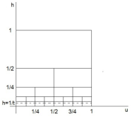
Figure 2: Square division in the proof of Proposition 4.1

An application of Boole’s inequality yields

$$\mathbb{P}\left\{\sup_{(u,v)\in A_{t}}\frac{a(t)(\nu(ut)-\nu(vt))}{(u-v)^{\alpha-\delta}}>x\right\}$$

$$\leq\sum_{j=1}^{\lceil\log_{2}t\rceil}\sum_{k=1}^{2^{j-1}}\mathbb{P}\left\{\frac{a(t)(\nu(tk2^{-j+1})-\nu(t((k-2)2^{-j+1})))}{2^{-j(\alpha-\delta)}}>x\right\}.$$

By distributional subadditivity (see formula (5.7) on p. 58 in [10]) of $(\nu(t))_{t\geq 0}$ (for $k\geq 3$) and by monotonicity of $(\nu(t))_{t\geq 0}$ (for $k=1,2$)

$$\mathbb{P}\left\{\frac{a(t)(\nu(tk2^{-j+1})-\nu(t((k-2)2^{-j+1})))}{2^{-j(\alpha-\delta)}}>x\right\}\leq\mathbb{P}\{a(t)\nu(t2^{-j+2})>x2^{-j(\alpha-\delta)}\}$$

whence

$$\mathbb{P}\left\{\sup_{(u,v)\in A_{t}}\frac{a(t)(\nu(ut)-\nu(vt))}{(u-v)^{\alpha-\delta}}>x\right\}\leq\sum_{j=1}^{\lceil\log_{2}t\rceil}2^{j-1}\mathbb{P}\{a(t)\nu(t2^{-j+2})>x2^{-j(\alpha-\delta)}\}$$

$$=\sum_{j=1}^{\lceil\log_{2}t\rceil}2^{j-1}\mathbb{P}\{\exp(a(t2^{-j+2})\nu(t2^{-j+2}))>\exp(x2^{-j(\alpha-\delta)}a(t2^{-j+2})/a(t))\}$$

$$\leq\sum_{j=1}^{\lceil\log_{2}t\rceil}2^{j-1}\exp(-x2^{-j(\alpha-\delta)}a(t2^{-j+2})/a(t))\,\mathbb{E}\exp(a(t2^{-j+2})\nu(t2^{-j+2}))$$

$$\leq C\sum_{j=1}^{\lceil\log_{2}t\rceil}2^{j-1}\exp(-x2^{-j(\alpha-\delta)}a(t2^{-j+2})/a(t)),$$

where the penultimate line is a consequence of Markov’s inequality, and the boundedness of $\mathbb{E}\exp(a(t2^{-j+2})\nu(t2^{-j+2}))$ follows from Lemma 7.4. Applying Lemma 7.5 to the function $a$ we obtain

$$a(t2^{-j+2})/a(t)\geq c2^{(j-2)(\alpha-\delta/2)}$$

for some $c>0$, all $t>0$ large enough and all $j=2,\ldots,\lceil\log_{2}t\rceil$. Hence,

$$\limsup_{t\to\infty}\mathbb{P}\left\{\sup_{(u,v)\in A_{t}}\frac{a(t)(\nu(ut)-\nu(vt))}{(u-v)^{\alpha-\delta}}>x\right\}\leq C\bigg{(}\exp(-x2^{\delta-\alpha})+\sum_{j\geq 2}2^{j-1}\exp(-c_{1}x2^{\delta j/2})\bigg{)},$$

where $c_{1}:=c2^{\delta-2\alpha}>0$. The last series converges uniformly in $x\in[1,\infty)$. Sending $x\to\infty$ finishes the proof. ∎

Acknowledgments  A part of this work was done while A. Iksanov was visiting University of Münster in January–February 2016. He gratefully acknowledges hospitality and the financial support by DFG SFB 878 “Geometry, Groups and Actions”. The work of A. Marynych was supported by the Alexander von Humboldt Foundation.

References

- [1] Alsmeyer, G., Iksanov, A. and Marynych, A. (2016+). Functional limit theorems for the number of occupied boxes in the Bernoulli sieve. Submitted. Preprint available at http://arxiv.org/abs/1601.04274
- [2] Baeumer, B., Meerschaert, M. and Nane, E. (2009). Space-time duality for fractional diffusion. J. Appl. Probab. 46, 1100–1115.
- [3] Bertoin, J. (1999). Subordinators: Examples and applications. LNM 1717, P.Bernard (Ed.), 1–91. Berlin: Springer-Verlag.
- [4] Bertoin J. and Yor, M. (2005). Exponential functionals of Lévy processes. Probability Surveys. 2, 191–212.
- [5] Billingsley, P. (1999). Convergence of probability measures, 2nd edition. New York: John Wiley and Sons.
- [6] Bingham N. H., Goldie C. M., and Teugels, J. L. (1989). Regular variation. Cambridge: Cambridge University Press.
- [7] Doney, R. A. and O’Brien, G. L. (1991). Loud shot noise. Ann. Appl. Probab. 1, 88–103.
- [8] Erdös, P. and Rényi, A. (1959). On Cantor’s series with convergent . Ann. Univ. Sci. Budapest. Eötvös. Sect. Math. 2, 93–109.
- [9] Fristedt, B. (1979). Uniform local behavior of stable subordinators. Ann. Probab. 7, 1003–1013.
- [10] Gut, A. (2009). Stopped random walks. Limit theorems and applications, 2nd edition. New York: Springer.
- [11] Jung, P., Owada, T. and Samorodnitsky, G. (2016+). Functional central limit theorem for negatively dependent heavy-tailed stationary infinitely divisible processes generated by conservative flows. Preprint available at http://arxiv.org/abs/1504.00935
- [12] Hawkes, J. (1971). A lower Lipschitz condition for the stable subordinator. Z. Wahrscheinlichkeitstheorie Verw. Geb. 17, 23–32.
- [13] Homble, P. and McCormick, W. P. (1995). Weak limit results for the extremes of a class of shot noise processes. J. Appl. Probab. 32, 707–726.
- [14] Hsing, T. and Teugels, J. L. (1989). Extremal properties of shot noise processes. Adv. Appl. Probab. 21, 513–525.
- [15] Iksanov, A. (2013). Functional limit theorems for renewal shot noise processes with increasing response functions. Stoch. Proc. Appl. 123, 1987–2010.
- [16] Iksanov, A. (2013). On the number of empty boxes in the Bernoulli sieve I. Stochastics: An International Journal of Probability and Stochastic Processes. 85, 946–959.
- [17] Iksanov A., Kabluchko, Z. and Marynych, A. (2016+). Weak convergence of renewal shot noise processes in the case of slowly varying normalization. Submitted. Preprint available at http://arxiv.org/abs/1507.02526
- [18] Iksanov, A., Marynych, A. and Meiners, M. (2013). Limit theorems for renewal shot noise processes with decreasing response functions. Extended preprint version of [19] at http://arxiv.org/abs/arXiv:1212.1583v2.
- [19] Iksanov, A., Marynych, A. and Meiners, M. (2014). Limit theorems for renewal shot noise processes with eventually decreasing response functions. Stoch. Proc. Appl. 124, 2132–2170.
- [20] Iksanov, A., Marynych, A. and Meiners, M (2016). Asymptotics of random processes with immigration I: Scaling limits. Bernoulli, to appear.
- [21] Iksanov, A., Marynych, A. and Meiners, M (2016). Asymptotics of random processes with immigration II: Convergence to stationarity. Bernoulli, to appear.
- [22] Lamperti, J. (1972). Semi-stable Markov processes. Z. Wahrscheinlichkeitstheorie Verw. Geb. 22, 205–-225.
- [23] Lebedev, A. V. (2002). Extremes of subexponential shot noise. Math. Notes. 71, 206–210.
- [24] Magdziarz, M. and Schilling, R. L. (2015). Asymptotic properties of Brownian motion delayed by inverse subordinators. Proc. Amer. Math. Soc. 143, 4485–4501.
- [25] Magdziarz, M. and Weron, A. (2011). Ergodic properties of anomalous diffusion processes. Ann. Phys. 326, 2431–2443.
- [26] McCormick, W. P. (1997). Extremes for shot noise processes with heavy tailed amplitudes. J. Appl. Probab. 34, 643–656.
- [27] McCormick, W. P. and Seymour, L. (2001). Extreme values for a class of shot-noise processes. In Selected Proceedings of the Symposium on Inference for Stochastic Processes, 33–46, Institute of Mathematical Statistics Lecture Notes - Monograph Series.
- [28] Meerschaert, M., Benson, D., Scheffler, H.-P. and Baeumer, B (2002). Stochastic solution of space–time fractional diffusion equations. Phys. Rev. E. 63, 1103–1106.
- [29] Meerschaert, M., Nane, E. and Vellaisamy, P. (2009). Fractional Cauchy problems on bounded domains. Ann. Probab. 37, 979–1007.
- [30] Meerschaert, M. and Scheffler, H.-P. (2004). Limit theorems for continuous-time random walks with infinite mean waiting times. J. Appl. Probab. 41, 623–638.
- [31] Meerschaert, M. and Straka, P. (2013). Inverse stable subordinators. Math. Model. Nat. Phenom. 8, 1–16.
- [32] Nane, E. (2009). Laws of the iterated logarithm for a class of iterated processes. Stat. Prob. Letters 79, 1744–1751.
- [33] Owada, T. and Samorodnitsky, G. (2015). Functional central limit theorem for heavy tailed stationary infinitely divisible processes generated by conservative flows. Ann. Probab. 43, 240–285.
- [34] Pardo, J. C., Rivero, V. and van Schaik, K. (2013). On the density of exponential functionals of Lévy processes. Bernoulli. 19, 1938–1964.
- [35] Rivero, V. (2003). A law of iterated logarithm for increasing self-similar Markov processes. Stochastics and Stochastics Reports. 75, 443–-472.
- [36] Samko, St. G., Kilbas, A. A. and Marichev, O. I. (1993). Fractional integrals and derivatives: theory and applications. New York: Gordon and Breach.
- [37] Scalas, E. and Viles, N. (2014). A functional limit theorem for stochastic integrals driven by a time-changed symmetric -stable Lévy process. Stoch. Proc. Appl. 124, 385–410.
- [38] Stanislavsky, A., Weron, K. and Weron, A. (2008). Diffusion and relaxation controlled by tempered -stable processes. Phys. Rev. E. 78, 051106.
- [39] Whitt, W. (2002). Stochastic-process limits: an introduction to stochastic-process limits and their application to queues. New York: Springer-Verlag.