Lattice Boltzmann simulations of 3D crystal growth: Numerical schemes for a phase-field model with anti-trapping current

Abstract

A lattice-Boltzmann (LB) scheme, based on the Bhatnagar-Gross-Krook (BGK) collision rules is developed for a phase-field model of alloy solidification in order to simulate the growth of dendrites. The solidification of a binary alloy is considered, taking into account diffusive transport of heat and solute, as well as the anisotropy of the solid-liquid interfacial free energy. The anisotropic terms in the phase-field evolution equation, the phenomenological anti-trapping current (introduced in the solute evolution equation to avoid spurious solute trapping), and the variation of the solute diffusion coefficient between phases, make it necessary to modify the equilibrium distribution functions of the LB scheme with respect to the one used in the standard method for the solution of advection-diffusion equations. The effects of grid anisotropy are removed by using the lattices D3Q15 and D3Q19 instead of D3Q7. The method is validated by direct comparison of the simulation results with a numerical code that uses the finite-difference method. Simulations are also carried out for two different anisotropy functions in order to demonstrate the capability of the method to generate various crystal shapes.

1 Introduction

With its local collision rules and its easy numerical implementation, the Lattice Boltzmann Equation (LBE) [1, 2] is a very attractive method to simulate the dynamics of complex fluids. Indeed, over more than twenty years, the LBE was successfully applied to simulate various problems of fluid dynamics, including two-phase flows separated by an interface [3, 4]. Other applications, such as flow and transport in unsaturated porous media [5, 6, 7], hydrodynamics coupled with magnetism [8, 9], and even solidification processes [10] were also developed.

The phase-field method has become, in recent years, one of the most popular methods for simulations of crystal growth and microstructure evolution in materials [11, 12, 13]. In this approach, the geometry of domains and interfaces is described by one or several scalar functions, the phase fields, that take constant values within each domain and vary smoothly but rapidly through the interfaces. The evolution equations for the phase fields, which give the interface dynamics without the need for an explicit front-tracking algorithm, are nonlinear partial differential equations (PDEs) that can be obtained from the principles of out-of-equilibrium thermodynamics. Therefore, they also naturally incorporate thermodynamic boundary conditions at the interfaces, such as the Gibbs-Thomson condition. Moreover, it is straightforward to introduce interfacial anisotropy in phase-field models, which makes it possible to perform accurate simulations of dendritic growth.

In problems of crystal growth, fluid flow often plays a dominant role. Indeed, the transport of heat and components from or to the growing crystal creates density variations in the liquid that trigger natural convection. Fluid flow may also be induced by external fields (temperature gradients, magnetic stirring etc.). Therefore, a complete description of crystal growth requires the coupling of the growth model with a fluid flow solver. Several phase-field models for solidification that are coupled to the Navier-Stokes equations for fluid flow have been proposed in the literature ([14, 15, 16]). In most cases, direct numerical simulations of these equations with finite-difference or finite-element methods are employed to solve the coupled model (see for example [17, 18, 19, 20]).

Many works also exist in the literature that combine the lattice Boltzmann method with models of solidification or crystal growth [21, 22, 23, 24, 25, 26, 27, 28]. Nevertheless, in those papers, the LBE is often used to simulate the fluid flow only, whereas the model of phase change is simulated with another numerical method (e.g. finite difference). In some examples where the LBE is applied to simulate solidification in the presence of interfacial anisotropy, the model used to track the interface between the solid and the liquid is not based on the phase-field theory. For instance in [27], the Gibbs-Thomson condition at the interface is explicitly solved in the numerical procedure, which corresponds to a <<sharp interface>> method. In [10, 29, 23] the model is based on the <<enthalpy-porosity>> approach, an alternative model of solid/liquid phase transition for a pure substance [30, 31].

Here, we propose a lattice Boltzmann scheme for a phase-field model of binary alloy solidification [32] that takes into account diffusive transport of heat and solute, as well as the anisotropy of the solid-liquid interfacial free energy. For this phase-field model, the relationships with its equivalent <<sharp interface>> equations are well established. When the diffusion coefficient is not the same in the solid and the liquid, the corrections of the <<thin interface limit>> of the phase-field model require adding a phenomenological flux, the anti-trapping current [33, 34]. This model is chosen as a reference by many authors, or used as a basis by others (see [35, 13] for a pedagogical presentation and [36, 37, 38] for extensions).

For the development of our scheme, we start from existing LBE formulations for reaction-diffusion equations. Those are based on the same steps as the LBE for fluid flow: streaming and collision. In order to apply this formalism to the equations of the phase-field model, several modifications must be made. In particular, the presence of i) interfacial anisotropy and ii) the anti-trapping current require to choose appropriate equilibrium distribution functions, to be used in the collision step. The choice of these functions is dictated by analytical calculations (a Chapman-Enskog expansion of the LBE equation).

We perform various tests to validate our new scheme. First, we check the influence of the grid anisotropy on simulated crystal shapes. We find that for lattices with a sufficient number of streaming directions, this anisotropy is very low (a fraction of a percent). Next, we directly compare simulations of dendritic growth in a pure substance and in an isothermal binary alloy to respective simulations performed with a finite-difference scheme used in the literature [39, 33]. We find excellent agreement. Finally, we also demonstrate that, in agreement with previous studies [40], our scheme can produce various dendritic shapes (with different growth directions of the main branches) if the anisotropy function is changed.

As a result, we achieve a full implementation of the phase-field model in the LBE framework. This has some interesting properties, such as easy implementation and straightforward parallelization. In addition, the same concepts involved in fluid dynamics (definitions of lattices, collision, displacement, bounce-back …) can be applied, such that a seamless and easy integration with a LBE solver for fluid flow becomes possible.

The rest of this paper is organized as follows. The phase-field model for solidification of a dilute binary mixture is presented in Section 2. The lattice Boltzmann scheme and details about the algorithm implementation are described in Section 3. Section 4 presents results of validations and simulations. Finally, the conclusions are presented in Section 5.

2 Phase-field model

We consider a phase-field model for the solidification of a single crystal from a quiescent melt; the fluid is considered at rest and the density is assumed to be a constant, equal in the liquid and the solid. Fluid flow is not taken into account in the model. The details of the model development can be found in [32]; here, we will only summarize the most important points. The sharp-interface problem, formulated in terms of the local alloy composition $c$ and temperature $T$ is:

$$\partial_{t}c =D\boldsymbol{\nabla}^{2}c \mbox{{\rm(liquid)}},\qquad$$ (1a)

$$\partial_{t}T =\kappa\boldsymbol{\nabla}^{2}T \mbox{{\rm(liquid and solid)}},\qquad$$ (1b)

$$c_{l}(1-k)V_{n} =-D\partial_{n}c_{l} \mbox{{\rm(interface)}},\qquad$$ (1c)

$$LV_{n} =C_{p}\kappa(\partial_{n}T|_{s}-\partial_{n}T|_{l}) \mbox{{\rm(interface)}},\qquad$$ (1d)

$$T_{i} =T_{m}+mc_{l}-\Gamma{\cal K}-V_{n}/\mu_{k} \mbox{{\rm(interface)}}.\qquad$$ (1e)

The first two of these equations describe diffusive transport of heat and solute according to Fick’s and Fourier’s laws, with $D$ the solute diffusion coefficient, and $\kappa$ the thermal diffusivity. The latter, as well as the specific heat $C_{p}$, is assumed to be the same in the two phases (symmetric model). In contrast, solute transport is assumed to take place in the liquid only (one-sided model). The next two equations express mass and heat conservation at the moving boundary (Stefan conditions), with $V_{n}$ the normal velocity of the interface, $k=c_{s}/c_{l}$ the partition coefficient that relates the compositions of solid and liquid in contact with each other at the interface, $L$ the latent heat of melting, and the symbol $\partial_{n}$ denoting the spatial derivative in the direction normal to the interface. Indeed, in the phase diagram for a dilute binary mixture, the crystal has a lower solute concentration than the liquid, so that solute has to be redistributed upon interface motion. The latent heat of melting is also set free upon crystallization and generates heat fluxes away from the interface. The last equation is the Gibbs-Thomson boundary condition, which relates the interface temperature to the composition of the adjacent liquid $c_{l}$, the interface curvature ${\cal K}$ and the interface velocity. Here, $T_{m}$ is the melting temperature of the pure solvent, $m$ the slope of the liquidus line in the phase diagram, $\Gamma=\gamma T_{m}/L$ the Gibbs-Thomson constant, with $\gamma$ being the solid-liquid surface free energy, and $\mu_{k}$ is the interface mobility. Note that, for simplicity, we have written down here the isotropic version of the Gibbs-Thomson condition.

For the following, it is useful to introduce scaled fields:

$$\theta =\frac{T-T_{m}-mc_{\infty}}{L/C_{p}},$$ (2)

$$U =\frac{c-c_{\infty}}{(1-k)c_{\infty}},$$ (3)

where $c_{\infty}$ is the initial composition of the melt. In terms of these fields, the equations become:

$$\partial_{t}U =D\boldsymbol{\nabla}^{2}U,$$ (4a)

$$\partial_{t}\theta =\kappa\boldsymbol{\nabla}^{2}\theta,$$ (4b)

$${}[1+(1-k)U_{i}]V_{n} =-D\partial_{n}U,$$ (4c)

$$V_{n} =\kappa(\partial_{n}\theta|_{s}-\partial_{n}\theta|_{l}),$$ (4d)

$$\theta_{i}+Mc_{\infty}U_{i} =-d_{0}{\cal K}-\beta V_{n}.$$ (4e)

Here, quantities evaluated at the interface have a subscript $i$, $M=-m(1-k)C_{p}/L$ is the scaled magnitude of the liquidus slope,

$$d_{0}=\frac{\Gamma C_{p}}{L}=\frac{\gamma T_{m}C_{p}}{L^{2}}$$ (5)

is the capillary length, with $\gamma$ the solid-liquid surface energy, and

$$\beta=\frac{C_{p}}{L\mu_{k}}$$ (6)

the interface kinetic coefficient.

In the phase-field formulation of this problem [32], the interface position is implicitly described as a level set of a phase-field function $\phi$. The phase field takes the value $\phi=1$ in the solid and $\phi=-1$ in the liquid. Furthermore, the field $U$ is expressed in terms of $\phi$ and $c$ as

$$U=\frac{\frac{c/c_{\infty}}{\frac{1}{2}[1+k-(1-k)\phi]}-1}{1-k}.$$ (7)

This definition extends $U$ to the entire domain (solid, liquid, and interfaces); in the liquid, it is identical to Eq. (3). At equilibrium, $U$ is constant across the diffuse interface. In fact, $U$ is a scaled diffusion potential (see [41] for details).

The model consists of three coupled partial differential equations for the three fields $\phi$, $\theta$, and $U$ which read:

$$\tau(\mathbf{n})\frac{\partial\phi}{\partial t} =W_{0}^{2}\boldsymbol{\nabla}\cdot(a_{s}^{2}(\mathbf{n})\boldsymbol{\nabla}\phi)+W_{0}^{2}\boldsymbol{\nabla}\cdot\boldsymbol{\mathcal{N}}+(\phi-\phi^{3})-\lambda\left(Mc_{\infty}U+\theta\right)(1-\phi^{2})^{2},$$ (8a)

$$\left(\frac{1+k}{2}-\frac{1-k}{2}\phi\right)\frac{\partial U}{\partial t} =\boldsymbol{\nabla}\cdot\left(Dq(\phi)\boldsymbol{\nabla}U-\mathbf{j}_{\mbox{at}}\right)+\left[1+\left(1-k\right)U\right]\frac{1}{2}\frac{\partial\phi}{\partial t},$$ (8b)

$$\frac{\partial\theta}{\partial t} =\kappa\boldsymbol{\nabla}^{2}\theta+\frac{1}{2}\frac{\partial\phi}{\partial t}.$$ (8c)

Here, $W_{0}$ denotes the characteristic width of the diffuse interfaces, and the coefficient $\lambda$ describes the strength of the coupling between the phase field and the transport fields. The relaxation time of the phase field is noted $\tau(\mathbf{n})$ and depends on the unit normal vector at the interface $\mathbf{n}=-\boldsymbol{\nabla}\phi/\bigl{|}\boldsymbol{\nabla}\phi\bigr{|}$. We choose $\tau(\mathbf{n})=\tau_{0}a_{s}^{2}(\mathbf{n})$, where $\tau_{0}$ is a constant and $a_{s}(\mathbf{n})$ is an anisotropy function. For most of the following, we use the standard choice:

$$a_{s}(\mathbf{n})=1-3\varepsilon_{s}+4\varepsilon_{s}\sum_{\alpha=x,y,z}n_{\alpha}^{4},$$ (9)

which describes a cubic anisotropy of strength $\varepsilon_{s}$ in three dimensions, with $n_{\alpha}$ ($\alpha=x,\,y,\,z$) being the Cartesian $\alpha$-component of $\mathbf{n}$. The presence of the anisotropy on the right-hand side of Eq. (8a) arises from an anisotropic surface free energy; the function $\boldsymbol{\mathcal{N}}\equiv\boldsymbol{\mathcal{N}}(\mathbf{x},\,t)$ is a vector defined by:

$$\boldsymbol{\mathcal{N}}(\mathbf{x},\,t)=\bigl{|}\boldsymbol{\nabla}\phi\bigr{|}^{2}a_{s}(\mathbf{n})\left(\frac{\partial a_{s}(\mathbf{n})}{\partial(\partial_{x}\phi)},\,\frac{\partial a_{s}(\mathbf{n})}{\partial(\partial_{y}\phi)},\,\frac{\partial a_{s}(\mathbf{n})}{\partial(\partial_{z}\phi)}\right)^{T}.$$ (10)

Expressions of the derivatives $\partial a_{s}(\mathbf{n})/\partial(\partial_{\alpha}\phi)$ will be specified in subsection 3.4.

In Eq. (8b), $q(\phi)=(1-\phi)/2$ is a function that interpolates the solute diffusivity between $D$ in the liquid and 0 in the solid. $\mathbf{j}_{\mbox{at}}$ is the phenomenological anti-trapping current introduced in [33] in order to counterbalance spurious solute trapping without introducing other thin-interface effects (see also [42, 34]). It is defined by:

$$\mathbf{j}_{\mbox{at}}(\mathbf{x},\,t)=-\frac{1}{2\sqrt{2}}W_{0}\left[1+\left(1-k\right)U\right]\times\frac{\partial\phi}{\partial t}\frac{\boldsymbol{\nabla}\phi}{\bigl{|}\boldsymbol{\nabla}\phi\bigr{|}}.$$ (11)

This current is proportional to the velocity ($\partial_{t}\phi)$ and the thickness $W_{0}$ of the interface, is normal to the interface, and pointing from solid to liquid ($-\boldsymbol{\nabla}\phi/\bigl{|}\boldsymbol{\nabla}\phi\bigr{|}$). While the other components of the model can be derived variationally from an appropriate free-energy functional, the anti-trapping current was introduced for phenomenological reasons and justified by carrying out matched asymptotic expansions, which demonstrated that the model with the anti-trapping current is indeed equivalent to the sharp-interface problem [34]. Let us mention that, recently, an alternative justification for this current has been proposed [43, 44]. In any case, the matched asymptotic expansions provide a relation between phase-field and sharp-interface parameters given by:

$$d_{0} =a_{1}\frac{W_{0}}{\lambda},$$ (12a)

$$\beta =a_{1}\left(\frac{\tau_{0}}{W_{0}\lambda}-a_{2}\frac{W_{0}}{D}\left[\frac{D}{\kappa}+Mc_{\infty}[1+(1-k)U]\right]\right),$$ (12b)

with $a_{1}$ and $a_{2}$ being numbers of order unity. For the model used here, $a_{1}=5\sqrt{2}/8$, and $a_{2}\approx 0.6267$. These relations make it possible to choose phase-field parameters for prescribed values of the capillary length (surface energy) and the interface mobility (interface kinetic coefficient). Note that the interface width $W_{0}$ is a parameter that can be freely chosen in this formulation; the asymptotic analysis remains valid as long as $W_{0}$ remains much smaller than any length scale present in the sharp-interface solution of the considered problem (for example, a dendrite tip radius in the case of dendritic growth).

The model presented above can be seen as a combination of the earlier phase-field formulations for the symmetric model [39] and the one-sided model [33, 34], which have been widely used. More detailed derivations and discussions of the model equations can be found in these references.

3 Lattice Boltzmann schemes

Eqs. (8a)–(8c) with the additional relationships (9)–(11) represent the mathematical model considered in this work. In this section, the numerical method based on the LBE will be described for each equation of the model. The LBE is an evolution equation in time and space of a discrete function, the distribution function of particles, which is defined over a lattice. The choice of the lattice determines the number of streaming directions of the distribution function. Once the LBE is defined, the algorithm can be summarized in three main operations applied on this distribution function: the first one is a moving step on the lattice; the second one is a collision step that relaxes the distribution function towards an equilibrium, the equilibrium distribution function, with a relaxation rate. Finally, the last stage is to update the physical variable, such as the dimensionless temperature, or the phase field, by computing its moment of order zero.

In this section we detail each stage of the method: the LBE will be presented and the equilibrium distribution functions will be defined as well as the relaxation rates. Next, various lattices will be introduced and some details will be given about the algorithm implementation. For a pedagogical presentation, we start the description with the LB scheme for the heat equation, because it is the simplest equation of the model for which the standard LB method can be applied. For the two other ones, the collision step and the equilibrium distribution function have to be modified. Derivation of equilibrium distribution functions, which couples the physical variables and the lattice-dependent quantities, is the most delicate part of the numerical scheme. The derivations of such functions necessitate to carry out asymptotic calculations (Chapman-Enskog expansion) that can be found in A and B for Eqs. (8a) and (8b) respectively.

3.1 Heat equation: standard lattice Boltzmann scheme

The heat equation (8c) is a diffusion equation with a source term. For that equation, the standard LB-BGK equation is applied:

$$f_{i}(\mathbf{x}+\mathbf{e}_{i}\delta x,\,t+\delta t)=f_{i}(\mathbf{x},\,t)-\frac{1}{\eta_{\theta}}\left[f_{i}(\mathbf{x},\,t)-f_{i}^{(0)}(\mathbf{x},\,t)\right]+w_{i}Q_{\theta}(\mathbf{x},\,t)\delta t,$$ (13a)

where $f_{i}(\mathbf{x},\,t)$ is a distribution function which can be regarded as an intermediate function introduced to calculate the dimensionless temperature $\theta$. This latter is calculated by:

$$\theta(\mathbf{x},\,t)=\sum_{i=0}^{N_{pop}}f_{i}(\mathbf{x},\,t),$$ (13b)

where the index $i$ identifies the moving directions on a lattice: $i=0,\,...,\,N_{pop}$ where $N_{pop}$ is the total number of directions. $\mathbf{e}_{i}$ is the vector of displacement on that lattice and $w_{i}$ are weights. The quantities $N_{pop}$, $\mathbf{e}_{i}$ and $w_{i}$ are lattice-dependent and will be defined in subsection 3.4. The time-step is noted $\delta t$ and the space-step is noted $\delta x$ by assuming $\delta x=\delta y=\delta z$. In Eq. (13a), the equilibrium distribution function $f_{i}^{(0)}$ and the source term $Q_{\theta}$ are given by:

$$f_{i}^{(0)}(\mathbf{x},\,t) =w_{i}\theta(\mathbf{x},\,t),$$ (13c)

$$Q_{\theta}(\mathbf{x},\,t) =\frac{1}{2}\frac{\partial\phi}{\partial t}.$$ (13d)

In such a method, the thermal diffusivity $\kappa$ is related to the relaxation time of collision $\eta_{\theta}$ by:

$$\kappa=e^{2}\left(\eta_{\theta}-\frac{1}{2}\right)\frac{\delta x^{2}}{\delta t},$$ (13e)

where $e^{2}$ is an additional lattice-dependent coefficient which arises from the second-order moment of $f_{i}^{(0)}$. The values of $e^{2}$ will be given in subsection 3.4 for several lattices. The index $\theta$ in $Q_{\theta}$ and $\eta_{\theta}$ indicates that both quantities are relative to the heat equation. In a more general case, the thermal diffusivity $\kappa$ is a function depending on space and time. In that case, the relationship (13e) must be inverted and the relaxation parameter has to be updated at each time step.

The principle of the LB scheme is the following. Once the dimensionless temperature $\theta$ is known, the equilibrium distribution function $f_{i}^{(0)}$ is computed by using Eq. (13c). The collision stage (right-hand side of Eq. (13a)) is next calculated and yields an intermediate distribution function that will be streamed in each direction (left-hand side of Eq. (13a)). Finally after updating the boundary conditions, the new temperature is calculated by using Eq. (13b) and the algorithm is iterated in time. Notice that the scheme is fully explicit: all terms in the right-hand side of Eq. (13a) are defined at time $t$. Also note that the source term $Q_{\theta}$ involves the time derivative of the phase field. In practice, the heat equation must be solved after solving the phase-field equation. At the first time-step, the derivative can be evaluated thanks to the knowledge of the phase field and the initial condition. Finally, this scheme can be easily extended to simulate the Advection-Diffusion Equation (ADE) by modifying the equilibrium distribution function such as $f_{i}^{(0)\,ADE}=w_{i}\theta\left[1+e^{-2}\mathbf{e}_{i}\cdot\mathbf{v}\delta t/\delta x\right]$ where $\mathbf{v}$ is the advective velocity. Moments of zeroth-, first- and second-order of $f_{i}^{(0)\,ADE}$ are respectively $\theta$, $\mathbf{v}\theta\delta t/\delta x$ and $e^{2}\theta\overline{\overline{\mathbf{I}}}$ where $\overline{\overline{\mathbf{I}}}$ is the identity tensor of rank 2.

3.2 Phase-field equation: modification of collision stage

The phase-field equation looks like an ADE with an additional factor $\tau(\mathbf{n})$ in front of the time derivative. In order to handle this factor and the divergence term $\boldsymbol{\nabla}\cdot\boldsymbol{\mathcal{N}}$, the standard LB scheme is modified in the following form:

$$a_{s}^{2}(\mathbf{n})g_{i}(\mathbf{x}+\mathbf{e}_{i}\delta x,\,t+\delta t)=g_{i}(\mathbf{x},\,t)-(1-a_{s}^{2}(\mathbf{n}))g_{i}(\mathbf{x}+\mathbf{e}_{i}\delta x,\,t)-\frac{1}{\eta_{\phi}(\mathbf{x},\,t)}\left[g_{i}(\mathbf{x},\,t)-g_{i}^{(0)}(\mathbf{x},\,t)\right]+w_{i}Q_{\phi}(\mathbf{x},\,t)\frac{\delta t}{\tau_{0}},$$ (14a)

with the equilibrium distribution function $g_{i}^{(0)}(\mathbf{x},\,t)$ defined by:

$$g_{i}^{(0)}(\mathbf{x},\,t)=w_{i}\left(\phi(\mathbf{x},\,t)-\frac{1}{e^{2}}\mathbf{e}_{i}\cdot\boldsymbol{\mathcal{N}}(\mathbf{x},\,t)\frac{\delta t}{\delta x}\frac{W_{0}^{2}}{\tau_{0}}\right).$$ (14b)

In Eq. (14a), $g_{i}$ is the distribution function for the phase field $\phi$ calculated by $\phi=\sum_{i=0}^{N_{pop}}g_{i}$ after the streaming step. Moments of zeroth-, first- and second-order of the equilibrium distribution function $g_{i}^{(0)}$ are respectively $\sum_{i=0}^{N_{pop}}g_{i}^{(0)}=\phi$, $\sum_{i=0}^{N_{pop}}g_{i}^{(0)}\mathbf{e}_{i}=-\boldsymbol{\mathcal{N}}\delta tW_{0}^{2}/(\tau_{0}\delta x)$, and $\sum_{i=0}^{N_{pop}}g_{i}^{(0)}\mathbf{e}_{i}\mathbf{e}_{i}=e^{2}\phi\overline{\overline{\mathbf{I}}}$ where $\overline{\overline{\mathbf{I}}}$ is still the identity tensor of rank 2 (see A). The scalar function $Q_{\phi}(\mathbf{x},\,t)$ is the source term of the phase-field equation (8a) defined by:

$$Q_{\phi}(\mathbf{x},\,t) =\left[\phi-\lambda(Mc_{\infty}U+\theta)(1-\phi^{2})\right](1-\phi^{2}).$$ (14c)

In Eq. (8a) the coefficient $a_{s}^{2}(\mathbf{n})$ plays a similar role as a <<diffusion>> coefficient depending on position and time (through $\mathbf{n}$ that depends on $\phi$). The relaxation time $\eta_{\phi}(\mathbf{x},\,t)$ is a function of position and time and must be updated at each time step by the relationship:

$$\eta_{\phi}(\mathbf{x},\,t)=\frac{1}{e^{2}}a_{s}^{2}(\mathbf{n})\frac{W_{0}^{2}}{\tau_{0}}\frac{\delta t}{\delta x^{2}}+\frac{1}{2}.$$ (14d)

The lattice Boltzmann scheme for the phase-field equation differs from the standard LB method for ADE on two points. The first difference is the presence in Eq. (14a) of (i) a factor $a_{s}^{2}(\mathbf{n})$ in front of $g_{i}(\mathbf{x}+\mathbf{e}_{i}\delta x,\,t+\delta t)$ in the left-hand side of Eq. (14a) and (ii) an additional term $(1-a_{s}^{2}(\mathbf{n}))g_{i}(\mathbf{x}+\mathbf{e}_{i}\delta x,\,t)$ in the right-hand side. The latter term is non-local in space, i.e., it is involved in the collision step at time $t$ and needs the knowledge of $g_{i}$ at the neighboring nodes $\mathbf{x}+\mathbf{e}_{i}\delta x$. Those two terms appear to handle the factor $a_{s}^{2}(\mathbf{n})$ in front of the time derivative $\partial\phi/\partial t$ in Eq. (8a). We can see it by carrying out the Taylor expansions of $g_{i}(\mathbf{x}+\mathbf{e}_{i}\delta x,\,t+\delta t)$ and $g_{i}(\mathbf{x}+\mathbf{e}_{i}\delta x,\,t)$ (see A). The method is inspired from [45].

The second difference with the LB algorithm for ADE, is the definition of the equilibrium distribution function $g_{i}^{(0)}$ (Eq. (14b)). The absence of phase field $\phi(\mathbf{x},\,t)$ in the divergence term (8a), explains its presence in the first term inside the brackets (14b). Moreover, note the sign change in front of the scalar product, corresponding to the sign change of advective term in ADE to $+\boldsymbol{\nabla}\cdot\boldsymbol{\mathcal{N}}$ for the phase-field equation. Finally, the presence of factor $W_{0}^{2}/\tau_{0}$ in Eqs. (14b) and (14d) can be understood by dividing each term of Eq. (8a) by $\tau_{0}$ and by comparing this equation with the equation for moments of $g_{i}^{(0)}$ (see Eq. (25) in A) derived from the asymptotic expansions of Eq. (14a).

3.3 Supersaturation equation: modification of the equilibrium distribution function

In the usual lattice BGK scheme for ADE, the diffusion coefficient $Dq(\phi)$ would be related to the relaxation time $\eta_{U}$ with the relationship $Dq(\phi)=e^{2}(\eta_{U}-1/2)\delta x^{2}/\delta t$. However, in Eq. (8b), the interpolation function $q(\phi)$ cancels the diffusion coefficient inside the solid part. By following the standard method, the relaxation time would be equal to $1/2$ in the solid part which would lead to the occurrence of instabilities of the algorithm. Moreover, another source of instabilities appeared by applying the non-local method of the previous subsection for factor $((1+k)-(1-k)\phi)/2\equiv\zeta(\phi)$ in front of the time derivative. In practice, instabilities of algorithm occurred for several values of the partition coefficient $k$. In order to overcome these difficulties, the supersaturation equation was reformulated in the following way:

$$\frac{\partial U}{\partial t}=\boldsymbol{\nabla}\cdot\left[D\boldsymbol{\nabla}\left(\frac{q(\phi)}{\zeta(\phi)}U(\mathbf{x},\,t)\right)\right]-\boldsymbol{\nabla}\cdot\mathbf{J}_{\mbox{tot}}(\mathbf{x},\,t)+S(\mathbf{x},\,t)+\frac{Q_{U}(\mathbf{x},\,t)}{\zeta(\phi)},$$ (15a)

with :

$$\mathbf{J}_{\mbox{tot}}(\mathbf{x},\,t) =D\left[\boldsymbol{\nabla}\left(\frac{q(\phi)}{\zeta(\phi)}\right)+q(\phi)\mathbf{F}(\phi)\right]U+\frac{\mathbf{j}_{\mbox{at}}}{\zeta(\phi)},$$ (15b)

$$S(\mathbf{x},\,t) =U\boldsymbol{\nabla}\cdot(Dq(\phi)\mathbf{F}(\phi))+\mathbf{j}_{\mbox{at}}\cdot\mathbf{F}(\phi),$$ (15c)

$$Q_{U}(\mathbf{x},\,t) =\left[1+\left(1-k\right)U\right]\frac{1}{2}\frac{\partial\phi}{\partial t},$$ (15d)

where $\mathbf{F}(\phi)=\boldsymbol{\nabla}(1/\zeta(\phi))$. The relationships (15a)–(15d) arise from successive applications of $\boldsymbol{\nabla}(ab)=a\boldsymbol{\nabla}b+b\boldsymbol{\nabla}a$ and $\boldsymbol{\nabla}\cdot(a\mathbf{c})=a\boldsymbol{\nabla}\cdot\mathbf{c}+\mathbf{c}\cdot\boldsymbol{\nabla}a$ where $a$ and $b$ are two scalar functions and $\mathbf{c}$ is a vectorial function. Note that the inverse of $\zeta(\phi)$ can be calculated because this function never vanishes for $k>0$. Indeed $\zeta(\phi)=k$ if $\phi=+1$, $\zeta(\phi)=1$ if $\phi=-1$ and varies linearly between those two values for $-1<\phi<+1$.

The lattice Boltzmann method for simulating the supersaturation equation is:

$$h_{i}(\mathbf{x}+\mathbf{e}_{i}\delta x,\,t+\delta t)=h_{i}(\mathbf{x},\,t)-\frac{1}{\eta_{U}}\left[h_{i}(\mathbf{x},\,t)-h_{i}^{(0)}(\mathbf{x},\,t)\right]+w_{i}\left[S(\mathbf{x},\,t)+\frac{Q_{U}(\mathbf{x},\,t)}{\zeta(\phi)}\right]\delta t,$$ (16a)

with an equilibrium distribution function $h_{i}^{(0)}(\mathbf{x},\,t)$ defined as (see B):

$$h_{i}^{(0)}(\mathbf{x},\,t)=A_{i}U(\mathbf{x},\,t)+B_{i}\left(\frac{q(\phi)}{\zeta(\phi)}U(\mathbf{x},\,t)+\frac{1}{e^{2}}\mathbf{e}_{i}\cdot\mathbf{J}_{\mbox{tot}}(\mathbf{x},\,t)\frac{\delta t}{\delta x}\right).$$ (16b)

In Eq. (16a), $h_{i}$ is the distribution function for the supersaturation: $U=\sum_{i=0}^{N_{pop}}h_{i}$. The equilibrium distribution function $h_{i}^{(0)}(\mathbf{x},\,t)$ was derived such as its moments of zeroth-, first- and second-order are respectively $\sum_{i=0}^{N_{pop}}h_{i}^{(0)}=U$, $\sum_{i=0}^{N_{pop}}h_{i}^{(0)}\mathbf{e}_{i}=\mathbf{J}_{\mbox{tot}}\delta t/\delta x$, and $\sum_{i=0}^{N_{pop}}h_{i}^{(0)}\mathbf{e}_{i}\mathbf{e}_{i}=e^{2}(q(\phi)/\zeta(\phi))U\overline{\overline{\mathbf{I}}}$ (see B). The values of weights $A_{i}$ and $B_{i}$ are indicated in subsection 3.4 for several lattices. The relaxation time $\eta_{U}$ is calculated before the time iterations by:

$$\eta_{U}=\frac{1}{e^{2}}\frac{\delta t}{\delta x^{2}}D+\frac{1}{2}.$$ (16c)

With this formulation, the interpolation function $q(\phi)$ and the relaxation coefficient $\eta_{U}$ are decoupled. Once $\delta x$ and $\delta t$ are fixed, $\eta_{U}$ keeps the same constant value in the whole computational domain, even in the solid part. The function $q(\phi)$ appears inside three terms: the laplacian term, the total flux $\mathbf{J}_{\mbox{tot}}$ and the source term $S$. The second advantage of this formulation is that the standard collision scheme can be kept to handle the factor $\zeta(\phi)$ in the LB scheme. Nevertheless, additional gradients of $\zeta(\phi)$ and $q(\phi)$ have to be evaluated with this formulation.

3.4 Definitions of lattices and algorithm implementation

Definitions of Lattices

In order to study the effects of grid anisotropy, which arise from discretization of the phase-field equation [39, 46, 47], three 3D lattices were used in this work: D3Q7, D3Q15 and D3Q19 (Fig. 1). The total number of moving directions for each lattice is respectively $N_{pop}=6,$ $14$ and $18$. The displacement vectors are defined in Tab. 1 for all lattices. The D3Q7-lattice is defined by seven vectors, for D3Q15 eight directions are added to the previous ones, corresponding to the eight diagonals of the cube, and for D3Q19 we consider 12 additional directions. For each one of them, the LB schemes described in the previous subsections remain identical. The values of weights $w_{i}$, $A_{i}$ , $B_{i}$ and $e^{2}$ are indicated in Tab. 2. For completeness, we introduce the 2D lattices D2Q5 and D2Q9 for 2D simulations of validation. The vectors of displacement are defined in Tab. 3 and the values of weights in Tab. 4.

(a) D3Q7	(b) D3Q15	(c) D3Q19

Figure 1: 3D lattices of LB scheme.

Table 1: Definition of moving vectors $\mathbf{e}_{i}$ for 3D lattices

Definition of $\mathbf{e}_{i}$ for D3Q7

$\mathbf{e}_{0}=\left(\begin{array}[]{c}0\\ 0\\ 0\end{array}\right)$ $\mathbf{e}_{1}=\left(\begin{array}[]{c}1\\ 0\\ 0\end{array}\right)$ $\mathbf{e}_{2}=\left(\begin{array}[]{c}0\\ 1\\ 0\end{array}\right)$ $\mathbf{e}_{3}=\left(\begin{array}[]{c}-1\\ 0\\ 0\end{array}\right)$ $\mathbf{e}_{4}=\left(\begin{array}[]{c}0\\ -1\\ 0\end{array}\right)$ $\mathbf{e}_{5}=\left(\begin{array}[]{c}0\\ 0\\ 1\end{array}\right)$ $\mathbf{e}_{6}=\left(\begin{array}[]{c}0\\ 0\\ -1\end{array}\right)$

Additional $\mathbf{e}_{i}$ vectors for D3Q15

$\mathbf{e}_{7}=\left(\begin{array}[]{c}1\\ 1\\ 1\end{array}\right)$ $\mathbf{e}_{8}=\left(\begin{array}[]{c}-1\\ 1\\ 1\end{array}\right)$ $\mathbf{e}_{9}=\left(\begin{array}[]{c}-1\\ -1\\ 1\end{array}\right)$ $\mathbf{e}_{10}=\left(\begin{array}[]{c}1\\ -1\\ 1\end{array}\right)$ $\mathbf{e}_{11}=\left(\begin{array}[]{c}1\\ 1\\ -1\end{array}\right)$ $\mathbf{e}_{12}=\left(\begin{array}[]{c}-1\\ 1\\ -1\end{array}\right)$ $\mathbf{e}_{13}=\left(\begin{array}[]{c}-1\\ -1\\ -1\end{array}\right)$ $\mathbf{e}_{14}=\left(\begin{array}[]{c}1\\ -1\\ -1\end{array}\right)$

Additional $\mathbf{e}_{i}$ vectors for D3Q19

$\mathbf{e}_{7}=\left(\begin{array}[]{c}1\\ 1\\ 0\end{array}\right)$ $\mathbf{e}_{8}=\left(\begin{array}[]{c}-1\\ 1\\ 0\end{array}\right)$ $\mathbf{e}_{9}=\left(\begin{array}[]{c}1\\ -1\\ 0\end{array}\right)$ $\mathbf{e}_{10}=\left(\begin{array}[]{c}-1\\ -1\\ 0\end{array}\right)$ $\mathbf{e}_{11}=\left(\begin{array}[]{c}1\\ 0\\ 1\end{array}\right)$ $\mathbf{e}_{12}=\left(\begin{array}[]{c}-1\\ 0\\ 1\end{array}\right)$ $\mathbf{e}_{13}=\left(\begin{array}[]{c}1\\ 0\\ -1\end{array}\right)$ $\mathbf{e}_{14}=\left(\begin{array}[]{c}-1\\ 0\\ -1\end{array}\right)$ $\mathbf{e}_{15}=\left(\begin{array}[]{c}0\\ 1\\ 1\end{array}\right)$ $\mathbf{e}_{16}=\left(\begin{array}[]{c}0\\ -1\\ 1\end{array}\right)$ $\mathbf{e}_{17}=\left(\begin{array}[]{c}0\\ 1\\ -1\end{array}\right)$ $\mathbf{e}_{18}=\left(\begin{array}[]{c}0\\ -1\\ -1\end{array}\right)$

Table 2: Values of $w_{i}$, $A_{i}$, $B_{i}$ and $e^{2}$ for 3D lattices ($\times$: irrelevant)

Lattices	Weights for of $\phi$- and $\theta$-Eq.	Weights for $U$-Eq.
Lattice $N_{pop}$ $e^{2}$ D3Q7 $6$ $1/4$ D3Q15 $14$ $1/3$ D3Q19 $18$ $1/3$	$w_{0}$ $w_{1,...,6}$ $w_{7,...,14}$ $w_{7,...,18}$ $1/4$ $1/8$ $\times$ $\times$ $2/9$ $1/9$ $1/72$ $\times$ $1/3$ $1/18$ $\times$ $1/36$	$A_{0}$ $A_{1,...,6}$ $A_{7,...,14}$ $A_{7,...,18}$ $B_{0}$ $B_{1,...,6}$ $B_{7,...,14}$ $B_{7,...,18}$ $1$ $0$ $\times$ $\times$ $-3/4$ $1/8$ $\times$ $\times$ $1$ $0$ $0$ $\times$ $-7/9$ $1/9$ $1/72$ $\times$ $1$ $0$ $\times$ $0$ $-2/3$ $1/18$ $\times$ $1/36$

(a) D2Q5		(b) D2Q9

Figure 2: 2D Lattices of LB scheme.

Table 3: Definition of moving vectors $\mathbf{e}_{i}$ for 2D lattices

Definition of vectors for D2Q5

$\mathbf{e}_{0}=\left(\begin{array}[]{c}0\\ 0\end{array}\right)$ $\mathbf{e}_{1}=\left(\begin{array}[]{c}1\\ 0\end{array}\right)$ $\mathbf{e}_{2}=\left(\begin{array}[]{c}0\\ 1\end{array}\right)$ $\mathbf{e}_{3}=\left(\begin{array}[]{c}-1\\ 0\end{array}\right)$ $\mathbf{e}_{4}=\left(\begin{array}[]{c}0\\ -1\end{array}\right)$

Additional vectors for D2Q9

$\mathbf{e}_{5}=\left(\begin{array}[]{c}1\\ 1\end{array}\right)$ $\mathbf{e}_{6}=\left(\begin{array}[]{c}-1\\ 1\end{array}\right)$ $\mathbf{e}_{7}=\left(\begin{array}[]{c}-1\\ -1\end{array}\right)$ $\mathbf{e}_{8}=\left(\begin{array}[]{c}1\\ -1\end{array}\right)$

Table 4: Values of $w_{i}$, $A_{i}$, $B_{i}$ and $e^{2}$ for 2D lattices ($\times$: irrelevant)

Lattices	Weights for $\phi$- and $\theta$-Eq.	Weights for $U$-Eq.
Lattice $N_{pop}$ $e^{2}$ D2Q5 $4$ $1/3$ D2Q9 $8$ $1/3$	$w_{0}$ $w_{1,...,4}$ $w_{5,...,8}$ $1/3$ $1/6$ $\times$ $4/9$ $1/9$ $1/36$	$A_{0}$ $A_{1,...,4}$ $A_{5,...,8}$ $B_{0}$ $B_{1,...,4}$ $B_{5,...,8}$ $1$ $0$ $\times$ $-2/3$ $1/6$ $\times$ $1$ $0$ $0$ $-5/9$ $1/9$ $1/36$

Algorithm implementation

The algorithm is sequential: after solving the phase-field equation, the phase-field $\phi$ is used to calculate the time evolution of the supersaturation $U$ and the temperature $\theta$. For each equation, the standard stages of lattice Boltzmann method are applied. Each LB equation (13a), (14a) and (16a), is separated into one collision step followed by one streaming step of each distribution function $f_{i}$, $g_{i}$ and $h_{i}$. The factors $a_{s}^{2}(\mathbf{n})$ and $\zeta(\phi)$ are treated explicitly. The collision stage for the phase-field equation writes:

$$g_{i}^{\star}(\mathbf{x},\,t) =\frac{1}{a_{s}^{2}(\mathbf{n})}\biggl{\{}g_{i}(\mathbf{x},\,t)-(1-a_{s}^{2}(\mathbf{n}))g_{i}(\mathbf{x}+\mathbf{e}_{i}\delta x,\,t)-\frac{1}{\eta_{\phi}(\mathbf{x},\,t)}\left[g_{i}(\mathbf{x},\,t)-g_{i}^{(0)}(\mathbf{x},\,t)\right]+w_{i}Q(\mathbf{x},\,t)\frac{\delta t}{\tau_{0}}\biggr{\}},$$ (17a)

where the symbol $\star$ means the distribution function after the collision. The standard collision ($a_{s}^{2}(\mathbf{n})=1$) is considered on boundary nodes. The moving step writes:

$$g_{i}(\mathbf{x}+\mathbf{e}_{i}\delta x,\,t+\delta t)=g_{i}^{\star}(\mathbf{x},\,t).$$ (17b)

For each LB scheme, the update of boundary conditions is carried out by the <<bounce back>> rule. For instance in the phase-field scheme $g_{i}(\mathbf{x},\,t)=g_{i^{\prime}}(\mathbf{x},\,t)$ where $i^{\prime}$ is the opposite direction of $i$. The computation of gradient $\boldsymbol{\nabla}\phi$ needed for the normal vector $\mathbf{n}$ is carried out by a centered finite difference method. Finally, the computation of vector $\boldsymbol{\mathcal{N}}(\mathbf{x},\,t)$ for each time step needs the calculation of derivatives $\partial a_{s}(\mathbf{n})/\partial(\partial_{\alpha}\phi)$ for $\alpha=x,\,y,\,z$, which write:

$$\frac{\partial a_{s}(\mathbf{n})}{\partial(\partial_{\alpha}\phi)} =-\frac{16\varepsilon_{s}}{\bigl{|}\boldsymbol{\nabla}\phi\bigr{|}^{6}}\times(\partial_{\alpha}\phi)\Bigl{[}(\partial_{\beta}\phi)^{4}-(\partial_{\alpha}\phi)^{2}(\partial_{\beta}\phi)^{2}-(\partial_{\alpha}\phi)^{2}(\partial_{\gamma}\phi)^{2}+(\partial_{\gamma}\phi)^{4}\Bigr{]}.$$ (18)

In this equation, the first component of $\boldsymbol{\mathcal{N}}$ is obtained for $\alpha\equiv x$, $\beta\equiv y$ and $\gamma\equiv z$. The second one is obtained for $\alpha\equiv y$, $\beta\equiv x$ and $\gamma\equiv x$ and finally the third one for $\alpha\equiv z$, $\beta\equiv x$ and $\gamma\equiv y$. The gradient terms involved in Eq. (15b) and (15c) are calculated with a centered finite difference method. The partial derivative in time $\partial\phi/\partial t$ in Eqs. (8b), (8c) and (11) is discretized by an Euler scheme.

4 Validations and simulations

For simulations, the computational domain is cubic and zero fluxes are imposed on all boundaries for each equation. For the phase-field equation, a nucleus is initialized as a diffuse sphere: $\phi(\mathbf{x},\,0)=\tanh\left[(R_{s}-d_{s})/\sqrt{l_{s}}\right]$ where $R_{s}$ is the radius, $d_{s}=\sqrt{(x-x_{s})^{2}+(y-y_{s})^{2}+(z-z_{s})^{2}}$ and $\mathbf{x}_{s}=(x_{s},\,y_{s},\,z_{s})^{T}$ is the position of its center. With this initial condition, $\phi=+1$ inside the sphere and $\phi=-1$ outside. The coefficient $l_{s}$ decreases or increases the slope of $\phi$-profile between its minimal and maximal values. In this work $l_{s}=2W_{0}$ as indicated in [48]. For equations of supersaturation and temperature, the initial conditions are constant on the whole domain: $U(\mathbf{x},\,0)=U_{0}$ and $\theta(\mathbf{x},\,0)=\theta_{0}$.

4.1 Crystal growth of pure substance: 3D grid effects and validation with a benchmark

We consider the basic problem of solidification of a pure substance. For this problem, the phase-field model is composed of two equations [39], the first one for the phase-field Eq. (8a) by setting $M=0$ and the second one for the dimensionless temperature Eq. (8c). The lattice Boltzmann schemes of subsections 3.1 and 3.2 are checked with a finite difference scheme. Following [46], the discrete laplacian of phase-field equation is obtained by using respectively 6 (FD6) and 18 (FD18) nearest neighboring nodes. Simulations are first carried out for an isotropic case, i.e. with $\varepsilon_{s}=0$, for studying the lattice effects. Next, the anisotropic term ($\varepsilon_{s}\neq 0$) will be considered for comparison of the numerical implementation of LB schemes with another code.

Isotropic case: $\varepsilon_{s}=0$

For this simulation, the mesh is composed of $301^{3}$ nodes, the space-step is equal to $\delta x=0.01$ and the time-step is $\delta t=1.5\times 10^{-5}$. The interface thickness is equal to $W_{0}=0.01$, the scale factor in time is $\tau_{0}=10^{-4}$. Finally $\varepsilon_{s}=0.05$, $\lambda=10$ and $\kappa=0.7$. The sphere radius is equal to $R_{s}=8$ lattice unit (l.u.). The iso-values $\phi=0$ of the phase field are presented in Fig. 3 at $t=10^{4}\delta t$ for three lattices D3Q7, D3Q15 and D3Q19. In this figure, the initial condition and the results obtained with FD6 and FD18 are plotted for comparison. Slices are made for two different planes: the normal vector of the first one is $(0,\,0,\,1)$ (Fig. 3a), and the normal vector of the second one is $(1,\,0,\,-1)$ (Fig. 3b). In each figure, the shapes of solutions obtained by LB-D3Q15, LB-D3Q19 and FD18 are circles that overlap, contrary to those obtained by LB-D3Q7 and FD6. The profiles collected along the directions $\mathbf{n}_{1}=(1,\,0,\,0)$ and $\mathbf{n}_{2}=(1,\,1,\,0)$ (Fig. 4), present more accurately the effects of <<grid anisotropy>> (or mesh anisotropy) of those two latter methods. The grid anisotropy can be quantified by introducing a coefficient $\mathcal{A}_{g}$ [47]: $\mathcal{A}_{g}=\left|(R_{100}-R_{110})/(R_{100}+R_{110})\right|\times 100$, where $R_{100}$ is the radius measured along the $x$-axis in the $\mathbf{n}_{1}$-direction and $R_{110}$ is the radius measured at 45° between of the $x$-axis in the $\mathbf{n}_{2}$-direction. The value of $\mathcal{A}_{g}$ is lower than one percent ($0.073$%) for D3Q15 and is equal to $0.116$% for D3Q19. For D3Q7, the grid anisotropy is equal to $3.095$%. For the finite difference schemes, $\mathcal{A}_{g}$ is equal to $4.365$% for FD6 and $0.575$% for FD18. Results obtained with the D3Q15 lattice are slightly more accurate because it is well-suited when the solidification occurs as a sphere. Indeed, that lattice takes into account the diagonals of the cube and allows the displacement of distribution function $f_{i}$ in the diagonal directions, contrary to the D3Q19 (see Fig. 1b,c).

(a) Plane of normal vector $(0,\,0,\,1)^{T}$	(b) Plane of normal vector $(1,\,0,\,-1)^{T}$
	(view in $xy$-plane)

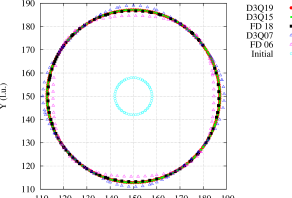
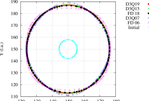
Figure 3: Iso-values $\phi=0$ of phase field for LB and FD schemes at $t=10^{4}\delta t$. Results from LB-D3Q15, LB-D3Q19 and FD18 form circles which match, contrary to those arising from LB-D3Q7. The initial condition is given for comparison.

(a) Direction $(1,\,0,\,0)$		(b) Direction $(1,\,1,\,0)$

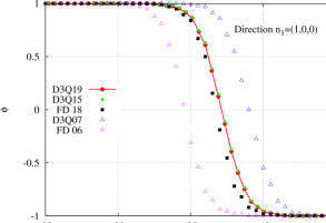
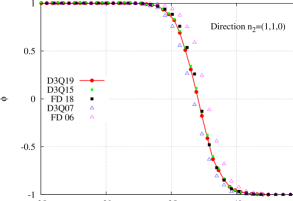
Figure 4: Phase-field profiles for directions $\mathbf{n}_{1}$ (a) and $\mathbf{n}_{2}$ (b). Profiles calculated by LB-D3Q15, LB-D3Q19 and FD18 fit for both directions unlike those obtained by LB-D3Q7 and FD6.

Anisotropic case: $\varepsilon_{s}\neq 0$

Now the validation of the numerical implementation is carried out by considering an anisotropic case. We use for the comparison a 2D numerical code based on a Finite Difference (FD) method for the phase-field equation and a Monte-Carlo (MC) algorithm for the temperature [49]. In what follows, the results of this method will be labeled by FDMC. For the LB schemes, we use the lattices D2Q9 for Eq. (8a) and D2Q5 for Eq. (8c). The results will be labeled by LBE.

The domain is a square discretized with meshes of size $\delta x$. The initial seed is a diffuse circle of radius $R_{s}=10\delta x$ which is set at the origin of the computational domain. The problem is symmetrical with respect to the $x$-axis and $y$-axis. In this test, we compare the shape of the dendrite given by $\phi=0$ and the evolution of the tip velocity. The interface thickness $W_{0}$ and the characteristic time $\tau_{0}$ are set to $W_{0}=\tau_{0}=1$. The space step is chosen such as $\delta x/W_{0}=0.4$ [39], the time step is $\delta t=0.008$ and the lengths of the system depend on the undercooling $\Delta=-\theta_{0}$. A smaller undercooling necessitates a bigger mesh because of the larger diffusive length. The time to reach the stationary velocity is also more important. We present below the results for two undercoolings: $\Delta_{1}=0.30$ and $\Delta_{2}=0.55$. For the first one, we use a mesh of $1000^{2}$ nodes and for the second one, a mesh of $500^{2}$ nodes.

In the phase-field theory, the capillary length $d_{0}$ and the kinetic coefficient $\beta$ are given by [39]: $d_{0}=a_{1}W_{0}/\lambda$ and $\beta=a_{1}(\tau_{0}/\lambda W_{0}-a_{2}W_{0}/\kappa)$ where $a_{1}=0.8839$ and $a_{2}=0.6267$. In this benchmark, we choose the parameter $\lambda$ such as $\beta=0$, i.e. $\lambda^{\star}=\kappa\tau_{0}/a_{2}W_{0}^{2}$. By considering $W_{0}=1$ and $\tau_{0}=1$, the coefficient $\lambda^{\star}$ is equal to $\lambda^{\star}=\kappa/a_{2}=1.59566\kappa$. For a thermal diffusivity equals to $\kappa=4$, we obtain $\lambda^{\star}=6.3826$ and $d_{0}=0.1385$. Finally the anisotropic strength is $\varepsilon_{s}=0.05$.

In the comparisons, the velocity $V_{p}$ is dimensionless by using the factor $d_{0}/\kappa$ ($V_{p}=\tilde{V}_{p}d_{0}/\kappa$), the position $x$ is also dimensionless by using the space-step ($x=\tilde{x}/\delta x$) and the time $T$ is the time $t$ divided by $\tau_{0}$ ($T=t/\tau_{0}$). Fig. 5 presents the results of comparisons for $\Delta_{1}=0.30$ and $\Delta_{2}=0.55$. For each numerical method, the tip velocity fits well (Fig. 5a) as well as the dendrite shape (Fig. 5b). On this figure, the full dendrite is reconstructed by symmetry for the LBE method. For the FDMC method, only the first quadrant is presented. For $\Delta_{2}=0.55$, we remark a slight difference between both curves during the initial transient that precedes steady-state growth (in a time range from $t=0$ to $t=100$), but the steady-state velocities converge toward values that are close to each other. Indeed, at $t=300$, $V_{p}^{LBE}=0.01735$ and $V_{p}^{FDMC}=0.01667$, representing a relative error of 4%. For this benchmark, let us emphasize that the value of $V_{p}$ reported in [39] (Table II) is $V_{p}=0.0174$ and $V_{p}^{GF}=0.0170$ (where the $GF$ notation stands for the Green’s Function method, which is a sharp-interface method considered as a reference), representing a relative error of 0.3% between LBE and the first value, and 2% between LBE and the second value.

(a)		(b)

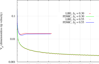
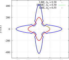
Figure 5: (a) Dimensionless tip velocity $V_{p}$ as a function of time for $\Delta_{1}=0.30$ and $\Delta_{2}=0.55$. (b) Superposition of $\phi=0$ for FDMC (green line) and LBE (red dots) at $t=1.3\times 10^{5}\delta t$ for $\Delta_{1}$. For $\Delta_{2}$, the shape $\phi=0$ is given for comparison at $t=4\times 10^{4}\delta t$. Parameters are $\kappa=4$, $\lambda^{\star}=6.3826$, $d_{0}=0.1385$ and $\varepsilon_{s}=0.05$.

4.2 Validation of supersaturation LB scheme

The LB scheme for the supersaturation equation defines a new equilibrium distribution function (Eq. (16b)) and necessitates to calculate additional gradients in Eqs. (15b) and (15c). In order to check this method, an additional benchmark is carried out by combining Eq. (8a) coupled with Eq. (8b) including the anti-trapping current $\mathbf{j}_{\mbox{at}}$ (Eq. (11)). For this benchmark we consider an isothermal solidification, i.e. $\theta=0$, and the parameters are $U_{0}=-0.55$, $D=2$, $k=0.15$, $W_{0}=1$, $\tau_{0}=1$, $\varepsilon_{s}=0.03$, $\lambda^{\star}=3.2$, $d_{0}=0.2762$, $R_{s}=10$ l.u., $Mc_{\infty}=1$, $\delta x=0.4$, and $\delta t=0.02$.The LB results are compared with a finite-difference code that is comparable to the one used in [33]. The tip velocity is presented in Fig. 6; the good agreement validates the lattice Boltzmann scheme with anti-trapping current.

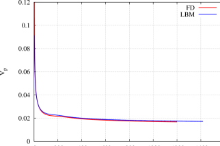
Figure 6: Dimensionless tip velocity $V_{p}$ of an isothermal dilute alloy dendrite as a function of time for $U_{0}=-0.55$.

4.3 Simulations of non standard dendrites

The anisotropy function (Eq. (9)) defines an interfacial excess free energy which favors a preferential growth in the direction [100]. Those directions correspond to the directions of the main axes $x$, $y$ and $z$. Other preferential directions of growth can be simulated by modifying this function on the basis of spherical and cubic harmonics [40]. In the present section, we compare the classical function (9) with another one defined by [50]:

$$a_{s}(\mathbf{n})=1+\varepsilon_{s}\left(\sum_{\alpha=x,y,z}n_{\alpha}^{4}-\frac{3}{5}\right)+\delta\left(3\sum_{\alpha=x,y,z}n_{\alpha}^{4}+66n_{x}^{2}n_{y}^{2}n_{z}^{2}-\frac{17}{7}\right).$$ (19)

The second term in the right-hand side of Eq. (19) is the cubic harmonic $K_{41}$ and the last term corresponds to the cubic harmonic $K_{61}$. In the LB method, the $a_{s}(\mathbf{n})$ function and its derivatives are involved in the function $\boldsymbol{\mathcal{N}}(\mathbf{x},\,t)$ inside the equilibrium distribution function Eq. (14b). For both simulations the kinetic coefficient is chosen such as $\tau(\mathbf{n})=\tau_{0}a_{s}^{2}(\mathbf{n})$, the mesh is composed of $351^{3}$ nodes, $\delta x=0.01$, $\delta t=1.5\times 10^{-5}$, $W_{0}=0.0125$, $\tau_{0}=1.5625\times 10^{-4}$, $\lambda=10$, $\kappa=1$ and $\Delta=0.25$. The first simulation is carried out by using Eq. (9) and $\varepsilon_{s}=0.05$, and the second one with Eq. (19), $\varepsilon_{s}=0$ and $\delta=-0.02$. The system is initialized with a sphere of radius $R_{s}=8$ l.u. at the origin of the domain. The problem is symmetrical with respect to the planes $xy$, $xz$ and $yz$. A comparison of the shapes $\phi=0$ is presented in Fig. 7 for a same orientation of the landmark. The method is thus able to simulate easily different crystal shapes by modifying the function $\boldsymbol{\mathcal{N}}(\mathbf{x},\,t)$.

(a)		(b)

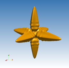
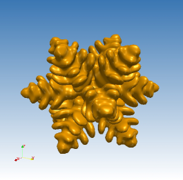
Figure 7: (a) [100] preferential growth at $t=3\times 10^{4}\delta t$ with $\varepsilon_{s}=0.05$. (b) [110] preferential growth at $t=1.4\times 10^{5}\delta t$ with $\varepsilon_{s}=0$ and $\delta=-0.02$.

5 Conclusion

We have presented a lattice Boltzmann method to simulate a crystal growth model for a binary mixture with anti-trapping current. The method requires a modification of the equilibrium distribution functions and needs to consider a non-local collision for the phase-field equation to take into account respectively the term responsible for the anisotropic growth and the kinetic coefficient in front of the time derivative. The use of lattices D3Q15 and D3Q19 for the phase-field equation improves the accuracy of the solutions by removing the undesired effect of grid anisotropy. The method was validated by comparison with other codes based on the finite-difference method. Finally, the method is able to simulate other anisotropic functions with minor modifications of the code in order to generate preferential directions of dendritic growth other than [100].

The numerical method presented in this paper for the solidification of alloys under diffusive heat and solute transport uses the same concepts as those involved in the simulation of fluid flows: the lattices (D2Q9, D3Q15, D3Q19) are identical and the same stages of collision, displacement and bounce back are applied. This will make it easier to directly couple the phase-field model and the Navier-Stokes equations in order to study, for example, the density change effect during the solidification process or the effect of convective fluid flow on crystal growth. The advective terms that have to be added in each equation of the phase-field model, can be taken into account by modifying the equilibrium distribution functions of each equation according to standard procedures. Studies including such couplings will be the subject of future works.

Appendix A Chapman-Enskog expansions for phase-field equation

We present in this appendix the Chapman-Enskog expansions for the phase-field equation. In the first part, the continuous equation for the moments of the equilibrium distribution function $g_{i}^{(0)}$ is established. In the second part, we focus on the derivation of a specific form of the equilibrium distribution function $g_{i}^{(0)}$. For more concision, dependencies in $\mathbf{x}$ and $t$ are canceled in functions $g_{i}$, $\eta_{\phi}$ and $Q$. We also assume the dependency of $a_{s}^{2}$ with $\mathbf{n}$.

Taylor and asymptotic expansions

Taylor expansion at second-order in space and first-order in time of Eq. (14a) yields:

$$a_{s}^{2}\left[g_{i}+\delta x\mathbf{e}_{i}\cdot\boldsymbol{\nabla}g_{i}+\frac{\delta x^{2}}{2}\mathbf{e}_{i}\mathbf{e}_{i}:\boldsymbol{\nabla}\boldsymbol{\nabla}g_{i}+\delta t\partial_{t}g_{i}\right] =g_{i}+(a_{s}^{2}-1)\left[g_{i}+\delta x\mathbf{e}_{i}\cdot\boldsymbol{\nabla}g_{i}+\frac{\delta x^{2}}{2}\mathbf{e}_{i}\mathbf{e}_{i}:\boldsymbol{\nabla}\boldsymbol{\nabla}g_{i}\right]$$

$$\qquad\qquad-\frac{1}{\eta_{\phi}}\left[g_{i}-g_{i}^{(0)}\right]+w_{i}Q_{\phi}\frac{\delta t}{\tau_{0}}$$ (20)

After simplification, the factor $a_{s}^{2}$ appears only in front of the time derivative $\partial_{t}g_{i}$:

$$a_{s}^{2}\delta t\partial_{t}g_{i}+\delta x\mathbf{e}_{i}\cdot\boldsymbol{\nabla}g_{i}+ \frac{\delta x^{2}}{2}\mathbf{e}_{i}\mathbf{e}_{i}:\boldsymbol{\nabla}\boldsymbol{\nabla}g_{i}=-\frac{1}{\eta_{\phi}}\left[g_{i}-g_{i}^{(0)}\right]+w_{i}Q_{\phi}\frac{\delta t}{\tau_{0}}.$$ (21)

From now on all steps are standard (see [1, 45]). Space and time are rescaled by introducing a small parameter $\epsilon=\delta x/L$ where $L$ is the characteristic length of the system. One scale in space $\mathbf{x}_{1}=\epsilon\mathbf{x}$ is considered and two time-scales $t_{1}=\epsilon t$ and $t_{2}=\epsilon^{2}t$ which are representative of convection and diffusion, respectively. With these notations, the partial derivatives write: $\boldsymbol{\nabla}=\epsilon\boldsymbol{\nabla}_{1}$ and $\partial_{t}=\epsilon\partial_{t_{1}}+\epsilon^{2}\partial_{t_{2}}$. The function $g_{i}$ is expanded in power of $\epsilon$ around $g_{i}^{(0)}$: $g_{i}\simeq g_{i}^{(0)}+\epsilon g_{i}^{(1)}.$ The moment of 0th-order of the distribution function $g_{i}$ is the phase field $\phi$: $\sum_{i}g_{i}=\phi$, which must be invariant during the collision step. That means $\sum_{i}g_{i}^{(0)}=\phi$ and involves $\sum_{i}g_{i}^{(1)}=0$. After substituting those relationships in (21), all terms in $\epsilon$- and those in $\epsilon^{2}$-order are combined into two distinct equations. For the first one, the moment of zeroth-order (sum over $i$) yields:

$$a_{s}^{2}\partial_{t_{1}}(\sum_{i}g_{i}^{(0)})+\frac{\delta x}{\delta t}\boldsymbol{\nabla}_{1}\cdot(\sum_{i}g_{i}^{(0)}\mathbf{e}_{i})=0,$$ (22)

and the moment of first-order (multiplying by $\mathbf{e}_{i}$ and summing over $i$) yields:

$$\sum_{i}g_{i}^{(1)}\mathbf{e}_{i}\simeq-\eta_{\phi}\delta x\boldsymbol{\nabla}_{1}\cdot(\sum_{i}g_{i}^{(0)}\mathbf{e}_{i}\mathbf{e}_{i}).$$ (23)

In (23), the term $\delta t\partial_{t_{1}}\sum_{i}g_{i}^{(0)}\mathbf{e}_{i}$ was assumed negligible, assumption that can be removed by modifying the collision stage (see [51] for BGK-collision, [52] for TRT-collision and [53, 54] for MRT-collision). For Eq. in $\epsilon^{2}$-order, by using (23), the calculation of zeroth-order moment yields:

$$a_{s}^{2}\partial_{t_{2}}(\sum_{i}g_{i}^{(0)})=\boldsymbol{\nabla}_{1}\cdot\left[\left(\eta_{\phi}-\frac{1}{2}\right)\frac{\delta x^{2}}{\delta t}\boldsymbol{\nabla}_{1}\cdot(\sum_{i}g_{i}^{(0)}\mathbf{e}_{i}\mathbf{e}_{i})\right].$$ (24)

Finally, by combining all terms $\epsilon^{0}\times\sum_{i}w_{i}Q_{\phi}/\tau_{0}$ + $\epsilon^{1}\times$Eq. (22) + $\epsilon^{2}\times$Eq. (24), the continuous partial differential equation for the three first moments of $g_{i}^{(0)}$ is:

$$a_{s}^{2}\partial_{t}(\sum_{i}g_{i}^{(0)}) =\boldsymbol{\nabla}\cdot\left[\left(\eta_{\phi}-\frac{1}{2}\right)\frac{\delta x^{2}}{\delta t}\boldsymbol{\nabla}\cdot(\sum_{i}g_{i}^{(0)}\mathbf{e}_{i}\mathbf{e}_{i})\right]-\frac{\delta x}{\delta t}\boldsymbol{\nabla}\cdot(\sum_{i}g_{i}^{(0)}\mathbf{e}_{i})+\sum_{i}w_{i}\frac{Q_{\phi}}{\tau_{0}}.$$ (25)

Equilibrium distribution function $g_{i}^{(0)}$

Comparison of Eqs. (25) and (8a) that is rewritten as:

$$a_{s}^{2}\frac{\partial\phi}{\partial t}=\frac{W_{0}^{2}}{\tau_{0}}\boldsymbol{\nabla}\cdot(a_{s}^{2}(\mathbf{n})\boldsymbol{\nabla}\phi)+\frac{W_{0}^{2}}{\tau_{0}}\boldsymbol{\nabla}\cdot\boldsymbol{\mathcal{N}}+\frac{Q_{\phi}}{\tau_{0}},$$ (26)

indicates that $g_{i}^{(0)}$ must be defined such that its moments of 0th-, 1rst- and 2nd-order have to be equal to $\sum_{i}g_{i}^{(0)}=\phi$, $\sum_{i}g_{i}^{(0)}\mathbf{e}_{i}=-\boldsymbol{\mathcal{N}}W_{0}^{2}\delta t/(\tau_{0}\delta x)$ and $\sum_{i}g_{i}^{(0)}\mathbf{e}_{i}\mathbf{e}_{i}=e^{2}\phi\overline{\overline{\mathbf{I}}}$ where $\overline{\overline{\mathbf{I}}}$ is the identity tensor of rank 2. The equilibrium distribution function $g_{i}^{(0)}$ is chosen as:

$$g_{i}^{(0)}=w_{i}\phi+w^{\prime}_{i}\mathbf{e}_{i}\cdot\boldsymbol{\mathcal{N}}\frac{\delta t}{\delta x}\frac{W_{0}^{2}}{\tau_{0}},$$ (27)

where we look for the coefficients $w_{i}$ and $w^{\prime}_{i}$. Values of weights and coefficient $e^{2}$ are detailed here for D3Q7 lattice defined in section 3. The generalization for D3Q15 and D3Q19 lattices is straightforward. Moment of 0th-order yields $\sum_{i}w_{i}\phi=\phi$ (the second term of the right-hand side vanishes) and its moment of first-order yields:

$$\sum_{i}w_{i}\phi\mathbf{e}_{i}+\sum_{i}w^{\prime}_{i}\left(\mathbf{e}_{i}\cdot\boldsymbol{\mathcal{N}}\frac{\delta t}{\delta x}\frac{W_{0}^{2}}{\tau_{0}}\right)\mathbf{e}_{i}=-\boldsymbol{\mathcal{N}}\frac{\delta t}{\delta x}\frac{W_{0}^{2}}{\tau_{0}},$$ (28)

where the first sum of the left-hand side vanishes. One obtains $w_{1}=w_{3}$, $w_{2}=w_{4}$ and $w_{5}=w_{6}$. One solution is to set $w_{0}=1/4$ and $w_{i=1,\,...,\,6}=1/8$. Regarding the weights $w^{\prime}_{k}$, the following relationships are obtained by identifying the components of each side of equality (28): $(w^{\prime}_{1}+w^{\prime}_{3})\mathcal{N}_{x}=-\mathcal{N}_{x}$, $(w^{\prime}_{2}+w^{\prime}_{4})\mathcal{N}_{y}=-\mathcal{N}_{y}$, $(w^{\prime}_{5}+w^{\prime}_{6})\mathcal{N}_{z}=-\mathcal{N}_{z}$. We deduce that $w^{\prime}_{i=1,\,...,\,6}=-1/2$. Calculation of second-order moment of Eq. (27) yields (by using values of weights $w_{i}$): $\sum_{i}g_{i}^{(0)}\mathbf{e}_{i}\mathbf{e}_{i}=\sum_{i}w_{i}\phi\mathbf{e}_{i}\mathbf{e}_{i}=(1/4)\phi\overline{\overline{\mathbf{I}}}.$ We set $e^{2}=1/4$ and $w^{\prime}_{i}=w_{i}/e^{2}$, we obtain $g_{i}^{(0)}=w_{i}\left(\phi-e^{-2}\mathbf{e}_{i}\cdot\boldsymbol{\mathcal{N}}\delta tW_{0}^{2}/(\tau_{0}\delta x)\right)$. Finally Eq. (8a) is derived by identifying $a_{s}^{2}W_{0}^{2}/\tau_{0}$ to $e^{2}(\zeta_{\phi}-1/2)\delta x^{2}/\delta t$.

Appendix B Equilibrium distribution function for the supersaturation equation

Following the same procedure as detailed in A, the partial differential equation for the moments of $h_{i}^{(0)}$ is obtained:

$$\partial_{t}(\sum_{i}h_{i}^{(0)}) =\boldsymbol{\nabla}\cdot\left[\left(\eta_{U}-\frac{1}{2}\right)\frac{\delta x^{2}}{\delta t}\boldsymbol{\nabla}\cdot(\sum_{i}h_{i}^{(0)}\mathbf{e}_{i}\mathbf{e}_{i})\right]-\frac{\delta x}{\delta t}\boldsymbol{\nabla}\cdot(\sum_{i}h_{i}^{(0)}\mathbf{e}_{i})+\sum_{i}w_{i}\left[S+\frac{Q_{U}}{\zeta}\right].$$ (29)

Comparison with Eq. (15a) indicates that $h_{i}^{(0)}$ must be defined such as $\sum_{i}h_{i}^{(0)}=U$, $\sum_{i}h_{i}^{(0)}\mathbf{e}_{i}=\mathbf{J}_{\mbox{tot}}\delta t/\delta x$ and $\sum_{i}h_{i}^{(0)}\mathbf{e}_{i}\mathbf{e}_{i}=e^{2}(q(\phi)/\zeta(\phi))U\overline{\overline{\mathbf{I}}}$. The equilibrium distribution function $h_{i}^{(0)}$ is set as follows:

$$h_{i}^{(0)}=A_{i}U+B_{i}\frac{q(\phi)}{\zeta(\phi)}U+C_{i}\mathbf{e}_{i}\cdot\mathbf{J}_{\mbox{tot}}\frac{\delta t}{\delta x},$$ (30)

where coefficients $A_{i}$, $B_{i}$ and $C_{i}$ have to be determined. Moment of 0th-order yields the first constraint $\sum_{i}A_{i}+B_{i}Dq(\phi)/\zeta(\phi)=1$ and the moment of 1rst-order yields the second one:

$$\sum_{i}\left(A_{i}+B_{i}\frac{q(\phi)}{\zeta(\phi)}\right)U\mathbf{e}_{i}+\sum_{i}\left(C_{i}\mathbf{e}_{i}\cdot\mathbf{J}_{\mbox{tot}}\frac{\delta t}{\delta x}\right)\mathbf{e}_{i} =\mathbf{J}_{\mbox{tot}}\frac{\delta t}{\delta x}.$$ (31)

One solution satisfying both equalities is: $A_{0}=1$, $A_{1,...,6}=0$, $B_{0}=-3/4$, $B_{1,...,6}=1/8$ and $C_{1,...,6}=1/2$. Using values of $A_{i}$ and $B_{i}$ for calculation of the 2nd-order moment, we check that: $\sum_{i}h_{i}^{(0)}\mathbf{e}_{i}\mathbf{e}_{i}=(1/4)(q(\phi)/\zeta(\phi))U\overline{\overline{\mathbf{I}}}$. We set $e^{2}=1/4$ and $C_{i}/B_{i}=1/e^{2}$. The expected supersaturation Eq. (8b) is obtained by identifying $D=e^{2}(\eta_{U}-1/2)(\delta x^{2}/\delta t)$.

References

- Chen and Doolen [1998] S. Chen, G. Doolen, Lattice Boltzmann Method for fluid flows, Annual Reviews of Fluid Mechanics 30 (1998) pp. 329–364.
- Guo and Shu [2013] Z. Guo, C. Shu, Lattice Boltzmann Method and its Applications in Engineering, vol. 3 of Advances in Computational Fluid Dynamics, World Scientific Publishing Co. Pte. Ltd., 2013.
- Lee [2009] T. Lee, Effects of incompressibility on the elimination of parasitic currents in the lattice Boltzmann equation method for binary fluids, Computers and Mathematics with Applications 58 (2009) pp. 987–994, doi:10.1016/j.camwa.2009.02.017.
- Lee and Liu [2010] T. Lee, L. Liu, Lattice Boltzmann simulations of micron-scale drop impact on dry surfaces, Journal of Computational Physics 229 (2010) 8045–8063, doi:10.1016/j.jcp.2010.07.007.
- Ginzburg [2005] I. Ginzburg, Equilibrium-type and link-type lattice Boltzmann models for generic advection and anisotropic-dispersion equation, Advances in Water Resources 28 (2005) pp. 1171–1195, doi:10.1016/j.advwatres.2005.03.004.
- Ginzburg [2008] I. Ginzburg, Consistent lattice Boltzmann schemes for the Brinkman model of porous flow and infinite Chapman-Enskog expansion, Physical Review E 77 (066704) (2008) 1–12.
- Genty and Pot [2013] A. Genty, V. Pot, Numerical Simulation of 3D Liquid-Gas Distribution in Porous Media by a Two-Phase TRT Lattice Boltzmann Method, Transport in Porous Media 96 (2013) pp. 271–294.
- Dellar [2002] P. Dellar, Lattice Kinetic Schemes for Magnetohydrodynamics, Journal of Computational Physics 179 (2002) pp. 95–126, doi:10.1006/jcph.2002.7044.
- Pattison et al. [2008] M. Pattison, K. Premnath, N. Morley, M. Abdou, Progress in lattice Boltzmann methods for magnetohydrodynamic flows relevant to fusion applications, Fusion Engineering and Design 83 (2008) pp. 557–572.
- Jiaung et al. [2001] W.-S. Jiaung, J.-R. Ho, C.-P. Kuo, Lattice Boltzmann method for the heat conduction problem with phase change, Numerical Heat Transfer 39 (2001) pp. 167–187.
- Boettinger et al. [2002] W. J. Boettinger, J. A. Warren, C. Beckermann, A. Karma, Phase-Field Simulation of Solidification, Annual Review of Materials Research 32 (2002) pp. 163–194, doi:10.1146/annurev.matsci.32.101901.155803.
- Singer-Loginova and Singer [2008] I. Singer-Loginova, H. M. Singer, The phase field technique for modeling multiphase materials, Reports on Progress in Physics 71 (2008) 106501, doi:http://dx.doi.org/10.1088/0034-4885/71/10/106501.
- Provatas and Elder [2010] N. Provatas, K. Elder, Phase-Field Methods in Materials Science and Engineering, Wiley-VCH, 2010.
- Beckermann et al. [1999] C. Beckermann, H.-J. Diepers, I. Steinbach, A. Karma, X. Tong, Modeling Melt Convection in Phase-Field Simulations of Solidification, Journal of Computational Physics 154 (1999) pp. 468–496, doi:10.1006/jcph.1999.6323.
- Anderson et al. [2000] D. M. Anderson, G. B. McFadden, A. A. Wheeler, A phase-field model of solidification with convection, Physica D 135 (2000) pp. 175–194.
- Conti [2001] M. Conti, Density change effects on crystal growth from the melt, Physical Review E 64 (051601) (2001) pp. 1–9.
- Tönhardt and Amberg [2000] R. Tönhardt, G. Amberg, Simulation of natural convection effects on succinonitrile crystals, Physical Review E 62 (1) (2000) pp. 828–836.
- Tong et al. [2001] X. Tong, C. Beckermann, A. Karma, Q. Li, Phase-field simulations of dendritic crystal growth in a forced flow, Physical Review E 63 (061601) (2001) 1–16.
- Jeong et al. [2001] J.-H. Jeong, N. Goldenfeld, J. Dantzig, Phase field model for three-dimensional dendritic growth with fluid flow, Physical Review E 64 (041602) (2001) pp. 1–14.
- Lu et al. [2005] Y. Lu, C. Beckermann, J. Ramirez, Three-dimensional phase-field simulations of the effect of convection on free dendritic growth, Journal of Crystal Growth 280 (2005) pp. 320–334, doi:10.1016/j.jcrysgro.2005.03.063.
- Medvedev and Kassner [2005] D. Medvedev, K. Kassner, Lattice Boltzmann scheme for crystal growth in external flows, Physical Review E 72 (2005) 056703, doi:http://dx.doi.org/10.1103/PhysRevE.72.056703.
- Rasin et al. [2005] I. Rasin, W. Miller, S. Succi, Phase-field lattice kinetics scheme for the numerical simulation of dendritic growth, Physical Review E 72 (066705) (2005) 1–8, doi:http://dx.doi.org/10.1103/PhysRevE.72.066705.
- Chatterjee and Chakraborty [2006] D. Chatterjee, S. Chakraborty, A hybrid lattice Boltzmann model for solid-liquid phase transition in presence of fluid flow, Physics Letters A 351 (2006) pp. 359–367.
- Miller et al. [2006] W. Miller, I. Rasin, S. Succi, Lattice Boltzmann phase-field modelling of binary-allow solidification, Physica A 362 (2006) pp. 78–83.
- Medvedev et al. [2006] D. Medvedev, T. Fischaleck, K. Kassner, Influence of external flows on crystal growth: Numerical investigation, Phsical Review E 74 (031606) (2006) 1–10, doi:http://dx.doi.org/10.1103/PhysRevE.74.031606.
- Huber et al. [2008] C. Huber, A. Parmigiani, B. C. M. Manga, O. Bachmann, Lattice Boltzmann model for melting with natural convection, International Journal of Heat and Fluid Flow 29 (2008) pp. 1469–1480.
- Sun et al. [2009] D. Sun, M. Zhu, S. Pan, D. Raabe, Lattice Boltzmann modeling of dendritic growth in a forced melt convection, Acta Materialia 57 (2009) pp. 1755–1767.
- Lin et al. [2014] G. Lin, J. Bao, Z. Xu, A three-dimensional phase field model coupled with a lattice kinetics solver for modeling crystal growth in furnaces with accelerated crucible rotation and traveling magnetic field, Computers & Fluids 103 (2014) pp. 204–214, doi:10.1016/j.compfluid.2014.07.027.
- Huber et al. [2010] C. Huber, B. Chopard, M. Manga, A lattice Boltzmann model for coupled diffusion, Journal of Computational Physics 229 (2010) pp. 7956–7976, doi:10.1016/j.jcp.2010.07.002.
- Voller et al. [1987] V. Voller, M. Cross, N. Markatos, An enthalpy method for convection/diffusion phase change, International Journal for Numerical Methods in Engineering 24 (1987) 271–284.
- Brent et al. [1988] A. Brent, V. Voller, K. Reid, Enthalpy-porosity technique for modeling convection-diffusion phase change: application to the melting of a pure metal, Numerical Heat Transfer 13 (1988) 297–318.
- Ramirez et al. [2004] J. C. Ramirez, C. Beckermann, A. Karma, H.-J. Diepers, Phase-field modeling of binary alloy solidification with coupled heat and solute diffusion, Physical Review E 69 (051607) (2004) 1–16.
- Karma [2001] A. Karma, Phase-Field Formulation for Quantitative Modeling of Alloy Solidification, Physical Review Letters 87 (115701) (2001) pp. 1–4.
- Echebarria et al. [2004] B. Echebarria, R. Folch, A. Karma, M. Plapp, Quantitative phase-field model of alloy solidification, Physical Review E 70 (061604) (2004) pp. 1–22.
- Plapp [2007] M. Plapp, Three-dimensional phase-field simulations of directional solidification, Journal of Crystal Growth 303 (2007) pp. 49–57, doi:10.1016/j.jcrysgro.2006.12.064.
- Ohno and Matsuura [2009] M. Ohno, K. Matsuura, Quantitative phase-field modeling for dilute alloy solidification involving diffusion in the solid, Physical Review E 79 (031603) (2009) 1–15.
- Galenko et al. [2011] P. K. Galenko, E. V. Abramova, D. Jou, D. A. Danilov, V. G. Labedev, D. M. Herlach, Solute trapping in rapid solidification of a binary dilute system: A phase-field study, Physical Review E 84 (041143) (2011) pp. 1–17.
- Ohno [2012] M. Ohno, Quantitative phase-field modeling of nonisothermal solidification in dilute multicomponent alloys with arbitrary diffusivities, Physical Review E 86 (051603) (2012) 1–15.
- Karma and Rappel [1998] A. Karma, W.-J. Rappel, Quantitative phase-field modeling of dendritic growth in two and three dimensions, Physical Review E 57 (4) (1998) pp. 4323–4349.
- Haxhimali et al. [2006] T. Haxhimali, A. Karma, F. Gonzales, M. Rappaz, Orientation selection in dendritic evolution, Nature Materials 5 (2006) pp. 660–664.
- Plapp [2011] M. Plapp, Unified derivation of phase-field models for alloy solidification from a grand-potential functional, Physical Review E 84 (031601) (2011) 1–15, doi:http://dx.doi.org/10.1103/PhysRevE.84.031601.
- Almgren [1999] R. F. Almgren, Second-order phase field asymptotics for unequal conductivities, Siam Journal on Applied Mathematics 59 (6) (1999) pp. 2086–2107.
- Brenner and Boussinot [2012] E. Brenner, G. Boussinot, Kinetic cross coupling between nonconserved and conserved fields in phase field models, Physical Review E 86 (060601 R) (2012) pp. 1–5.
- Fang and Mi [2013] A. Fang, Y. Mi, Recovering thermodynamic consistency of the antitrapping model: A variational phase-field formulation for alloy solidification, Physical Review E 87 (012402) (2013) pp. 1–6.
- Walsh and Saar [2010] S. Walsh, M. Saar, Macroscale lattice-Boltzmann methods for low Peclet number solute and heat transport in heterogeneous porous media, Water Resources Research 46 (W07517) (2010) 1–15, dOI:10.1029/2009WR007895.
- Bragard et al. [2002] J. Bragard, A. Karma, Y. H. Lee, M. Plapp, Linking Phase-Field and Atomistic Simulations to Model Dendritic Solidification in Highly Undercooled Melts, Interface Science 10 (2002) pp. 121–136.
- Nestler et al. [2005] B. Nestler, D. Danilov, P. Galenko, Crystal growth of pure substances: Phase-field simulations in comparison with analytical and experimental results, Journal of Computational Physics 207 (2005) pp. 221–239, doi:10.1016/j.jcp.2005.01.018.
- Li et al. [2011] Y. Li, H. Lee, J. Kim, A fast, robust, and accurate operator splitting method for phase-field simulations of crystal growth, Journal of Crystal Growth 321 (2011) pp. 176–182, doi:10.1016/j.jcrysgro.2011.02.042.
- Plapp and Karma [2000] M. Plapp, A. Karma, Multiscale Finite-Difference-Diffusion-Monte-Carlo Method for Simulating Dendritic Solidification, Journal of Computational Physics 165 (2000) pp. 592–619, doi:10.1006/jcph.2000.6634.
- Hoyt et al. [2003] J. Hoyt, M. Asta, A. Karma, Atomistic and continuum modeling of dendritic solidification, Materials Science and Engineering: R: Reports 41 (6) (2003) pp. 121–163, doi:10.1016/S0927-796X(03)00036-6.
- Zheng et al. [2006] H. Zheng, C. Shu, Y. Chew, A lattice Boltzmann model for multiphase flows with large density ratio, Journal of Computational Physics 218 (2006) pp. 353–371, doi:10.1016/j.jcp.2006.02.015.
- Servan-Camas and Tsai [2008] B. Servan-Camas, F.-C. Tsai, Lattice Boltzmann method with two relaxation Times for advection-diffusion equation: third order analysis and stability analysis, Advances in Water Resources 31 (2008) pp. 1113–1126.
- d’Humières et al. [2002] D. d’Humières, I. Ginzburg, M. Krafczyk, P. Lallemand, L.-S. Luo, Multiple-relaxation-time lattice Boltzmann models in three dimensions, Phil. Trans. R. Soc. Lond. A 360 (2002) pp. 437–451.
- Yoshida and Nagaoka [2010] H. Yoshida, M. Nagaoka, Multiple-relaxation-time Lattice Boltzmann model for the convection and anisotropic diffusion equation, Journal of Computational Physics 229 (2010) pp. 7774–7795, doi:10.1016/j.jcp.2010.06.037.