A search for hydrogenated fullerenes in fullerene-containing planetary nebulae

Detections of C₆₀ and C₇₀ fullerenes in planetary nebulae (PNe) of the Magellanic Clouds and of our own Galaxy have raised the idea that other forms of carbon such as hydrogenated fullerenes (fulleranes like C₆₀H₃₆ and C₆₀H₁₈), buckyonions, and carbon nanotubes, may be widespread in the Universe. Here we present VLT/ISAAC spectra (R $\sim$600) in the 2.9-4.1 $\mu$m spectral region for the Galactic PNe Tc 1 and M 1-20, which have been used to search for fullerene-based molecules in their fullerene-rich circumstellar environments. We report the non-detection of the most intense infrared bands of several fulleranes around $\sim$3.4-3.6 $\mu$m in both PNe. We conclude that if fulleranes are present in the fullerene-containing circumstellar environments of these PNe, then they seem to be by far less abundant than C₆₀ and C₇₀. Our non-detections together with the (tentative) fulleranes detection in the proto-PN IRAS 01005$+$7910 suggest that fulleranes may be formed in the short transition phase between AGB stars and PNe but they are quickly destroyed by the UV radiation field from the central star.

1 Introduction

Fullerenes, highly resistant and stable tridimensional molecules formed exclusively by carbon atoms, have attracted much attention since their discovery at laboratory by Kroto et al. (1985); C₆₀ and C₇₀ are the most abundant fullerenes. Fullerenes and fullerene-based molecules such as hydrogenated fullerenes and buckyonions may explain some astrophysical phenomena like the intense UV absorption band at 217 nm (e.g., Cataldo & Iglesias-Groth 2009) or the so-called diffuse interstellar bands (DIBs; see e.g., Cox 2011; Iglesias-Groth 2007; García-Hernández & Díaz-Luis 2013; Díaz-Luis et al. 2015). Due to the remarkable stability of fullerenes against intense radiation and ionization, these molecules are good candidates to be widespread in insterstellar/circumstellar media. Their presence in astrophysical environments have been recently confirmed by the Spitzer Space Telescope via the detection of the mid-infrared C₆₀ and C₇₀ fullerene features in the spectrum of the young Planetary Nebula (PN) Tc 1 (Cami et al. 2010).

The detection of fullerenes in Tc 1 was interpreted as due to the H-poor conditions in the nebular core (since there is no polycyclic aromatic hydrocarbons (PAHs) emission; Cami et al. 2010), in agreement with some laboratory studies (e.g., Kroto et al. 1985), which show that fullerenes are efficiently produced in the absence of hydrogen. However, it has been demonstrated that fullerenes are efficiently formed in H-rich circumstellar environments only (García-Hernández et al. 2010, 2011b), challenging our previous understanding of the fullerenes formation in space. In particular, the simultaneous detection of C₆₀ fullerenes and PAHs in several PNe with normal hydrogen abundances has been reported (García-Hernández et al. 2010, 2011a, 2012; Otsuka et al. 2014). García-Hernández et al. (2010) propose that both fullerenes and PAHs in H-rich circumstellar ejecta may form from the photochemical processing of hydrogenated amorphous carbon (HAC) in agreement with the experimental results of Scott et al. (1997). In addition, the first evidence for the possible detection of planar C₂₄ (a piece of graphene) in some of these fullerene-containing sources has been reported (García-Hernández et al. 2011a), raising the idea that other forms of carbon such as hydrogenated fullerenes (fulleranes such as C₆₀H₃₆ and C₆₀H₁₈), buckyonions or carbon nanotubes, may be widespread in the Universe.

Duley & Williams (2011) predict the production of fullerenes via thermal heating of HAC and this process may explain the detection of fullerenes in H-rich circumstellar environments (e.g., García-Hernández et al. 2010). Interestingly, they predict also the formation of hydrogenated fullerenes (fulleranes). On the other hand, Iglesias-Groth et al. (2012) found that the 3.44 and 3.55 $\mu$m bands of several fulleranes display molar extinction coefficients which are similar to those of the 17.4 and 18.8 $\mu$m bands of the isolated C₆₀ molecule (Iglesias-Groth et al. 2011). Thus, it could be expected to find fulleranes with line intensities similar to the ones already measured with Spitzer at 17.4 and 18.8 $\mu$m in fullerene-containing PNe. Indeed, Zhang & Kwok (2013) have tentatively detected fulleranes in the Infrared Space Observatory (ISO) spectrum of the proto-PN IRAS 01005$+$7910, where three emission peaks at $\sim$3.48, 3.51, and 3.58 $\mu$m in the C-H stretching region seem to be present.

More recently, several fullerene-based molecules like fullerene/PAH adducts have been synthesized and characterized at laboratory (e.g., García-Hernández et al. 2013; Cataldo et al. 2014, 2015). Remarkably, fullerene/PAH adducts such as C₆₀/anthracene display mid-IR ($\lambda$ $>$ 5 $\mu$m) spectral features strikingly coincident with those from C₆₀ and C₇₀ (García-Hernández et al. 2013) and it is still no clear if such species could contribute to the observed C₆₀ (and C₇₀) features in fullerene-rich environments. Laboratory spectra of C₆₀/anthracene adducts display the typical aromatic bands around 3.3 $\mu$m as well as aliphatic C$-$H bands at $\sim$3.39, 3.43 and 3.52 $\mu$m, which are not present in the C₆₀ and C₇₀ spectra. In principle, this could be used to elucidate the possible carrier (e.g., C₆₀ versus C₆₀/PAH adducts) of the mid-IR features seen in fullerene PNe. However, the C$-$H stretching bands are intrinsically weaker than the other emission features at longer wavelengths and the presence of these C$-$H stretching bands (typical for CH₂ and CH₃ groups of several carbonaceous materials) is not yet completely understood (García-Hernández et al. 2013); which complicate the search of these fullerene-related species in space.

In this paper, we present VLT/ISAAC spectroscopy (the 2.9-4.1 $\mu$m spectral region) of two PNe with fullerenes (Tc 1 and M 1-20). An overview of the spectroscopic observations is presented in Section 2; together with a summary of the nebular emission lines observed. Section 3 presents a brief discussion of the detection of the 3.3 $\mu$m unidentified infrared emission (UIE) feature in our VLT/ISAAC spectrum of M 1-20 and its possible carriers. Section 4 discusses the non-detection of infrared emission bands (e.g., from fulleranes) in our spectra. The conclusions of our work are given in Section 5.

2 Mid-infrared VLT/ISAAC spectroscopy of PNe with fullerenes

We acquired 3-4 $\mu$m infrared (IR) spectra of the fullerene PNe Tc 1 (W1[3.35$\mu$m]_WISE=8.19, E(B-V)=0.23; Cutri et al. 2012; Williams et al. 2008) and M 1-20 (W1[3.35$\mu$m]_WISE=9.65, E(B-V)=0.80; Cutri et al. 2012; Wang & Liu 2007) with a S/N (at the continuum in the final IR spectra) of $\sim$26 and 11, respectively. Tc 1 displays a fullerene-dominated spectrum with no clear signs of PAHs, while M 1-20 also shows weak PAH-like features (see, e.g., García-Hernández et al. 2010). Table 1 lists some observational parameters such as Galactic coordinates, colour excess and radial velocity for the two fullerene PNe in our sample and the corresponding telluric/flux stars for each PN.

The observations of Tc 1, M 1-20, and their corresponding telluric/flux standards were carried out at the ESO VLT (Paranal, Chile) with ISAAC in service mode between 14-23 July 2013. We used the LWS-LR/3550 nm set-up with the 0.6” slit oriented at a position angle of 0^∘. This configuration covers the spectral range 2.9-4.1 $\mu$m and gives a resolving power of $\sim$600, which is required to cleanly separate the 3-4 $\mu$m features of several fullerene-based molecules as seen at laboratory. During the observations, the seeing was about 0.5-0.6 and 1.5-1.7 arcsec for Tc 1 and M 1-20 (and their corresponding standards), respectively.

Table 1: Observational parameters of fullerene PNe and their comparison stars.

Object	l	b	E(B-V)	Vr	Ref	Telluric/flux star	l	b	SpT	Vr	Ref
Tc 1	345.2375	$-$08.8350	0.23	$-$94.0	1, 2	HR 7446	31.7709	$-$13.2866	B0.5III	$-$19.4	4, 5
M 1-20	6.187	8.362	0.80	75.0	2, 3	HIP 92519	351.7764	$-$18.6123	G0V	70.9	4, 6

The spectra were obtained combining the chopping technique (moving the secondary mirror of the telescope once every few seconds) with telescope nodding. We used a total integration time of 38 min for each observing block (OB). For Tc 1, we obtained three OBs of 26 individual exposures each, giving a total exposure time of $\sim$1.9 hours, and for M 1-20, one OB of $\sim$38 min. Raw spectra were processed by the ISAAC data reduction pipeline in conjunction with the data browsing tool GASGANO. In short, i) flat-fields are combined to produce a master flat-field; ii) the wavelength calibration and ISAAC slit curvature distortion is computed using OH sky lines; and iii) the removal of the high degree of curvature of ISAAC spectra is done by calculating the spectra curvature using a star moving across the slit. Thus, science frames were reduced using the products of the pipeline calibration recipes. The produced 2D image for each PN is then used to extract the one dimensional spectrum across the defined apertures with IRAF. We note that the continuum emission is not extended in both PNe but in order to cover the nebular hydrogen lines in the 2D images, we needed to define an aperture of 78 and 10 pixels for Tc 1 and M 1-20, which translate (scale of 0.15 arcsec/pixel) into nebular extensions of $\sim$11.5 and $\sim$1.5 arcsec, respectively. Finally, the extracted spectra were combined to produce a final reduced science spectrum. This process was done also for the telluric stars, which are used also for flux calibration (see below).

We have used the telluric stars to determine the sensitivity and extinction functions to flux calibrate our science spectra with standard tasks in IRAF. We have assumed that the two stars behave approximately like blackbodies. There are two parameters needed to scale the blackbody to the observation: the magnitude of the star in the same band as the observation (L band at 3.4 $\mu$m) and the effective temperature. The estimated flux errors are approximately 30-40 %. Finally, telluric correction was made using the telluric star for each PN.

2.1 Nebular emission lines

In this section, we give an overview of the nebular emission lines observed in the 2.9 to 4.1 $\mu$m region. This spectral range is dominated by nebular emission lines of hydrogen.

Our list of features in Tc 1 and M 1-20 is shown in Table 2, where we give the measured central wavelength ($\lambda$_c), the full width at half maximum (FWHM), the equivalent width (EQW) and the integrated flux.

Table 2: Nebular emission lines identified in the 2.9-4.1 $\mu$m spectra of M 1-20 and Tc 1.

	M 1-20			Tc 1
Element	$\lambda$c	FWHM	FLUX	$\lambda$c	FWHM	FLUX
	($\mu$m)	(10-4$\mu$m)	(10-15ergcm-2s-1)	($\mu$m)	(10-4$\mu$m)	(10-15ergcm-2s-1)
H I (Pfϵ)	3.07	43.68	4.20
UIE	3.31	536.10	17.20
H I (Pfδ)	3.32	41.05	6.49	3.30	37.88	0.28
H I (Pfγ)	3.75	45.96	5.74	3.74	47.32	0.43
H I (6-17)	3.76	40.95	0.33	3.75	42.43	0.03
H I (6-15)	3.91	40.45	0.54	3.90	37.77	0.04
He I (4-5)	4.04	25.01	0.86	4.04	43.17	0.11
H I (Brα)	4.05	47.59	46.70	4.05	48.48	3.49

The M 1-20 spectrum includes the atomic hydrogen lines Pf_ϵ at 3.07 $\mu$m, a blend of the UIE feature at 3.31 with Pf_δ at 3.32 $\mu$m, Pf_γ at 3.75 $\mu$m and Br_α at 4.05 $\mu$m. It also includes the tentatively identified H I (6-17), H I (6-15) and He I (4-5) lines at 3.76, 3.91 and 4.04 $\mu$m, respectively. In Figure 1, we display the M 1-20 spectrum in the 2.9-4.1 $\mu$m range.

The Tc 1 spectrum includes the atomic hydrogen lines Pf_δ, Pf_γ, the tentatively identified H I (6-17) and H I (6-15) lines and Br_α. It also includes the tentative He I (4-5) line at 4.04 $\mu$m. In Figure 2, we display the Tc 1 2.9-4.1 $\mu$m spectrum.

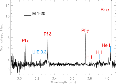
Figure 1: VLT/ISAAC spectrum of PN M 1-20. The atomic H lines of the Pfund series (Pf_ϵ, Pf_δ and Pf_γ), H I (6-17), H I (6-15) and Br_α as well as the UIE feature at 3.3 $\mu$m and the line of He I (4-5) are indicated.

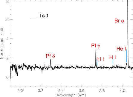
Figure 2: VLT/ISAAC spectrum of Tc 1. The atomic H lines of the Pfund series (Pf_δ and Pf_γ), H I (6-17), H I (6-15) and Br_α, as well as the line of He I (4-5) are indicated.

3 The 3.3 $\mu$m UIE feature

We clearly detect the 3.3 $\mu$m UIE feature in M 1-20, while this feature is completely lacking in Tc 1. This is consistent with the Spitzer spectra; M 1-20 displays UIE features (PAH-like) at 6.2, 7.7, 8.6 and 11.3 $\mu$m, but these are absent in Tc 1 (e.g., García-Hernández et al. 2010). The detected UIE feature in the M 1-20 spectrum was fitted with a Gaussian to determine the feature’s FWHM and central wavelength. Due to the emission line of H I (Pf_δ) at 3.32 $\mu$m, it was necessary to deblend both features. The average central wavelength of the UIE feature was 3.31 $\mu$m, with a FWHM of 0.05 $\mu$m. This is consistent with the values measured by Tokunaga et al. (1991) and Smith & McLean (2008) (average values of $\lambda$_c $\sim$3.29 $\mu$m and FWHM $\sim$0.04 $\mu$m) in extended objects such as PNe, (proto-) PNe, and H II regions. In Figure 1, we can see the 3.3 $\mu$m UIE feature in the M 1-20 spectrum blended with the Pf_δ hydrogen emission line at 3.32 $\mu$m.

3.1 Possible carriers of the 3.3 $\mu$m UIE feature

The 3.3 $\mu$m feature belongs to the group of UIE features or aromatic infrared bands (AIBs) at 3.3, 6.2, 7.7, 8.6, 11.3 and 12.7 $\mu$m. These bands may be accompanied by aliphatic bands at 3.4, 6.9 and 7.3 $\mu$m and unassigned features at 15.8, 16.4, 17.4, 17.8 and 18.9 $\mu$m (Jourdain de Muizon et al. 1990; Kwok et al. 1999; Chiar et al. 2000; Sturm et al. 2000; Sellgren et al. 2007), and the broad emission features at $\sim$6-9, 9-13, 15-20, and 25-35 $\mu$m, which are believed to be produced by a carbonaceous mixture of aromatic and aliphatic structures (e.g., HAC, coal, petroleum fractions, etc.) and/or their decomposition products (García-Hernández et al. 2010, 2012; Kwok & Zhang 2011). The 11.3 $\mu$m UIE feature is found to be correlated with the 3.3 $\mu$m feature (Russell et al. 1977), suggesting a common origin for the two features. This correlation holds for fullerene PNe; we detect the weak UIE feature at 3.3 $\mu$m in our VLT/ISAAC spectrum and the M 1-20 Spitzer spectrum shows a very strong aromatic-like infrared band at 11.3 $\mu$m (García-Hernández et al. 2012), while Tc 1 displays a very weak emission at 11.3 $\mu$m and it does not show the feature at 3.3 $\mu$m.

A wide variety of molecules have been proposed as possible carriers of these 3.3 and 11.3 $\mu$m UIE bands. Nowadays, the most accepted idea is that they originate from the C-H vibration modes of aromatic compounds or PAHs (e.g., Duley & Williams 1981; Leger & Puget 1984; Allamandola, Tielens & Barker 1985). However, Sadjadi et al. (2015) calculated the out-of-plane (OOP) bending mode frequencies of 60 neutral PAH molecules and found that it is difficult to fit the 11.3 $\mu$m UIE feature. This feature cannot be fitted by superpositions of pure PAH molecules and O- (and or Mg-) containing species are needed to achieve a good fit, suggesting that the PAHdb model (Bauschlicher et al. 2010; Boersma et al. 2014) has difficulties to explain the UIE phenomenon (see Sadjadi et al. 2015 for more details). Maltseva et al. (2015) also found difficulties for predicting high-resolution experimental absorption spectra of PAHs in the 3-$\mu$m region with harmonic density functional theory (DFT) calculations. Finally, Gadallah et al. (2013) also found that the 3.3 $\mu$m and 6.2 $\mu$m AIBs are also clearly observed in the spectrum of heated HAC dust.

On the other hand, Duley & Williams (2011) suggest a model in which the astronomical emission at 3.3 $\mu$m can be explained by the heating of HAC dust via the release of stored chemical energy. This energy would be sufficient to heat dust grains (with sizes of $\sim$50-1000 Å) to temperatures at which they can emit at 3.3 $\mu$m. This alternative to the PAH hypothesis involves a solid material with a mix of aliphatic and aromatic structures (i.e., HACs), which may explain the broad emission features at $\sim$6-9, 9-13, 15-20, and 25-35 $\mu$m detected in PNe with fullerenes (García-Hernández et al. 2010, 2012) and most C-rich proto-PNe. Moreover, laboratory experiments show that the products of destruction of HAC grains are PAHs and fullerenes (Scott et al. 1997), something that could explain the detection of both types of molecules in some fullerene PNe (García-Hernández et al. 2010). Unfortunately, our VLT/ISAAC observations do not add much information about the real carrier (e.g., PAHs vs. HACs) of the 3.3 $\mu$m emission. The non-detection of 3.3 $\mu$m emission in Tc 1 may suggest a different spatial distribution of the 3.3 $\mu$m carrier and the C₆₀ (and C₇₀) fullerenes. Bernard-Salas et al. (2012) already found that the Spitzer C₆₀ 8.5 $\mu$m and weak 11.2 $\mu$m emission (which likely share the same carrier with the 3.3 $\mu$m emission, see above) are extended but they peak at opposite directions from the Tc 1 central star. The Spitzer observations (slit of $\sim$4” x 57” at a P.A. of 0 degrees) show extended emission up to $\sim$22” (Bernard-Salas et al. 2012), while our VLT/ISAAC spectra, taken with a smaller slit of 0.6 arcsec, show no extended emission at 3.3 $\mu$m. Thus, it could be possible that we miss the weak 3.3 $\mu$m emission in the ISAAC observations (e.g., a small column density throughout the circumstellar envelope). In the case of the more compact (apparent size of $\sim$2 arcsec) PN M 1-20 we have no spatial information from the Spitzer spectra (which covered the entire nebula) and the 3.3 $\mu$m emission in the VLT/ISAAC spectra is not extended.

In short, still it is not clear if the emission bands at 3.3 and 11.3 $\mu$m seen in PNe with fullerenes are only due to pure aromatic compounds or to mixed aromatic/aliphatic structures such as those of HAC-like dust.

4 Non detection of the fullerane features

The IR laboratory spectra (R$\sim$500) of several fulleranes such as C₆₀H₁₈, C₆₀H₃₆ or C₇₀H₃₈ (Iglesias-Groth et al. 2012), show that the strongest features in the mid-IR (2-20 $\mu$m) are those at $\sim$3.44, 3.51 and 3.54 $\mu$m (see Figure 3), being the best IR bands for searching these molecules in the circumstellar environments of fullerene-rich PNe. Thus, at the resolution (R$\sim$600) of the VLT/ISAAC observations it is possible to easily resolve these bands as well as to distinguish them from the 3.3 $\mu$m emission (Iglesias-Groth et al. 2012). However, none of these three emission features is detected in our VLT/ISAAC spectra of Tc 1 and M 1-20. Figure 3 shows the non-detection of the fullerane features between 3.4 and 3.6 $\mu$m in our VLT/ISAAC spectra of Tc 1 and M 1-20. The laboratory spectra of the fulleranes C₆₀H₁₈, C₇₀H₃₈ and C₆₀H_x+C₇₀H_y (see below) are also displayed and their corresponding 3.4-3.6 $\mu$m features are marked.

We could estimate approximate upper limits to the fluxes of the hydrogenated fullerene features (see Table 3). In order to obtain 2$\sigma$ upper limits to the expected emission line fluxes of the fullerane features at $\sim$3.5 $\mu$m, we measure the rms in our flux calibrated VLT/ISAAC spectra; rms values of $\sim$4.28 $\times$ 10^-19 ergcm^-2s^-1Å^-1 and $\sim$6.65 $\times$ 10^-18 ergcm^-2s^-1Å^-1 for Tc 1 and M 1-20 are obtained, respectively. Then we multiply these values by the widths (FWHMs in the range 0.02-0.10 $\mu$m) of the fullerane bands measured in the infrared laboratory spectra. We have used the laboratory spectra of two C₆₀H₁₈ isomers (obtained using hydrogen iodide and direct hydrogenation with metal hydrides), two C₆₀H₃₆ spectra at $+$48^∘C and $+$250^∘C, two C₇₀H₃₈ spectra at $+$50^∘C and $+$160^∘C, and the fullerane mixture 77 % of C₆₀H_x and 22 % C₇₀H_y with x $\approx$ y $\geq$ 30 at $+$45^∘C (see Iglesias-Groth et al. 2012 for more details). Finally, we divided these fluxes by the area ($\sim$0.6” arcsec² for both PNe) of the emission in the 3$-$4 $\mu$m range covered by our ISAAC observations.

Figure 3: VLT/ISAAC spectra of M 1-20 and Tc 1 in comparison with the laboratory spectra of the fulleranes C₆₀H₁₈, C₇₀H₃₈, and C₆₀H_x+C₇₀H_y in the 3.1-3.8 $\mu$m range. Note that the C₆₀H₁₈ fullerane bands at 3.42, 3.46, and 3.51 $\mu$m and the C₇₀H₃₈ fullerane bands at 3.44, and 3.54 $\mu$m are marked with dashed lines. The C₆₀H_x+C₇₀H_y fullerane bands are those at 3.44, 3.51, and 3.54 $\mu$m.

Table 3: Summary table showing examples of the expected fluxes for the fullerane features. Quoted values are the measured central wavelengths of the fullerane features, the full widths at half maximum (FWHM), the 2$\sigma$ upper detection limits to the expected emission line fluxes in Tc 1 and M 1-20, and the predicted fluxes for the fullerane bands.

Fullerane	$\lambda$c	FWHM	FLUX (Tc 1)	Predicted fluxes (Tc 1)	FLUX (M 1-20)	Predicted fluxes (M 1-20)
	($\mu$m)	(10-2$\mu$m)	(10-16ergcm-2s-1/”2)	(10-14ergcm-2s-1/”2)	(10-15ergcm-2s-1/”2)	(10-13ergcm-2s-1/”2)
C60H18 (isomer 1)	3.42	2.1	$\leq$3.00	9.43	$\leq$4.65	2.39
	3.46	3.6	$\leq$5.13	10.20	$\leq$7.98	2.58
	3.51	5.1	$\leq$7.28	13.25	$\leq$11.30	3.36
C60H18 (isomer 2)	3.42	2.2	$\leq$3.13	12.74	$\leq$4.87	1.42
	3.45	3.4	$\leq$4.85	13.92	$\leq$7.53	1.56
	3.51	5.5	$\leq$7.85	18.21	$\leq$12.18	2.06
C60H36 (+48∘C)	3.44	2.3	$\leq$3.33	22.13	$\leq$5.18	5.58
	3.54	7.7	$\leq$11.02	16.23	$\leq$17.10	4.11
C60H36 (+250∘C)	3.44	2.2	$\leq$3.10	30.11	$\leq$4.80	3.39
	3.53	10.1	$\leq$14.38	22.08	$\leq$22.33	2.47
C70H38 (+50∘C)	3.44	2.5	$\leq$3.62	18.13	$\leq$5.63	4.61
	3.54	7.0	$\leq$10.05	16.75	$\leq$15.62	4.22
C70H38 (+160∘C)	3.44	2.5	$\leq$3.55	1.81	$\leq$5.52	2.72
	3.54	6.3	$\leq$8.97	1.68	$\leq$13.93	2.56
C60Hx+C70Hy (+45∘C)	3.44	2.2	$\leq$3.13	20.13	$\leq$4.87	5.08
	3.51	2.8	$\leq$4.00		$\leq$6.20
	3.54	2.5	$\leq$3.57	18.71	$\leq$5.53	4.75

On the other hand, by using the molar absorptivity values for the fullerenes and fulleranes reported by Iglesias-Groth et al. (2011, 2012), we may estimate the predicted fluxes for the fullerane features in Tc 1 and M 1-20 (see Table 3). By taking the molar absorptivity ratio (e.g., $\epsilon$_C60/$\epsilon$_fulleranes) of the fullerene and fullerane bands and the observed fluxes of the C₆₀ and C₇₀ infrared bands less contaminated by other species (García-Hernández et al. 2012) we estimate the expected flux of the fullerane features at $\sim$3.5 $\mu$m. It is to be noted here that this is only an approximation and a complete model for the excitation/emission of both species should be needed. The Spitzer integrated fluxes of the infrared bands at 8.5 and 17.4 $\mu$m (C₆₀), and 14.9 $\mu$m (C₇₀) were taken from García-Hernández et al. (2012) and converted to flux/arcsec² by considering the area covered by the fullerenes emission in the Spitzer spectra of Tc 1 ($\sim$80 arcsec² at 8.5 $\mu$m and $\sim$53 arcsec² at 14.9 and 17.4 $\mu$m) and M 1-20 ($\sim$4 arcsec² at 8.5, 14.9, and 17.4 $\mu$m).

Table 3 shows some examples of the estimated 2$\sigma$ upper limits and the predicted fluxes for the fullerane bands. For example, the molar absorptivity ratio of the C₆₀H₃₆ band at 3.44 $\mu$m and the C₆₀ infrared band at 8.5 $\mu$m is $\epsilon$_8.5/$\epsilon$_3.44$\sim$0.34. Thus, the expected flux of the C₆₀H₃₆ band at 3.44 $\mu$m in Tc 1 and M 1-20 would be $\sim$22.13 $\times$ 10^-14 ergcm^-2s^-1/arcsec² and $\sim$5.58 $\times$ 10^-13 ergcm^-2s^-1/arcsec², respectively (see Table 3). Similar values are obtained for the fullerane C₆₀H₃₆ band at 3.54 $\mu$m, with expected fluxes of $\sim$16.23 $\times$ 10^-14 ergcm^-2s^-1/arcsec², and $\sim$4.11 $\times$ 10^-13 ergcm^-2s^-1/arcsec² in Tc 1 and M 1-20, respectively. In summary, the expected fluxes for all fullerane bands of C₆₀H₁₈, C₆₀H₃₆, C₇₀H₃₈ and the mixture C₆₀H_x+C₇₀H_y (by using the observed Spitzer fluxes of the C₆₀ 8.5 and 17.4 $\mu$m and C₇₀ 14.9 $\mu$m bands) are in the range of $\sim$1.7-30 $\times$ 10^-14 and $\sim$1.4-5.6 $\times$ 10^-13 ergcm^-2s^-1/arcsec² in Tc 1 and M 1-20, respectively (see Table 3 for some representative examples).

By comparing the values of the predicted fluxes with our 2$\sigma$ upper limits (Table 3), we find that the expected fluxes are a factor of $\sim$20$-$1000 and $\sim$10$-$100 higher than the 2$\sigma$ upper limits for Tc 1 and M 1-20, respectively. From these estimations we thus conclude that if fulleranes are present in Tc 1 and M 1-20, then they seem to be by far less abundant than C₆₀ and C₇₀.

As we mentioned above, thermal heating via chemical reactions internal to HAC dust may explain the detection of fullerenes in the H-rich circumstellar environments of PNe and would potentially form fulleranes (Duley & Williams 2011). In addition, Duley & Hu (2012) reported that laboratory spectra of HAC nano-particles containing fullerene precursors (or proto-fullerenes; PFs), but not C₆₀, display the same set of mid-IR features as the isolated C₆₀ molecule. They suggest an evolutionary sequence for the conversion of HAC to fullerenes, in which initial HAC de-hydrogenation is followed by PFs formation and subsequent conversion of PFs to closed cage structures such as C₆₀. Under the Duley & Hu (2012) scenario, Tc 1 would represent the last stage in the HAC de-hydrogenation process (i.e., only fullerenes are present), while the proto-PN IRAS 01005$+$7910 would represent an intermediate stage where the PFs are being converted to fullerenes. Remarkably, fulleranes may be also by-products of this conversion from HAC to fullerenes (Duley & Hu 2012).

Interestingly, Zhang & Kwok (2013) have (tentatively) detected fulleranes in the proto-PN IRAS 01005$+$7910; three strong C-H stretching bands at 3.48, 3.51, and 3.58 $\mu$m are apparently present in its ISO spectrum with fluxes comparable to the one of the 3.3 $\mu$m feature. By assuming that all features have the same oscillator strength, they conclude that the calculated relative strengths indicate that the m value (degree of hydrogenation of the fulleranes C₆₀H_m) may lie within the range from 25-40, which is consistent with the production of C₆₀H₃₆ (the dominant product of the hydrogenation reaction of C₆₀; e.g., Cataldo & Iglesias-Groth 2009). In addition, the observed fluxes of the C₆₀ and fullerane bands suggest that about 50 percent of fullerenes have been hydrogenated. Curiously, IRAS 01005$+$7910 exceptionally displays very strong C₆₀⁺ DIBs (Iglesias-Groth & Esposito 2013).

Our non-detection of fulleranes in more evolved PNe (such as Tc 1 and M 1-20 with T_eff$>$ 30,000 K) together with their possible detection in less evolved sources (like IRAS 01005$+$7910 with T_eff$\sim$21,500 K) thus suggest that fulleranes may be formed in the short transition phase between AGB stars and PNe but they are quickly destroyed; e.g., photochemically processed by the rapidly changing UV radiation from the central star. The rapid increase of the UV radiation towards the PN stage will easily break the C$-$H bonds of the previously formed fullerane molecules, forming fulleranes at lower hydrogenation degree or forming back - more resistant - C₆₀ and C₇₀ fullerenes and molecular hydrogen (Cataldo & Iglesias-Groth 2009). However, still it is not clear what is the origin of fulleranes. Fulleranes could be formed via the Duley & Hu (2012) HAC de-hydrogenation process mentioned above in which fulleranes may be by-products of the conversion from PFs to C₆₀ or they could be formed by the reaction of pre-existing fullerenes (e.g., formed by the photochemical processing of HACs; Scott et al. 1997) with atomic hydrogen. During the short ($\sim$10²-10⁴ years) transition phase AGB-PN, H₂ may be photodissociated into atomic H due to the gradual increase of the UV radiation field with the evolution of the central star and/or by shocks (H₂ dissociated through collisions) due to the fast post-AGB stellar winds. By reacting with atomic hydrogen fullerenes form fulleranes at various degree of hydrogenation. Thus, the post-AGB phase would make the reaction between fullerenes and atomic H more favorable (Cataldo & Iglesias-Groth 2009) and it seems to provide the right conditions for fullerane formation and detection.

5 Conclusions

We have presented VLT/ISAAC 2.9-4.1 $\mu$m spectroscopy of two fullerene PNe in our Galaxy. The spectrum of Tc 1 shows a continuum with no signs of UIE features and only H (and He) nebular lines. This indicates that the IR bands seen in the Tc 1 Spitzer spectrum are very likely due to C₆₀ and C₇₀ solely, and not other kind of molecules such as fulleranes or fullerene/PAH adducts. The M 1-20 VLT/ISAAC spectrum shows H and He nebular lines in conjunction with the UIE feature at 3.3 $\mu$m.

The VLT/ISAAC and Spitzer spectra of these fullerene PNe confirm a correlation between the 3.3 and 11.3 $\mu$m UIE features previously reported in the literature, which suggests a common carrier for these two features. Unfortunately, the VLT/ISAAC observations presented here cannot reveal the nature of the real carrier (e.g., PAHs vs. HACs) of the 3.3 $\mu$m emission.

Interestingly, we have reported the non-detection of the strongest bands of hydrogenated fullerenes (fulleranes such as C₆₀H₁₈, C₆₀H₃₆, C₇₀H₃₈ and a fullerane mixture) at $\sim$3.44, 3.51 and 3.54 $\mu$m in the 3$-$4 $\mu$m spectra of the fullerene-containing PNe Tc 1 and M 1-20. From the comparison of the predicted fluxes of the fullerane bands with our 2$\sigma$ upper limits, we conclude that if fulleranes are present in both objects, then they seem to be by far less abundant than isolated fullerene molecules.

Our non-detection of fulleranes in two fullerene PNe together with their possible detection (if real) in the fullerene proto-PN IRAS 01005$+$7910 suggest that these fullerene-related species may be formed in the short transition phase AGB$-$PN but they are rapidly destroyed; e.g., by the quick increase of the UV radiation from the central star towards the PN stage. The transition between AGB stars and PNe seems to be the best evolutionary stellar phase for finding fulleranes in space and 3$-$4 $\mu$m spectroscopy in a larger sample of C-rich proto-PNe is encouraged.

- (1) Allamandola, L. J., Tielens, A. G. G. M., & Barker, J. R. 1985, ApJ, 290, L25
- (2) Bauschlicher, C. W., Boersma, C., Ricca, A. et al. 2010, ApJS, 189, 341
- (3) Beaulieu, S. F., Dopita, M. A., & Freeman, K. C. 1999, ApJ, 515, 610
- (4) Bernard-Salas, J., Cami, J., Peeters, E. et al. 2012, ApJ, 757, 41
- (5) Boersma, C., Bauschlicher, C. W., Ricca, A. et al. 2014, ApJS, 211, 8
- (6) Cami, J. et al. 2010, Science, 329, 1180
- (7) Cataldo, F., & Iglesias-Groth, S. 2009, MNRAS, 400, 291
- (8) Cataldo, F., García-Hernández, D. A., & Manchado, A. 2014, Eur. Chem. Bull., 3, 740
- (9) Cataldo, F., García-Hernández, D. A., & Manchado, A. 2015, FNCN, 23, 818-823
- (10) Chiar, J. E., Tielens, A. G. G. M., Whittet, D. C. B. et al. 2000, ApJ, 537, 749
- (11) Cox, N. L. J. 2011, in PAHs and the Universe: A Symposium to Celebrate the 25th Anniversary of the PAH Hypothesis, EAS Publication Series Vol. 46, 349-354, eds Joblin, C. & Tielens, A. G. G. M.
- (12) Cutri, R. M. et al. 2012, VizieR On-line Data Catalog: II/311
- (13) De Bruijne, J. H. J., & Eilers, A. -C. 2012, A&A, 546, A61
- (14) Díaz-Luis, J. J., García-Hernández, D. A., D. A., Rao, N. K. et al. 2015, A&A, 573, A97
- (15) Duley, W. W., & Williams, D. A. 1981, MNRAS, 196, 269
- (16) Duley, W. W., & Williams, D. A. 2011, ApJ, 737, L44
- (17) Duley, W. W., & Hu, A. 2012, ApJ, 745, L11
- (18) Gadallah, K. A. K., Mutschke, H., & Jager, C. 2013, A&A, 554, A12
- (19) García-Hernández, D. A., Manchado, A., García-Lario, P. et al. 2010, ApJ, 724, L39
- (20) García-Hernández, D. A., Iglesias-Groth, S., Acosta-Pulido, J. A. et al. 2011a, ApJ, 737, L30
- (21) García-Hernández, D. A., Rao, N. K., & Lambert, D. L. 2011b, ApJ, 729, 126
- (22) García-Hernández, D. A., Villaver, E., García-Lario, P. et al. 2012, ApJ, 760, 107
- (23) García-Hernández, D. A., Cataldo, F., & Manchado, A. 2013, MNRAS, 434, 415
- (24) García-Hernández, D. A., & Díaz-Luis, J. J. 2013, A&A, 550, L6
- (25) García-Lario, P., Manchado, A., Ulla, A., Manteiga, M. 1999, ApJ, 513, 941
- (26) Gudennavar, S. B., Bubbly, S. G., Preethi, K. et al. 2012, ApJ, 199, 8
- (27) Iglesias-Groth, S. 2007, ApJ, 661, L167
- (28) Iglesias-Groth, S., Cataldo, F., & Manchado, A. 2011, MNRAS, 413, 213
- (29) Iglesias-Groth, S., García-Hernández, D. A., Cataldo, F. et al. 2012, MNRAS, 423, 2868
- (30) Iglesias-Groth, S., & Esposito, M. 2013, ApJ, 776, L2
- (31) Jourdain de Muizon, M., D’Hendecourt, L. B., & Geballe, T. R. 1990, A&A, 227, 526
- (32) Kroto, H. W., Heath, J. R., Obrien, S. C. et al. 1985, Nature, 318, 162
- (33) Kwok, S., Volk, K., & Hrivnak, B. J. 1989, ApJ, 345, L51
- (34) Kwok, S., Volk, K., & Hrivnak, B. J. 1999, A&A, 350, L35
- (35) Kwok, S., & Zhang, Y. 2011, Nature, 479, 80
- (36) Leger, A., & Puget, J. L. 1984, A&A, 137, L5
- (37) Maltseva, E., Petrignani, A., Candian, A. et al. 2015, eprint arXiv:1510.04948
- (38) Otsuka, M., Kemper, F., Cami, J. et al. 2014, MNRAS, 437, 2577
- (39) Russell, R. W., Soifer, B. T., & Merrill, K. M. 1977, ApJ, 213, 66
- (40) Sadjadi, S. A., Zhang, Y., & Kwok, S. 2015, ApJ, 807, 95
- (41) Scott, A., Duley, W. W., & Pinho, G. P. 1997, ApJ, 489, L193
- (42) Sellgren, K., Uchida, K. I., & Werner, M. W. 2007, ApJ, 659, 1338
- (43) Sellgren, K., Werner, M. W., Ingalls, J. G. et al. 2010, ApJ, 722, L54
- (44) Smith, E. C. D., & McLean, I. S. 2008, ApJ, 676, 408
- (45) Soubiran, C., Jasniewicz, G., Chemin, L. et al. 2013, A&A, 552, A64
- (46) Sturm, E., Lutz, D., Tran, D. et al. 2000, A&A, 358, 481
- (47) Tokunaga, A. T., Sellgren, K., Smith, R. G. et al. 1991, ApJ, 380, 452
- (48) Volk, K., Hrivnak, B. J., Matsuura, M. et al. 2011, ApJ, 735, 127
- (49) Wang, W., & Liu, X. -W. 2007, MNRAS, 381, 669
- (50) Webster, A. 1995, MNRAS, 277, 1555
- (51) Wegner, W. 2003, AN, 324, 219
- (52) Williams, R., Jenkins, E. B., Baldwin, J. A. et al. 2008, ApJ, 677, 1100
- (53) Zhang, Y., & Kwok, S. 2011, ApJ, 730, 126
- (54) Zhang, Y., & Kwok, S. 2013, Earth, Planets and Space, 65, 1069