Templates and subtemplates of Rössler attractors from a bifurcation diagram

Abstract

We study the bifurcation diagram of the Rössler system. It displays the various dynamical regimes of the system (stable or chaotic) when a parameter is varied. We choose a diagram that exhibits coexisting attractors and banded chaos. We use the topological characterization method to study these attractors. Then, we details how the templates of these attractors are subtemplates of a unique template. Our main result is that only one template describe the topological structure of height attractors. This leads to a topological partition of the bifurcation diagram that gives the symbolic dynamic of all bifurcation diagram attractors with a unique template.

Keywords: Rössler system, bifurcation diagram, template, subtemplate

1 Introduction

Since 1976, the Rössler system [1] is well know for it’s simplicity (three differential equations with only one non linear term) and its dynamical richness producing chaos. Used as a basic system to demonstrate various properties of dynamical systems, this system is still a source inspiration for researchers. This system has been widely explored with several tools. The main goal of this paper is to extend the use of the topological characterization method to several chaotic attractors. We introduce a way to use the template as a global description that contains various attractors templates of the Rössler system.

In this paper, we will study this system in a parameter space to highlight common properties of neighbours attractors in this space. Castro et al. [2] study of the parameter space of this system using Lyapunov exponents reflects its dynamics (stable, chaotic or trajectory diverging). The maps are built varying parameters $a$ and $c$ of the system. These maps display fractal structure and illustrate period doubling cascades. This principle is also employed by Barrio et al. [3] for the three parameters of the Rössler system. Their analysis of local and global bifurcations of limit cycles permits to a have a better understanding of the parameter space. Additionally, attractors with equilibrium points associated to their first return maps are also plotted to illustrate the various dynamics of this system, including coexistence of attractors. To enlarge this overview of recent work on the bifurcations and dynamics on the Rössler system, Genesio et al. [4] use the first-order harmonic balance technique to study fold, flip and Neimark-Sacker bifurcations in the whole parameter space. Finally, the recent work of Sprott & Li [5] introduce another way to reach coexisting attractors in addition to the cases identified by Barrio et al. [3].

In this paper we study a bifurcation diagram of the Rössler system exhibiting various dynamics using topological properties of attractors. We use the topological characterization method based on the topological properties of the attractor’s periodic orbits [6]. The purpose is not only to obtain templates of chaotic attractors but also to find common points or properties as it as already been shown for this system by Letellier et al. [7] for a “funnel attractor”. In this particular case, a linking matrix describes the template depending on the number of branches. In this paper, we will explore a bifurcation diagram and show that only one template contains all the templates of attractors as subtemplates.

This paper is organized as follow. The first part introduces the Sprott & Li [5] work with their bifurcation diagram. The second part details the topological characterization method; height attractors are studied and their templates are obtained. Then we prove that the eight templates are subtemplates of a unique template. It describes the topological structure of all the attractors of the entire bifurcation diagram. Finally we provide a partition of the bifurcation diagram giving the symbolic dynamic associated with the unique template depending on the bifurcation parameter.

2 Bifurcation diagram

Barrio et al. [3] highlight the fact that a Rössler system can have to coexisting attractors as solutions for a set of parameters. Sprott & Li [5] parametrize the Rössler system [1] with the parameter $\alpha$

$$\left\{\begin{aligned} \dot{x}&=-y-z\\ \dot{y}&=x+ay\\ \dot{z}&=b+z(x-c)\end{aligned}\right.\text{ with }\left\{\begin{aligned} a&=0.2+0.09\alpha\\ b&=0.2-0.06\alpha\\ c&=5.7-1.18\alpha\end{aligned}\right.$$ (1)

in order to explore bifurcations. When $\alpha=1$, two attractors coexist in the phase space. We reproduce their bifurcation diagram when $\alpha$ varies. The value of the fixed points of the system are

$$S_{\pm}=\left|\begin{array}[]{l}\displaystyle x_{\pm}=\frac{c\pm\sqrt{c^{2}-4ab}}{2}\\[8.5359pt] \displaystyle y_{\pm}=\frac{-c\mp\sqrt{c^{2}-4ab}}{2a}\\[8.5359pt] \displaystyle z_{\pm}=\frac{c\pm\sqrt{c^{2}-4ab}}{2a}\,.\end{array}\right.$$ (2)

The bifurcation diagram Fig. 1 is obtained using the following Poincaré section

$$\mathcal{P}\equiv\left\{(y_{n},-z_{n})\in\mathbb{R}^{2}\ |-x_{n}=-x_{-}\right\}$$ (3)

where $x_{-}$ is the $x$ value of the fixed point $S_{-}$ (see [8] for details on this Poincaré section). The uses of this Poincaré section explains why Fig. 1 is similar to FIG. 4 of [5]: we use $y_{n}$ and they use $M$ which is a local maximum of $x$. Consequently, in both case, values close to zero correspond to value close to the center of the attractor and oppositely, high absolute values correspond to the outside boundary of the attractor.

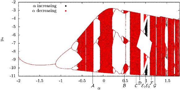
Figure 1: Bifurcation diagram when $\alpha$ varies: $\alpha$ increasing (red) and $\alpha$ decreasing (black). This figure reproduces the FIG. 4 of [5]. Using $\alpha$ increasing or decreasing replaces different initial conditions used in the original paper [5]. $\mathcal{A}$, $\mathcal{B}$, $\mathcal{C}$, $\mathcal{D}$, $\mathcal{E}_{1}$, $\mathcal{E}_{2}$, $\mathcal{F}$ and $\mathcal{G}$ refers to attractors solutions with the parameters indicated in (4).

This diagram indicates parameter for the Rössler system where the solution is a limit cycle or chaotic. This diagram exhibits a doubling period cascade that is a classical route to chaos for $-2<\alpha<0.2$. This is followed by a chaotic puff ($\alpha=0.5$) and by various regimes (banded chaos and almost fully developed chaos). We chose representative values of $\alpha$ where one ore two attractors are solutions of the system

$$\begin{array}[]{ll|ll}\mathcal{A}&\alpha=-0.25&\mathcal{E}_{1}&\alpha=1\\ \mathcal{B}&\alpha=0.5&\mathcal{E}_{2}&\alpha=1\\ \mathcal{C}&\alpha=0.78&\mathcal{F}&\alpha=1.135\\ \mathcal{D}&\alpha=0.86&\mathcal{G}&\alpha=1.22\;.\end{array}$$ (4)

We analyse these attractors using topological characterization method in order to obtain a generic description of the attractors while $\alpha$ is varied.

3 Topological characterization

The main purpose of the topological characterization method is to build a template using topological properties of periodic orbits. The template has been introduced by [9, 10] further to the works of Poincaré [11]. According to Ghrist et al. [12], a template is a compact branched two-manifold with boundary and smooth expansive semiflow built locally from two type of charts: joining and splitting. Each charts carries a semiflow, endowing the template with an expanding semiflow, and the gluing maps between charts must respect the semiflow and act linearly on the edges. This topological characterization method is detailed by Gilmore & Lefranc [13, 6]. Recently, we detail additional conventions to obtain templates that can be compared and sorted [14, 15]. We start with a brief description of the method. As the trajectories are chaotic, they are unpredictable in a long term behavior. But attractors have a time invariant global structure where its orbits compose its skeleton. The purpose of the method is to use the topological properties of these orbits to describe the structure of the attractor. We provide a sum up of this method with eight steps (including our conventions):

1. Display the attractor with a clockwise flow;

2. Find the bounding torus;

3. Build a Poincaré section;

The first step permits to ensure that the study will be carried out to the respect of conventions: clockwise flow having a clockwise toroidal boundary and described by a clockwise template. This clockwise convention ensures us to describe template with a unique linking matrix, a keystone to work only with linking matrices [14]. The toroidal boundary give a global structure that permit to classify attractors. For a given toroidal boundary, a typical Poincaré section is associated according to the Tsankov & Gilmore theory [16]. This Poincaré section contains one or more components to permit an effective discretization of trajectories and consequently an efficient partition of the attractor.

1. Compute the first return map and define a symbolic dynamic;

2. Extract and encode periodic orbits;

3. Compute numerically the linking numbers between couple of orbits;

The first return map details how two consecutive crossings of a trajectory through the Poincaré section are related and permits to associate a symbol to each point. It permits to define a partition of the attractor and a symbolic dynamic. Associated symbols depend on the parity of the slope (even for the increasing one, odd for the other). Up to this point, periodic orbits structuring the attractor are extracted and encoded using this symbolic dynamic. The linking number between a pair of orbits is a topological invariant indicating how orbits are wind one around another. In this paper, we use the orientation convention of Fig. 2.

Convention		Permutations		Torsions
$+1$	$-1$	positive	negative	positive	negative

Figure 2: Convention representation of oriented crossings. The permutation between two branches is positive if the crossing generated is equal to $+1$, otherwise it is a negative permutation. We use the same convention for torsions.

The final steps concern the template:

1. Propose a template;

2. Validate the template with the theoretical computation of linking numbers.

The template is clockwise oriented. The template of an attractor bounded by genus one torus is defined by a unique linking matrix. This matrix describes how branches are torn and permuted. We use the Melvin & Tufillaro [17] standard insertion convention: when the branches stretch and squeeze, the left to the right order of the branches corresponds to the bottom to top order. The diagonal elements of the matrix indicate the torsions of branches and off diagonal elements give the permutations between two branches. Finally, to validate a template, we use a procedure introduced by Le Sceller et al. [18] that permits to compute linking numbers theoretically from a linking matrix. Linking numbers obtained theoretically with this method have to correspond with those obtained numerically at the step (vi) to validate the template. The challenge of this procedure resides in the step (vii) because it is non trivial to find a template whose theoretical linking numbers correspond to the numerically computed linking numbers.

3.1 Attractor $\mathcal{A}$

In this section we will detail the previously described procedure step by step for attractor $\mathcal{A}$.

1. Display the attractor with a clockwise flow;

We propose to make a rotation of the attractor around the $y$-axis. Displaying the attractor in the phase space $(-x,y)$, the flow evolves clockwise (Fig. 3a).

1. Find the bounding torus;

The attractor is bounded by a genus one torus: a surface with only one hole. Consequently, a Poincaré section with one-component is required.

1. Build a Poincaré section;

We build our Poincaré section using $x_{-}$ (2)

$$\mathcal{P}\equiv\left\{(y_{n},-z_{n})\in\mathbb{R}^{2}\ |-x_{n}=-x_{-}\right\}\;.$$ (5)

This Poincaré section is a half-plan transversal to the flow as illustrated in grey Fig. 3a.

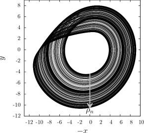
(a) Chaotic attractor $\mathcal{A}$		(b) First return map

Figure 3: (a) Chaotic attractor $\mathcal{A}$ solution to the equation (1). Parameter value $\alpha=-0.25$ with the initial conditions $x=-1.25$, $y=-0.72$ and $z=-0.1$. (b) First return map to the Poincaré section (5) using $\rho_{n}$ (the arrow indicates the orientation).

1. Compute the first return map and define a symbolic dynamic;

To compute the first return map, we first normalize the intersection value of the flow through the Poincaré section: $\rho_{n}$. This value is oriented from the inside to the outside (Fig. 3a). Then the first return map is obtained by plotting $\rho_{n+1}$ versus $\rho_{n}$ (Fig. 3b). This return map is the classical unimodal map made of an increasing branch followed by a decreasing one. This first return map indicates that the classical “horseshoe” mechanism generate this chaotic attractor. The symbolic dynamic is defined as follow: “$0$” for the increasing branch and “$1$” for the decreasing one.

1. Extract and encode periodic orbits;

Using, the first return map, we can locate periodic orbits that the flow visits while it covers the attractor. For instance, there is only one period one orbit because the bisector cross the map once. We extract five orbits with a period lower than six: $1$, $10$, $1011$, $10110$ and $10111$ (Fig. 4).

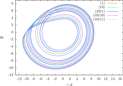
Figure 4: Orbits of the chaotic attractor $\mathcal{A}$.

1. Compute numerically the linking numbers;

We compute linking numbers between each pair of periodic orbits. The linking number between a pair of orbits is obtained numerically (Tab. 1).

Table 1: Linking numbers between pairs of orbits extracted from the symmetric chaotic attractor $\mathcal{A}$.

	(1)	(10)	(1011)	(10110)
(10)	-1
(1011)	-2	-3
(10110)	-2	-4	-8
(10111)	-2	-4	-8	-10

1. Propose a template;

Using these linking numbers and the first return map structure, we propose the template (Fig. 5). This template is made of trivial part with a chaotic mechanism. The latter is composed by a splitting chart that separate continuously the flow into two branches. The left one encoded “$0$” permute negatively over the right one encoded “$1$”; the latter have a negative torsion. After the torsion and permutation, branches stretch and squeeze to a branch line using the standard insertion convention. This template is thus described by the linking matrix

$$T(\mathcal{A})=\left[\begin{array}[]{C{1.3em}C{1.3em}}\@add@centering&-1\@add@centering\cr-1\@add@centering&-1\@add@centering\end{array}\right\rsem\;.$$ (6)

Figure 5: $T_{\mathcal{A}}$: template of attractor $\mathcal{A}$.

1. Validate the template computing theoretically the linking numbers.

The theoretical calculus using the linking matrix and the orbits permits to obtain the same table of linking numbers. This validates the template of $\mathcal{A}$ defined by $T(\mathcal{A})$ (Fig. 5).

3.2 Attractors $\mathcal{B}$ to $\mathcal{G}$

In this section, we will only give the key steps for others attractors: $\mathcal{B}$, $\mathcal{C}$, $\mathcal{D}$, $\mathcal{E}_{1}$, $\mathcal{E}_{2}$, $\mathcal{F}$ and $\mathcal{G}$. We start with the Fig. 6 displaying these attractors for parameters (4) and with a clockwise flow evolution. We can observe that these attractors are made of fully developed chaos (Fig. 6acg) or banded chaos (Fig. 6bdf) or coexisting attractors of banded chaos (Fig. 6e).

(a) $\mathcal{A}$ for $\alpha=-0.25$	(b) $\mathcal{B}$ for $\alpha=0.5$	(c) $\mathcal{C}$ for $\alpha=0.78$
(d) $\mathcal{D}$ for $\alpha=0.86$	(e) $\mathcal{E}_{1}$ and $\mathcal{E}_{2}$ for $\alpha=1$	(f) $\mathcal{F}$ for $\alpha=1.135$
	(g) $\mathcal{G}$ for $\alpha=1.22$

Figure 6: Eight chaotic attractors for different values of $\alpha$ from the bifurcation diagram (Fig. 1)

All these attractors are bounded by a genus one torus. We use the Poincaré sections: (7) for $\mathcal{A}$, $\mathcal{C}$, $\mathcal{G}$, (8) $\mathcal{D}$, $\mathcal{E}_{1}$, $\mathcal{E}_{2}$, $\mathcal{F}$ and (9) for $\mathcal{B}$:

$$\mathcal{P}\equiv\left\{(y_{n},-z_{n})\in\mathbb{R}^{2}\ |-x_{n}=-x_{-}\right\}\ ,$$ (7)

$$\mathcal{P}\equiv\left\{(y_{n},-z_{n})\in\mathbb{R}^{2}\ |-x_{n}=-x_{-},\ -\dot{x}_{n}<0,y<-7\right\}\ ,$$ (8)

$$\mathcal{P}\equiv\left\{(y_{n},-z_{n})\in\mathbb{R}^{2}\ |-x_{n}=-x_{-},\ -\dot{x}_{n}<0,y<-9\right\}\;.$$ (9)

We compute the first return maps to these Poincaré sections using a normalized variable $\rho_{n}$ oriented from the inside to the outside of the boundary. The eight return maps (Fig. 7) are multimodal with differential points and the number of their branches are two, three or four. We chose a symbolic dynamic for each first return map with respect to the slope orientation of branches

$$\begin{array}[]{ll|ll}\mathcal{A}&0\ 1&\mathcal{E}_{1}&0\ 1\\ \mathcal{B}&0\ 1&\mathcal{E}_{2}&1\ 2\\ \mathcal{C}&0\ 1\ 2&\mathcal{F}&0\ 1\ 2\ 3\\ \mathcal{D}&0\ 1\ 2&\mathcal{G}&0\ 1\ 2\;.\end{array}$$ (10)

(a) $\mathcal{A}$ for $\alpha=-0.25$	(b) $\mathcal{B}$ for $\alpha=0.5$	(c) $\mathcal{C}$ for $\alpha=0.78$
(d) $\mathcal{D}$ for $\alpha=0.86$	(e1) $\mathcal{E}_{1}$ for $\alpha=1$	(e2) $\mathcal{E}_{2}$ for $\alpha=1$
(f) $\mathcal{F}$ for $\alpha=1.135$	(g) $\mathcal{G}$ for $\alpha=1.22$

Figure 7: First return maps of the eight attractors of the Fig. 6.

We extract a set of orbits for each attractors and numerically compute linking numbers between pairs of orbits (Tab. 2). Thus, we propose templates. They are validated using Le Sceller et al. procedure [18]. All the results are summed up in the Tab. 2.

Table 2: Linking numbers between pairs of orbits extracted from the attractors of Fig. 6 and their associated linking matrix describing their template.

	Linking numbers	Linking matrix
$\mathcal{A}$	(1) (10) (1011) (10110) (10) -1 (1011) -2 -3 (10110) -2 -4 -8 (10111) -2 -4 -8 -10	$T(\mathcal{A})=\left[\begin{array}[]{C{1.3em}C{1.3em}}\@add@centering&-1\@add@centering\\ -1\@add@centering&-1\@add@centering\end{array}\right\rsem$
$\mathcal{B}$	(1) (10) (1011) (10110) (10) -5 (1011) -10 -21 (10110) -13 -26 -52 (10111) -13 -26 -52 -65	$T(\mathcal{B})=\left[\begin{array}[]{C{1.3em}C{1.3em}}-6\@add@centering&-6\@add@centering\\ -6\@add@centering&-5\@add@centering\end{array}\right\rsem$
$\mathcal{C}$	(1) (10) (2010) (2011) (10) -1 (2010) -2 -3 (2011) -2 -3 -6 (1011) -2 -3 -6 -6	$T(\mathcal{C})=\left[\begin{array}[]{C{1.3em}C{1.3em}C{1.3em}}\@add@centering&-1\@add@centering&-1\@add@centering\\ -1\@add@centering&-1\@add@centering&-1\@add@centering\\ -1\@add@centering&-1\@add@centering&\@add@centering\end{array}\right\rsem$
$\mathcal{D}$	(1) (221) (211) (2221) (2211) (221) -4 (211) -4 -12 (2221) -5 -15 -15 (2211) -5 -15 -15 -20 (22110) -6 -18 -18 -24 -24	$T(\mathcal{D})=\left[\begin{array}[]{C{1.3em}C{1.3em}C{1.3em}}-4\@add@centering&-4\@add@centering&-4\@add@centering\\ -4\@add@centering&-3\@add@centering&-3\@add@centering\\ -4\@add@centering&-3\@add@centering&-2\@add@centering\end{array}\right\rsem$
$\mathcal{E}_{1}$	(1) (10) (1011) (101111) (10) -3 (1011) -6 -11 (101111) -9 -17 -34 (101110) -9 -17 -34 -51	$T(\mathcal{E}_{1})=\left[\begin{array}[]{C{1.3em}C{1.3em}}-2\@add@centering&-3\@add@centering\\ -3\@add@centering&-3\@add@centering\end{array}\right\rsem$
$\mathcal{E}_{2}$	(1) (21) (2111) (211111) (21) -3 (2111) -6 -11 (211111) -9 -17 -34 (212111) -9 -17 -34 -51	$T(\mathcal{E}_{2})=\left[\begin{array}[]{C{1.3em}C{1.3em}}-3\@add@centering&-3\@add@centering\\ -3\@add@centering&-2\@add@centering\end{array}\right\rsem$
$\mathcal{F}$	(3) (30) (31) (32) (313) (312) (322) (30) -3 (31) -3 -6 (32) -3 -6 -6 (313) -4 -9 -9 -8 (312) -4 -9 -9 -8 -12 (322) -4 -9 -9 -8 -12 -12 (332) -4 -9 -9 -8 -12 -12 -12	$T(\mathcal{F})=\left[\begin{array}[]{C{1.3em}C{1.3em}C{1.3em}C{1.3em}}-4\@add@centering&-4\@add@centering&-4\@add@centering&-4\@add@centering\\ -4\@add@centering&-3\@add@centering&-3\@add@centering&-3\@add@centering\\ -4\@add@centering&-3\@add@centering&-2\@add@centering&-3\@add@centering\\ -4\@add@centering&-3\@add@centering&-3\@add@centering&-3\@add@centering\end{array}\right\rsem$
$\mathcal{G}$	(1) (21) (2111) (2021) (21) -1 (2111) -2 -3 (2021) -2 -3 -6 (2110) -2 -3 -6 -6	$T(\mathcal{G})=\left[\begin{array}[]{C{1.3em}C{1.3em}C{1.3em}}\@add@centering&-1\@add@centering&-1\@add@centering\\ -1\@add@centering&-1\@add@centering&-1\@add@centering\\ -1\@add@centering&-1\@add@centering&\@add@centering\end{array}\right\rsem$

Only attractors $\mathcal{C}$ and $\mathcal{G}$ have the same template even if they have not the same orbits of period lower than five. The dynamic is not fully developed on each branch: some orbits are missing in both attractors compare to the full set of orbits. On the other hand, the two coexisting attractors have the same linking numbers but the orbits encode in two distinct ways. Their linking matrix are related as their template too. In fact, the orientation of the chaotic mechanism is the opposite one. This case permits to underline how orientation conventions are necessary to distinguish these two attractors.

4 Subtemplate

4.1 Algebraical relation between linking matrix

In this section, we will use some algebraic relation between linking matrix already defined in our previous papers [14, 15]. Here, we provide an overview of these relations. In the following description, a strip also nominates a branch of a branched manifold. First of all, a linker is a synthesis of the relative organization of $n$ strips: torsions and permutations in a planar projection (Fig. 2). A mixer is a linker ended by a joining chart that stretch and squeeze strips to a branch line. In the previous section, templates are only composed by one mixer defined by a linking matrix. We also define the concatenation of a torsion with a mixer and the concatenation of two mixers (see [14, 15] for more details). We remind that $\mathcal{X}$ designates the attractor, $T_{\mathcal{X}}$ its template and $T(\mathcal{X})$ the linking matrix that define its template. Using these algebraical relations between mixers and torsion, we can link the mixers of previously studied attractors:

$$\begin{array}[]{ll}T(\mathcal{C})=T(\mathcal{G})&\\[14.22636pt] T(\mathcal{E}_{1})=T(\mathcal{E}_{2})^{p}&\left[\begin{array}[]{C{1.3em}C{1.3em}}-3\@add@centering&-3\@add@centering\cr-3\@add@centering&-2\@add@centering\end{array}\right\rsem=\left[\begin{array}[]{C{1.3em}C{1.3em}}-2\@add@centering&-3\@add@centering\cr-3\@add@centering&-3\@add@centering\end{array}\right\rsem^{p}\\[14.22636pt] T(\mathcal{B})=[-5]\oplus T(\mathcal{A})&\left[\begin{array}[]{C{1.3em}C{1.3em}}-6\@add@centering&-6\@add@centering\cr-6\@add@centering&-5\@add@centering\end{array}\right\rsem=\left[\begin{array}[]{C{1.3em}C{1.3em}}-5\@add@centering&-5\@add@centering\cr-5\@add@centering&-5\@add@centering\end{array}\right]+\left[\begin{array}[]{C{1.3em}C{1.3em}}\@add@centering&-1\@add@centering\cr-1\@add@centering&-1\@add@centering\end{array}\right\rsem\\[14.22636pt] T(\mathcal{E}_{2})=[-2]\oplus T(\mathcal{A})&\left[\begin{array}[]{C{1.3em}C{1.3em}}-2\@add@centering&-3\@add@centering\cr-3\@add@centering&-3\@add@centering\end{array}\right\rsem=\left[\begin{array}[]{C{1.3em}C{1.3em}}-2\@add@centering&-2\@add@centering\cr-2\@add@centering&-2\@add@centering\end{array}\right]+\left[\begin{array}[]{C{1.3em}C{1.3em}}\@add@centering&-1\@add@centering\cr-1\@add@centering&-1\@add@centering\end{array}\right\rsem\end{array}$$ (11)

4.2 Subtemplates

A subtemplate is defined as follow by Ghrist et al. [12]: a subtemplate $\mathcal{S}$ of a template $\mathcal{T}$, written $\mathcal{S}\subset\mathcal{T}$, is a topological subset of $\mathcal{T}$ which, equipped with the restriction of a semiflow of $\mathcal{T}$ to $\mathcal{S}$, satisfies the definition of a template. For the eight attractors previously studied ($\mathcal{A}$, $\mathcal{B}$, $\mathcal{C}$, $\mathcal{D}$, $\mathcal{E}_{1}$, $\mathcal{E}_{2}$, $\mathcal{F}$ and $\mathcal{G}$) we will demonstrate that their templates are subtemplate of the template of $\mathcal{C}$ made of one mixer defined by

$$\left[\begin{array}[]{C{1.3em}C{1.3em}C{1.3em}}\@add@centering&-1\@add@centering&-1\@add@centering\cr-1\@add@centering&-1\@add@centering&-1\@add@centering\cr-1\@add@centering&-1\@add@centering&\@add@centering\end{array}\right\rsem\;.$$ (12)

Using the linking matrix defining $T_{\mathcal{A}}$ and $T_{\mathcal{C}}$, we directly find that $T(\mathcal{A})$ is a subset of $T(\mathcal{C})$ with the two first lines and columns

$$\left[\begin{array}[]{C{1.3em}C{1.3em}}\@add@centering&-1\@add@centering\cr-1\@add@centering&-1\@add@centering\end{array}\right\rsem\subset\left[\begin{array}[]{C{1.3em}C{1.3em}C{1.3em}}\@add@centering&-1\@add@centering&-1\@add@centering\cr-1\@add@centering&-1\@add@centering&-1\@add@centering\cr-1\@add@centering&-1\@add@centering&\@add@centering\end{array}\right\rsem\;.$$ (13)

(a) $T_{\mathcal{C}}$	(b) $T_{\mathcal{A}}\subset T_{\mathcal{C}}$

Figure 8: Template of $\mathcal{A}$ is a subtemplate of the template of $\mathcal{C}$.

The strip organization of $T_{\mathcal{A}}$ are the same of the two first strips of $T_{\mathcal{C}}$. This means that $T_{\mathcal{A}}$ is a subtemplate of $T_{\mathcal{C}}$: $T_{\mathcal{A}}\subset T_{\mathcal{C}}$. This is illustrated on Fig. 8 where we only display the mixers and not the trivial part of the template that link the bottom to top on the left side to have a clockwise flow as shown Fig. 5; this is also the case for the remainder of this article. We will use graphical representation of the templates and subtemplates because it details the relation between template and subtemplate. This representation combined with algebraical relations between linking matrices proves that a template is a subtemplate of a template.

4.2.1 Banded chaos

Attractors $\mathcal{B}$, $\mathcal{E}_{1}$ and $\mathcal{E}_{2}$ display banded chaos because they are composed by several strips, or bands, with writhes. We start with the template $T_{\mathcal{B}}$. We know that this template can be considered with five negative torsions before a “horseshoe” mechanism (11). Thus we have to find a subtemplate that goes through a “horseshoe” mechanism and have five negative torsions. Letellier et al. [19] underline the fact that if a writhe is observed in an attractor bounded by a genus one torus, this is equivalent to two torsions by isotopy; the sign of the torsions is the same of the writhe one (see FIG. 3 and FIG. 4 of [19] for additional details). As a consequence, a subtemplate with $n$ portions induces $n$ writhes that are equivalent to $2n$ torsions by isotopy; the sign of these $2n$ torsions is the sign of the permutations of subtemplate portions. We propose to build such a subtemplate where Fig. 9a is $T_{\mathcal{B}}$ as the subtemplate of $T_{\mathcal{C}}$.

(a) $T_{\mathcal{B}}\subset T_{\mathcal{C}}$	(b) $T_{\mathcal{B}}$

Figure 9: (a) Template of attractor $\mathcal{B}$ is a subtemplate of the template of $\mathcal{C}$. (b) Template of attractor $\mathcal{B}$ shaped as a subtemplate of $\mathcal{C}$. The arrow over $A$ refers to the Poincaré section (9) with the $\rho_{n}$ orientation.

We propose to use algebraical relation between linking matrices to validate subtemplates. Fig. 9b is the template of $\mathcal{B}$ shaped as a subtemplate of $\mathcal{C}$. When we establish the template of $\mathcal{B}$, we chose to use the Poincaré section (9) that corresponds to the portion far from the inside of the attractor; this portion is labeled $A$ on Fig. 9b. We propose to concatenate its components with respect to their relative order: from $A$ to $B$, then $B$ to $C$ and $C$ to $A$ that are respectively: a mixer, a strip without torsion and a negative torsion. We finally consider the transformation by isotopy that does not have an impact on the orientation of the strips. Thus we decide to concatenate the $2n$ torsions after the concatenation of the components. As illustrated Fig. 9b, there is two negative permutations ($B$ to $C$ over $A$ to $B$ and $C$ to $A$ over $A$ to $B$) that are equivalent to $2\times 2=4$ negative torsions (dot circles of fig. 9b). Consequently, we concatenate all these mixers and torsions

$$\left[\begin{array}[]{C{1.3em}C{1.3em}}-1\@add@centering&-1\@add@centering\cr-1\@add@centering&\@add@centering\end{array}\right\rsem+\left[-1\right]+\left[-2\right]+\left[-2\right]=\left[\begin{array}[]{C{1.3em}C{1.3em}}-6\@add@centering&-6\@add@centering\cr-6\@add@centering&-5\@add@centering\end{array}\right\rsem=T(\mathcal{B})$$ (14)

and obtain the linking matrix defining the template of $\mathcal{B}$. Consequently $T_{\mathcal{B}}$ is a subtemplate of $T_{\mathcal{C}}$.

We now consider the two coexisting attractors $\mathcal{E}_{1}$ and $\mathcal{E}_{2}$. They have a similar structure and coexist in the phase space for distinct initial conditions. The mixer of $T_{\mathcal{C}}$ with three branches has also a symmetric structure: the middle of the second strip of the mixer $T(\mathcal{C})$ is a reflecting symmetry axis where the left side is symmetric of the right side. To build the $T_{\mathcal{E}_{1}}$ and $T_{\mathcal{E}_{2}}$ as subtemplate of $T_{\mathcal{C}}$, we take this symmetry into account.

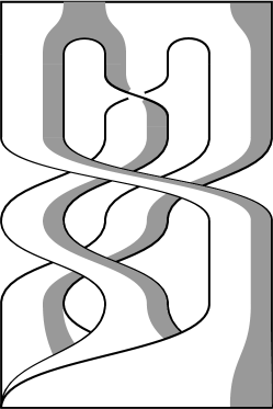
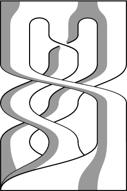
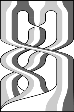
(a) $T_{\mathcal{E}_{1}}\subset T_{\mathcal{C}}$	(b) $T_{\mathcal{E}_{2}}\subset T_{\mathcal{C}}$	(c) $T_{\mathcal{E}_{1}}$ and $T_{\mathcal{E}_{2}}$ coexisting

Figure 10: Coexisting templates $T_{\mathcal{E}_{1}}$ and $T_{\mathcal{E}_{2}}$ are subtemplates of the template of $\mathcal{C}$.

We propose these subtemplates as illustrated Fig. 10. We compute the concatenation of torsions and mixer that appears in these figures. For $T_{\mathcal{E}_{1}}$, we have two parts: one is a mixer and the other is a strip without torsion. These parts permute negatively once in a writhe; it algebraically corresponds to a concatenation of two negative torsions. Thus, the linking matrix of such a subtemplate (Fig. 10a) is

$$\left[\begin{array}[]{C{1.3em}C{1.3em}}\@add@centering&-1\@add@centering\cr-1\@add@centering&-1\@add@centering\end{array}\right\rsem+\left[-2\right]=\left[\begin{array}[]{C{1.3em}C{1.3em}}-2\@add@centering&-3\@add@centering\cr-3\@add@centering&-3\@add@centering\end{array}\right\rsem=T(\mathcal{E}_{1})\;.$$ (15)

Similarly, the linking matrix of $T_{\mathcal{E}_{2}}$ as a subtemplate (Fig. 10b) is

$$\left[\begin{array}[]{C{1.3em}C{1.3em}}-1\@add@centering&-1\@add@centering\cr-1\@add@centering&\@add@centering\end{array}\right\rsem+\left[-2\right]=\left[\begin{array}[]{C{1.3em}C{1.3em}}-3\@add@centering&-3\@add@centering\cr-3\@add@centering&-2\@add@centering\end{array}\right\rsem=T(\mathcal{E}_{2})\;.$$ (16)

These algebraical relations between template and subtemplate linking matrices with Fig. 10 prove that $T_{\mathcal{E}_{1}}\subset T_{\mathcal{C}}$ and $T_{\mathcal{E}_{2}}\subset T_{\mathcal{C}}$. Moreover, these two subtemplates are symmetric one to the other by reflection and coexist in the template of $\mathcal{C}$ (Fig. 10c).

4.2.2 Concatenation of mixers

We now consider $T_{\mathcal{F}}$, the template of $\mathcal{F}$, made of four strips. In a previous paper [15], we demonstrate that the concatenation of two mixers is a mixer and its number of strips is the product of the number of strips of each mixer. Thus, the concatenation of two mixers made of two branches is a mixer with four branches. Our hypothesis is that the four strips of $T_{\mathcal{F}}$ are the result of this process. To validate it, we draw its subtemplate by splitting the template of $\mathcal{C}$ into the two symmetric part containing a mixer; we obtain the Fig. 11a.

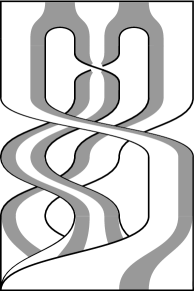
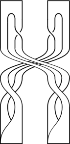
(a) $T_{\mathcal{F}}\subset T_{\mathcal{C}}$	(b) $T_{\mathcal{F}}$

Figure 11: (a) The template of $\mathcal{F}$ is a subtemplate of the template of $\mathcal{C}$. (b) $T_{\mathcal{F}}$ with two mixers.

As we do previously, we decompose this subtemplate (Fig. 11b) in parts: the two parts contain a mixer and these parts permute negatively once. Thus, we concatenate a mixer before a mixer and two negative torsions (cf. 4.2.1). The first concatenation gives a mixer defined by a linking matrix; the algebraical relation necessary to obtain this matrix are detailed in [15]. The linking matrix of $T_{\mathcal{F}}$ as a subtemplate (Fig. 11a) is:

$$\begin{array}[]{l}\left[\begin{matrix}-1&-1\\ -1&0\end{matrix}\right\rsem+\left[\begin{matrix}0&-1\\ -1&-1\end{matrix}\right\rsem+[-2]\\ \quad=\left[\left|\begin{array}[]{C{1.3em}C{1.3em}C{1.3em}C{1.3em}}-1\@add@centering&-1\@add@centering&-1\@add@centering&-1\@add@centering\cr-1\@add@centering&-1\@add@centering&-1\@add@centering&-1\@add@centering\cr-1\@add@centering&-1\@add@centering&\@add@centering&\@add@centering\cr-1\@add@centering&-1\@add@centering&\@add@centering&\@add@centering\end{array}\right|+\left|\begin{array}[]{C{1.3em}C{1.3em}C{1.3em}C{1.3em}}\@add@centering&\@add@centering&\@add@centering&\@add@centering\cr\@add@centering&\@add@centering&\@add@centering&1\@add@centering\cr\@add@centering&\@add@centering&\@add@centering&\@add@centering\cr\@add@centering&1\@add@centering&\@add@centering&\@add@centering\end{array}\right|+\left|\begin{array}[]{C{1.3em}C{1.3em}C{1.3em}C{1.3em}}-1\@add@centering&-1\@add@centering&-1\@add@centering&-1\@add@centering\cr-1\@add@centering&\@add@centering&\@add@centering&-1\@add@centering\cr-1\@add@centering&\@add@centering&\@add@centering&-1\@add@centering\cr-1\@add@centering&-1\@add@centering&-1\@add@centering&-1\@add@centering\end{array}\right|\right\rsem+[-2]\\ \quad=\left[\begin{array}[]{C{1.3em}C{1.3em}C{1.3em}C{1.3em}}-2\@add@centering&-2\@add@centering&-2\@add@centering&-2\@add@centering\cr-2\@add@centering&-1\@add@centering&-1\@add@centering&-1\@add@centering\cr-2\@add@centering&-1\@add@centering&\@add@centering&-1\@add@centering\cr-2\@add@centering&-1\@add@centering&-1\@add@centering&-1\@add@centering\end{array}\right\rsem+[-2]=\left[\begin{array}[]{C{1.3em}C{1.3em}C{1.3em}C{1.3em}}-4\@add@centering&-4\@add@centering&-4\@add@centering&-4\@add@centering\cr-4\@add@centering&-3\@add@centering&-3\@add@centering&-3\@add@centering\cr-4\@add@centering&-3\@add@centering&-2\@add@centering&-3\@add@centering\cr-4\@add@centering&-3\@add@centering&-3\@add@centering&-3\@add@centering\end{array}\right\rsem=T(\mathcal{F})\end{array}$$ (17)

This algebraical relation between template and subtemplate linking matrices associated to Fig. 11 prove that $T_{\mathcal{F}}\subset T_{\mathcal{C}}$.

We now consider the attractor $\mathcal{D}$, we have $T_{\mathcal{D}}\subset T_{\mathcal{F}}$ directly from their mixers

$$\left[\begin{array}[]{C{1.3em}C{1.3em}C{1.3em}}-4\@add@centering&-4\@add@centering&-4\@add@centering\cr-4\@add@centering&-3\@add@centering&-3\@add@centering\cr-4\@add@centering&-3\@add@centering&-2\@add@centering\end{array}\right\rsem\subset\left[\begin{array}[]{C{1.3em}C{1.3em}C{1.3em}C{1.3em}}-4\@add@centering&-4\@add@centering&-4\@add@centering&-4\@add@centering\cr-4\@add@centering&-3\@add@centering&-3\@add@centering&-3\@add@centering\cr-4\@add@centering&-3\@add@centering&-2\@add@centering&-3\@add@centering\cr-4\@add@centering&-3\@add@centering&-3\@add@centering&-3\@add@centering\end{array}\right\rsem\;;$$ (18)

this is illustrated on Fig. 12. We previously obtain that $T_{\mathcal{F}}\subset T_{\mathcal{C}}$, thus we prove that $T_{\mathcal{D}}\subset T_{\mathcal{C}}$.

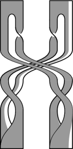
Figure 12: Template of $\mathcal{D}$ is a subtemplate of the template of $\mathcal{F}$ and consequently, it is also a subtemlate of the template of $\mathcal{C}$.

Consequently, we prove that the six templates of attractors $\mathcal{A}$, $\mathcal{B}$, $\mathcal{D}$, $\mathcal{E}_{1}$, $\mathcal{E}_{2}$ and $\mathcal{F}$ are subtemplate of the template of the attractor $\mathcal{C}$; it is a template with six subtemplates. We remind that $\mathcal{G}$ and $\mathcal{C}$ have the same template ($T_{\mathcal{G}}=T_{\mathcal{C}}$).

5 A template for the whole bifurcation diagram

We obtain a unique template containing the eight templates of attractors. We now consider the whole bifurcation diagram (Fig. 1) and not only specific attractors. In this section, we will show that the template of $\mathcal{C}$ contains all attractors templates for any parameter value take from this bifurcation diagram. We use the Poincaré section (3) and build return maps using $y_{n}$ for $\alpha\in]-2;1.8[$ when an attractor is solution. We associate a symbolic dynamic with the three symbols “$0$”, “$1$”, “$2$” of $T_{\mathcal{C}}$. Note that Barrio et al. [20] also use this process to study return maps of a Rössler system from a Lyapunov diagram. The authors display return maps with superstability curve and coexisting stable points. Here we prefer collect extrema points to make a partition of the bifurcation diagram.

Figure 13: Partition of the bifurcation diagram when $\alpha$ varies build using first return maps on $y_{n}$ of the Poincaré section (3). This partition give a symbolic dynamic with three symbols “$0$”, “$1$”, “$2$” depending on $\alpha$.

In the diagram Fig. 13, we indicate the values of $y_{n}$ splitting the return maps into two or three parts. We remind the reader that we orientate application from the inside to the outside of the attractor. Thus, the branches are labelled with symbol number increasing while $y_{n}$ decrease. Fig. 13 reveals that the separator values are linear to $\alpha$. We note $y_{0|1}(\alpha)$ the value of $y_{n}$ that split branches “$0$” and “$1$” and $y_{1|2}(\alpha)$ the value of $y_{n}$ that split branches “$1$” and “$2$”. A linear regression gives

$$\begin{array}[]{l}y_{0|1}(\alpha)=1.43638\alpha-6.76016\\ y_{1|2}(\alpha)=2.18237\alpha-11.1289\;.\end{array}$$ (19)

Up to this point, if there is an attractor solution, its orbits can be encoded with the symbols depending on the previous equations. This also requires the use of the Poincaré section (3).

For a given range of a bifurcation parameters ($\alpha\in]-2;1.8[$), the parameters of the Rössler system depends on $\alpha$: $a(\alpha)$, $b(\alpha)$ and $c(\alpha)$. The fixed points depend on the parameters and the Poincaré section depend on the fixed points. Thus, we obtain a Poincaré section and its partition (19) depending on $\alpha$ while the template is define by the linking matrix

$$\left[\begin{array}[]{C{1.3em}C{1.3em}C{1.3em}}\@add@centering&-1\@add@centering&-1\@add@centering\cr-1\@add@centering&-1\@add@centering&-1\@add@centering\cr-1\@add@centering&-1\@add@centering&\@add@centering\end{array}\right\rsem\;.$$ (20)

The main result is that the topological characterization of chaotic attractors can be extended as a description of various attractors whose parameters come from one bifurcation diagram. In this bifurcation diagram, we show that there are regimes where the chaotic mechanisms are topologically equivalent ($T_{\mathcal{C}}=T_{\mathcal{G}}$), symmetric ($T_{\mathcal{E}_{1}}$ and $T_{\mathcal{E}_{2}}$) and they are a subset of the same chaotic mechanism. The point is that our work can help to understand the complex structure of attractors considering them as subtemplates of their neighbors (in term of bifurcation parameter). This also enlarge the possibility to use the topological characterization to describe more than an attractor, but an entire bifurcation diagram.

6 Conclusion

In this paper we study eight attractors of the Rössler system. The parameters values of these attractors come from a bifurcation diagram that exhibits various dynamics such as coexisting attractors. For each attractor we apply the topological characterization method that give us a template of the attractor. These templates detail the chaotic mechanism and these are only made of stretching and folding mechanism followed by a squeezing mechanism with two, three and four strips.

The second part of this paper is dedicated to the proof that the eights templates are subtemplates of a unique template: the template of $\mathcal{C}$. The main result here is that a template is no longer a tool to describe one attractor but also a set of neighbours attractors (in the parameter space). Thus for a bifurcation diagram, we build a partition using symbols of $T_{\mathcal{C}}$. This partition over the whole diagram give a global structure of attractors for a range of parameters.

This better understanding of the structure of bifurcation diagram can help researchers that want to explore the behaviour of their system, especially if it exhibits chaotic properties. For instance Matthey et al. [21] design a robot using coupled Rössler oscillators to simulate its locomotion. A similar theoretical analysis of their system can provide various set of parameters with specific chaotic properties that might induce new locomotion pattern. A partitioned bifurcation diagram details the various non equivalent dynamical behavior of the system to find them.

This work on templates of attractors from a unique bifurcation diagram is a first step that can lead to a description of manifolds using templates. It is also a new way to classify templates grouping them as subtemplates and not claiming that it exists six new attractors for the Rössler system. To conclude, this work permits to apply the topological characterization method to a set of attractors from a bifurcation diagram. The partition of a bifurcation diagram associated with a unique template is a new tool to describe the global dynamical properties of a system while a parameter is varied. In future works, we will apply this method on attractors bounded by higher genus torus to highlight how symmetry breaking or template number of branches are related in a bifurcation diagram.

References

References

- [1] Rössler O E 1976 An equation for continuous chaos Physics Letters A 57(5) 397-398
- [2] Castro V, Monti M, Pardo W B, Walkenstein J A and Rosa E 2007 Characterization of the Rössler system in parameter space, International Journal of Bifurcation and Chaos 17(3) 965-973
- [3] Barrio R, Blesa F and Serrano S 2009 Qualitative analysis of the Rössler equations: Bifurcations of limit cycles and chaotic attractors Physica D: Nonlinear Phenomena 238(13) 1087-1100
- [4] Genesio R, Innocenti G and Gualdani F 2008 A global qualitative view of bifurcations and dynamics in the Rössler system Physics Letters A 372 1799-1809
- [5] Sprott J C and Li C 2016 Asymmetric bistability in the Rössler system International Journal of Bifurcation and Chaos submitted
- [6] Gilmore R and Lefranc M 2002 The Topology of Chaos NY: Wiley
- [7] Letellier C, Dutertre P and Maheu B 1995 Unstable periodic orbits and templates of the Rössler system: toward a systematic topological characterization Chaos 5(1) 271-282
- [8] Rosalie M and Letellier C 2014 Toward a general procedure for extracting templates from chaotic attractors bounded by high genus torus International Journal of Bifurcation and Chaos 24(4) 1450045
- [9] Birman J and Williams R F 1983 Knotted periodic orbits in dynamical systems -I: Lorenz’s equations Topology 22(1) 47-82
- [10] Franks J and Williams R F 1985 Entropy and knots, Transactions of the American Mathematical Society 921(1) 241-253
- [11] Poincaré H 1899 Les méthodes nouvelles de la mécanique céleste Volume 1-3 Gauthier-Villars Paris
- [12] Ghrist R W, Holmes P J and Sullivan M C, 1997 Knots and links in three-dimensional flows Books, Monographs and Lecture Notes 1
- [13] Gilmore R 1998 Topological analysis of chaotic dynamical systems Reviews of Modern Physics 70(4) 1455
- [14] Rosalie M and Letellier C 2013 Systematic template extraction from chaotic attractors: I-Genus-one attractors with an inversion symmetry Journal of Physics A: Mathematical & Theoretical 46(37) 375101
- [15] Rosalie M and Letellier C 2015 Systematic template extraction from chaotic attractors: II. Genus-one attractors with multiple unimodal folding mechanisms Journal of Physics A: Mathematical & Theoretical 48(23) 235101
- [16] Tsankov T D and Gilmore R 2003 Strange attractors are classified by bounding tori Physical Review Letters 91(13) 134104
- [17] Melvin P and Tufillaro N B 1991 Templates and framed braids, Physical Review A 44(6) 3419-3422
- [18] Le Sceller L, Letellier C and Gouesbet G 1994 Algebraic evaluation of linking numbers of unstable periodic orbits in chaotic attractors Physical Review E 49(5) 4693-4695
- [19] Letellier C, Meunier-Guttin-Cluzel S and Gouesbet G 1999 Topological invariants in period-doubling cascades Journal of Physics A 33 1809-1825
- [20] Barrio R, Blesa F and Serrano S 2012 Topological changes in periodicity Hubs of dissipativity systems, Physical Review Letters 108 214102
- [21] Matthey L, Righetti L and Ijspeert A J 2008 Experimental study of limit cycle and chaotic controllers for the locomotion of centipede robots, Intelligent Robots and Systems, 2008. IROS 2008. IEEE/RSJ International Conference on. IEEE