$\eta_{c}\rightarrow l^{+}l^{-}$ and $\chi_{c0}\rightarrow l^{+}l^{-}$ decays revisited

Abstract

We present a calculation of $\eta_{c}\rightarrow l^{+}l^{-}$ and $\chi_{c0}\rightarrow l^{+}l^{-}$ decay widths. The amplitudes are computed within leading-order approximation using NRQCD framework. Numerical results for the branchings fractions are presented.

Introduction. The leptonic decays of $C$-even charmonia have very small branching fractions because the amplitudes are suppressed by $\alpha^{2}$ with respect to the two photon decay modes. For the (pseudo-)scalars $\eta_{c}$ and $\chi_{c0}$ no experimental determination of an upper limit for the dileptonic branching fractions has been reported. Experimental studies of $\eta_{c}$ and $\chi_{c0}$ decays usually use the mesons produced by radiative transitions of the vector charmonia: $J/\psi$ and $\psi(2S)$, respectively. However, the searches for the dielectron decay modes could instead use formation processes: $e^{+}e^{-}\to\eta_{c}$ and $e^{+}e^{-}\to\chi_{c0}$ where the (pseudo-)scalar meson production is tagged using one of its common decays. This method has an advantage of low background and could provide high sensitivity. The method has been applied e.g. for searches of the $\eta^{\prime}\to e^{+}e^{-}$ process at VEPP-2000 where an impressive upper limit for the branching fraction of $5.6\times 10^{-9}$ at 90% C.L. was achieved using integrated luminosity of $2.9$ pb^-1 [1, 2]. In case of $C$-even charmonia such experiments are possible at BEPC-II collider with the BESIII detector [3].

Calculations of the leptonic decay amplitudes can be carried out using the NRQCD framework, see e.g. Refs.[4, 5, 6]. Recently such calculations have been performed for the $\chi_{c1}$ and $\chi_{c2}$ decays in Ref.[7]. The decays $\eta_{c}\rightarrow l^{+}l^{-}$ and $\chi_{c0}\rightarrow l^{+}l^{-}$ can also be described in the same framework. However, the corresponding amplitudes are suppressed by an additional factor $m_{l}/m_{c}$ where $m_{l}$ and $m_{c}$ are lepton and charm quark masses, respectively. This is a consequence of the conservation of the orbital momentum: the lepton helicity flip is mandatory in decays of (pseudo-)scalar mesons. The dominant diagrams with two photons in the intermediate state are shown in Fig.1.

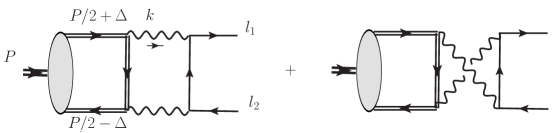
Figure 1: One-loop diagrams describing the annihilation into lepton pair with momenta $l_{1}$ and $l_{2}$.

The gray blob in the figure denotes the charmonium bound state with momentum $P$. In this figure we assume that the dominant contribution is associated with the leading-order $Q\bar{Q}$ component of the wave function. This assumption is valid if the dominant contribution to the corresponding loop integral comes from region(s) with the large virtuality of the intermediate heavy quark $\left(\frac{1}{2}P+\Delta-k\right)^{2}-m^{2}\gg(mv)^{2}$, where $m$ denotes the heavy quark mass and $v$ is the small relative velocity of the heavy quarks. On the other hand the virtualities of the photons and lepton can be arbitrary because these particles belong to the QED sector. For such case the resulting integral yields the leading-order approximation and the overlap with the physical state is described by the matrix element which can be associated with the two quark component of the charmonium wave function. However, as it was shown in Ref.[7] such simple picture is not valid for the $P$-states and resulting interpretation is more complicated. In the following we provide a short description for the decay amplitudes of $\eta_{c}$ and $\chi_{c0}$.

Calculation of the amplitude and branching fraction for $\eta_{c}\rightarrow l^{+}l^{-}$. The decay amplitude reads

$$A_{\eta_{c}\rightarrow ll}\simeq D_{\gamma\gamma}~{}\left\langle 0\right|~{}\psi_{\omega}^{{\dagger}}\gamma_{5}\chi_{\omega}~{}\left|\eta_{c}\right\rangle,$$ (1)

where $\psi_{\omega}^{{\dagger}}$ and$~{}\chi_{\omega}$ denote the heavy quark fields in the heavy quark effective theory (HQET), $\omega$ is the velocity of the heavy meson

$$P=M\omega=l_{1}+l_{2},$$ (2)

$M$ denotes the mass of $\eta_{c}$ and we use the rest frame where $\omega=(1,\vec{0})$. The HQET fields satisfy

$$\psi_{\omega}^{{\dagger}}\hbox to0.0pt{\hbox to6.22453pt{\hfil/\hfil}\hss}\omega=\psi_{\omega}^{{\dagger}},~{}\ \hbox to0.0pt{\hbox to6.22453pt{\hfil/\hfil}\hss}\omega\chi_{\omega}=-\chi_{\omega}.$$ (3)

The matrix element in Eq.(1) reads

$$\left\langle 0\right|~{}\psi_{\omega}^{{\dagger}}\gamma_{5}\chi_{\omega}~{}\left|\eta_{c}\right\rangle=\sqrt{2M}\sqrt{\frac{3}{2\pi}}~{}R_{10}(0),$$ (4)

where $R_{10}(0)$ is the radial component of the charmonium wave function at the origin.

The coefficient $D_{\gamma\gamma}$ in Eq.(1) is given by the diagrams in Fig.1 and reads (Feynman gauge, $e_{c}=2/3$, is used)

$$D_{\gamma\gamma} =-\alpha^{2}e_{c}^{2}\int\frac{d^{4}k}{i\pi^{2}}~{}\bar{u}(l_{1})D_{l}^{\alpha\beta}v(l_{2})\frac{1}{\left[k^{2}-2m(k\omega)\right]}$$

$$~{}\ \ \ \ \ \times~{}\frac{1}{4}\text{Tr}\left[(1+\hbox to0.0pt{\hbox to6.22453pt{\hfil/\hfil}\hss}\omega)\gamma_{5}\gamma^{\beta}(m\hbox to0.0pt{\hbox to6.22453pt{\hfil/\hfil}\hss}\omega-\hbox to0.0pt{\hbox to5.52084pt{\hfil/\hfil}\hss}k+m)\gamma^{\alpha}+\gamma^{\alpha}(\hbox to0.0pt{\hbox to5.52084pt{\hfil/\hfil}\hss}k-m\hbox to0.0pt{\hbox to6.22453pt{\hfil/\hfil}\hss}\omega+m)\gamma^{\beta}\right].$$ (5)

In the above expression the small relative momentum in the heavy quark propagator is neglected

$$\left(\frac{1}{2}P+\Delta-k\right)^{2}-m^{2}\simeq k^{2}-2m(k\omega).$$ (6)

In the numerator of the leptonic part we keep the linear terms in $m_{l}$

$$\bar{u}(l_{1})D_{l}^{\alpha\beta}v(l_{2})\simeq\bar{u}_{n}\left(1+\frac{\hbox to0.0pt{\hbox to5.00002pt{\hfil$\bar{n}$\hfil}\hss}/}{2}\frac{m_{l}}{M}\right)\frac{\gamma^{\alpha}(\hbox to0.0pt{\hbox to5.00002pt{\hfil$l$\hfil}\hss}/_{1}-\hbox to0.0pt{\hbox to5.52084pt{\hfil/\hfil}\hss}k+m_{l})\gamma^{\beta}}{\left[k^{2}\right]\left[\left(k-l_{1}\right)^{2}-m_{l}^{2}\right]\left[\left(k-P\right)^{2}\right]}\left(1-\frac{m_{l}}{M}\frac{\hbox to0.0pt{\hbox to6.00235pt{\hfil/\hfil}\hss}n}{2}\right)v_{\bar{n}}.$$ (7)

The last expression uses auxiliary light cone vectors $n$ and $\bar{n}$ related to the lepton momenta

$$l_{1}=M\frac{n}{2}+\mathcal{O}(1/m),~{}\ \ l_{2}=M\frac{\bar{n}}{2}+\mathcal{O}(1/m).$$ (8)

The spinors in Eq.(7) has been decomposed as

$$\bar{u}(l_{1})\simeq\bar{u}_{n}\left(1+\frac{\hbox to0.0pt{\hbox to5.00002pt{\hfil$\bar{n}$\hfil}\hss}/}{2}\frac{m_{l}}{M}\right),~{}\bar{u}_{n}=\bar{u}(l_{1})\frac{\hbox to0.0pt{\hbox to5.00002pt{\hfil$\bar{n}$\hfil}\hss}/\hbox to0.0pt{\hbox to6.00235pt{\hfil/\hfil}\hss}n}{4},\$$ (9)

$$v(l_{2})\simeq\left(1-\frac{m_{l}}{M}\frac{\hbox to0.0pt{\hbox to6.00235pt{\hfil/\hfil}\hss}n}{2}\right)v_{\bar{n}},~{}\ v_{\bar{n}}=\frac{\hbox to0.0pt{\hbox to5.00002pt{\hfil$\bar{n}$\hfil}\hss}/\hbox to0.0pt{\hbox to6.00235pt{\hfil/\hfil}\hss}n}{4}v(l_{2}).$$ (10)

Using the threshold expansion technique developed in Ref.[5], one finds the following dominant regions: hard $k\sim m$, lepton collinear  $k\sim l_{1}$ or $k\sim l_{2}$ and lepton ultrasoft $k-l_{1}\sim m_{l}$ with $\left(k-l_{1}\right)^{2}-m_{l}^{2}\sim m_{l}^{2}$. In all cases the virtuality of the heavy quark propagator is of order $m^{2}$, i.e. large. We can therefore proceed with the loop calculations neglecting the small momentum components as it is done in Eq.(6). The lepton mass can not be completely neglected because it serves as a natural regulator in the collinear and ultrasoft regions. Therefore the result depends on the large logarithms $\ln m_{l}/m_{c}$. Computing the integral in Eq.(5) we obtain

$$A_{\eta_{c}\rightarrow ll}=\left\langle 0\right|~{}\psi_{\omega}^{{\dagger}}\gamma_{5}\chi_{\omega}~{}\left|\eta_{c}\right\rangle~{}\bar{u}_{n}\gamma_{5}v_{\bar{n}}~{}\alpha^{2}\frac{m_{l}}{M}\frac{e_{c}^{2}}{m^{2}}\left(\frac{1}{4}\ln^{2}\lambda-\ln\lambda+4\ln 2+\frac{\pi^{2}}{12}+\frac{i\pi}{2}\ln\lambda\right),$$ (11)

where

$$\lambda=\frac{m_{l}^{2}}{4m^{2}}.$$ (12)

In order to get the numerical estimate we use $\alpha=1/137$, $m_{c}=1.5$ GeV, $m_{e}=0.51$ MeV, $m_{\mu}=105.6$ MeV and the value of $R_{10}(0)$ from Ref.[8] for Buchmüller-Tye potential [9]:

$$\left|R_{10}(0)\right|^{2}\simeq 0.81~{}\text{GeV}^{3}.$$ (13)

With these parameters we get

$$~{}\ Br\left[\eta_{c}\rightarrow e^{+}e^{-}\right]=5.6\times 10^{-13},\ ~{}Br\left[\eta_{c}\rightarrow\mu^{+}\mu^{-}\right]=1.66\times 10^{-9}.$$ (14)

Alternatively one can consider the branching fractions ratio where $R_{10}(0)$ cancels

$$\frac{Br\left[\eta_{c}\rightarrow e^{+}e^{-}\right]}{Br\left[\eta_{c}\rightarrow\gamma\gamma\right]}=1.6\times 10^{-9},~{}\ \frac{Br\left[\eta_{c}\rightarrow\mu^{+}\mu^{-}\right]}{Br\left[\eta_{c}\rightarrow\gamma\gamma\right]}=4.7\times 10^{-6}.$$ (15)

Using value for $Br\left[\eta_{c}\rightarrow\gamma\gamma\right]=1.57\times 10^{-4}$ [10] we obtain

$$\ Br\left[\eta_{c}\rightarrow e^{+}e^{-}\right]=2.5~{}\times 10^{-13},\ ~{}Br\left[\eta_{c}\rightarrow\mu^{+}\mu^{-}\right]=0.74~{}\times 10^{-9}.$$ (16)

These estimates are about factor two smaller then the values in Eq.(14). The difference can be considered as an estimate of theoretical uncertainty of in this approach.

The $\eta_{c}\rightarrow l^{+}l^{-}$ process has been previously studied in Ref.[11] using a different theoretical approach. Our estimate for $Br\left[\eta_{c}\rightarrow\mu^{+}\mu^{-}\right]$ is in agreement with the one from this reference within the uncertainties, but the results for $Br\left[\eta_{c}\rightarrow e^{+}e^{-}\right]$ differ by factor of six.

Calculation of the amplitude and branching fraction for $\chi_{c0}\rightarrow l^{+}l^{-}$. In this case the the description of the amplitude in the effective theory framework is more complicated. The integral originating from the diagram in Fig.1 has an infrared singularity because there is a region of the integration where the heavy quark propagator becomes soft. Therefore in order to obtain a consistent description in NRQCD one has to include a contribution associated with higher Fock component of the charmonium wave function  $\left|QQ\gamma\right\rangle$. This can be done in the same way as for decay $\chi_{cJ}\rightarrow l^{+}l^{-}$ with $J=1,2$, see e.g. Ref.[7]. In addition one has to take into account the collinear and soft regions which could also be relevant. Therefore the expression for the amplitude can be represented as a sum of two terms

$$A_{\chi_{0}\rightarrow ll}\simeq i\bar{u}_{n}v_{\bar{n}}\frac{m_{l}}{m}~{}\left\{C_{\gamma\gamma}^{(0)}(\mu_{F})\left\langle\mathcal{O}(^{3}P_{0})\right\rangle-\frac{\alpha}{\pi}e_{Q}C_{\gamma}\frac{1}{\sqrt{3}}h(\mu_{F})\right\}.$$ (17)

The first term in Eq.(17) describes the contribution which overlaps with $Q\bar{Q}$ components of the charmonium wave function. In this case

$$\left\langle\mathcal{O}(^{3}P_{0})\right\rangle\equiv\left\langle 0\right|\frac{1}{2\sqrt{3}}~{}\chi_{\omega}^{{\dagger}}\overleftrightarrow{D}_{\top}^{\alpha}\gamma_{\top}^{\alpha}\psi_{\omega}~{}\left|\chi_{c0}\right\rangle=\sqrt{2N_{c}}\sqrt{2M_{\chi_{c0}}}\sqrt{\frac{3}{4\pi}}R_{21}^{\prime}(0),$$ (18)

where $R_{21}^{\prime}(0)$ denotes the derivative of the wave function at the origin. The subscript _⊤ is used for the Lorentz indices which are orthogonal to the velocity $\omega$, for instance, $\omega_{\alpha}\gamma_{\top}^{\alpha}=0$. The hard coefficient function $C_{\gamma\gamma}^{(0)}(\mu_{F})$ is associated with the integration regions where the heavy quark propagator is hard. In this case we find the same dominant regions as described above for the $\eta_{c}$ decay.

However in present case there is an additional domain when the photon momentum is ultrasoft, $k_{\mu}\sim mv^{2}$. The overlap of the hard and the ultrasoft regions leads to the logarithmic divergence that introduces a dependence on the factorization scale $\mu_{F}$. In the ultrasoft region the heavy quark propagator is soft $\left(\frac{1}{2}P+\Delta-k\right)^{2}-m^{2}\sim(mv)^{2}$ and therefore the corresponding contribution cannot be given by the matrix element associated with $Q\bar{Q}$ component of the charmonium wave function. Corresponding contribution is given by the second term on r.h.s. of Eq.(17) where the quantity $h(\mu_{F})$ is defined by the following matrix element

$$\left\langle 0\right|~{}\chi_{\omega}^{{\dagger}}\gamma_{\top}^{\sigma}\psi_{\omega}Y_{n}^{{\dagger}}Y_{\bar{n}}~{}\left|\chi_{c0}\right\rangle=-\frac{1}{2}(n-\bar{n})^{\sigma}~{}i\frac{\alpha}{\pi}e_{Q}\frac{1}{\sqrt{3}}h(\mu_{F}),$$ (19)

with the ultrasoft photon Wilson lines

$$Y_{n}^{{\dagger}}=\text{Pexp}\left\{ie\int_{0}^{\infty}ds~{}n\cdot B^{us}(sn)\right\},~{}\ Y_{\bar{n}}=\text{\={P}exp}\left\{-ie\int_{0}^{\infty}ds~{}\bar{n}\cdot B^{us}(s\bar{n})\right\},~{}\$$ (20)

where $B_{\mu}^{us}$ denotes the ultrasoft photon field. In the leading-order approximation with respect to the electromagnetic coupling $e$ these Wilson lines are equal to unity $Y_{n}^{{\dagger}}=Y_{\bar{n}}=1+\mathcal{O}(e)$. Then the matrix element in Eq.(19) vanishes because of $C$-parity. One has to pick up at least one term $\sim eB^{us}$ in the expansion of the Wilson lines in order to get the $C$-even operator. Therefore we can conclude that the matrix element in Eq.(19) can be associated with the coupling to the higher Fock component $\left|Q\bar{Q}\gamma\right\rangle$ of the charmonium wave function. The value of the corresponding constant $h(\mu_{F})$ in Eq.(19) is the same for all states $\chi_{cJ}$ due to the heavy quark spin symmetry. At low normalization point $\mu_{F}=\mu_{0}\simeq 400$ MeV it can be computed in the low energy effective theory describing interaction of the ultrasoft photons with heavy mesons. The ultasoft matrix element in Eq.(19) also contributes to the decays $\chi_{c1,1}\rightarrow e^{+}e^{-}$ and has been already computed in Ref.[7]

$$h(\mu_{0}) =f_{\gamma}\sqrt{2M_{J/\psi}}\sqrt{\frac{3}{2\pi}}R_{10}(0)\frac{~{}\Delta}{M}\left(1-\ln 2+\ln[\mu_{0}/\Delta]+i\pi\right)$$ (21)

$$+f_{\gamma}^{\prime}\sqrt{2M_{\psi^{\prime}}}\sqrt{\frac{3}{2\pi}}R_{20}(0)\frac{\Delta^{\prime}}{M_{\chi_{0}}}\left(1-\ln 2+\ln[\mu_{0}/|\Delta^{{}^{\prime}}|]\right),$$ (22)

where $\Delta=(M_{\chi_{0}}^{2}-M_{J/\psi}^{2})/2M$, $\Delta^{\prime}=(M_{\chi_{0}}^{2}-M_{\psi^{\prime}}^{2})/2M_{\chi_{0}}$,$~{}R_{10}(0)$ and$~{}R_{20}(0)$ denote the radial wave functions of $J/\psi$ and $\psi^{\prime}$ mesons, respectively. In what follows we take their values from Ref.[8] for Buchmüller-Tye potential. The dimensionless couplings $f_{\gamma}$ and $f_{\gamma}^{\prime}$ can be determined from the decays $\chi_{cJ}\rightarrow J/\psi+\gamma$ and $\psi^{\prime}\rightarrow\chi_{cJ}+\gamma$, respectively

$$f_{\gamma}\simeq 6.0,~{}\ f_{\gamma}^{\prime}\simeq-7.2.$$ (23)

The hard coefficient $C_{\gamma}$ in Eq.(17) is given by the tree diagram describing annihilation subprocess $c\bar{c}\rightarrow e^{+}e^{-}$ and reads

$$C_{\gamma}=\frac{\alpha\pi}{m^{2}}e_{c}.$$ (24)

The determination of the second hard coefficient $C_{\gamma\gamma}^{(0)}$ in Eq.(17) requires calculation of the diagrams in Fig.1 and one-loop calculation of the matrix element in Eq.(19) in the potential NRQED [12, 13, 14]. These calculations are similar to the ones carried out in Ref.[7]. The only difference is that a minimal dependence on the lepton mass $m_{l}$ has to be included in order to avoid IR-singularities in the QED sector. The final result reads

$$C_{\gamma\gamma}^{(0)}(\mu_{F})=\frac{\alpha^{2}}{\sqrt{3}}\frac{e_{c}^{2}}{m^{3}}\left\{2\ln\frac{m^{2}}{\mu_{F}^{2}}+\frac{3}{4}\ln^{2}\lambda+\ln\lambda+\frac{\pi^{2}}{4}+2+6\ln 2+i\pi\left(2\ln 2-1+\frac{3}{2}\ln\lambda\right)\right\},$$ (25)

where $\lambda$ is defined in Eq.(12). The numerical estimates of the branching fractions are

$$Br[\chi_{c0}\rightarrow e^{-}e^{+}]=1.0\times 10^{-12},~{}\ Br[\chi_{c0}\rightarrow\mu^{-}\mu^{+}]=2.2\times 10^{-9}.$$ (26)

We observe that the hard contribution with $C_{\gamma\gamma}^{(0)}$ dominates and practically saturates the numerical values contrary to $\chi_{c1,2}\rightarrow l^{+}l^{-}$ decays where the ultrasoft contribution is the most important, see Ref.[7]. This is explained by a relative enhancement of $C_{\gamma\gamma}^{(0)}$ in Eq.(25) by the large logarithms $\ln\lambda$ with respect to the ultrasoft term $h$ in Eq.(17) which remains unchanged.

The amplitude of the decay $\chi_{cJ}\rightarrow l^{+}l^{-}$ has also been considered in Ref.[15] where only the hard contribution with $C_{\gamma\gamma}^{(0)}$ has been taken into account. The result in Eq.(25) differs from the one in Ref.[15] only by simple non-logarithmic terms. We observe that this discrepancy does not provide any tangible numerical effect. The estimate for $Br[\chi_{c0}\rightarrow l^{+}l^{-}]$ obtained in this work is about factor three larger which is explained by the different choice of the numerical values used for $m_{c}$ and $R^{\prime}_{21}(0)$.

References

[1]
R. R. Akhmetshin et al. [CMD-3 Collaboration],
Phys. Lett. B 740 (2015) 273
doi:10.1016/j.physletb.2014.11.056
[arXiv:1409.1664 [hep-ex]].
[2]
M. N. Achasov et al.,
Phys. Rev. D 91 (2015) 092010
doi:10.1103/PhysRevD.91.092010
[arXiv:1504.01245 [hep-ex]].
[3]
D. M. Asner et al.,
Int. J. Mod. Phys. A 24 (2009) S1
[arXiv:0809.1869 [hep-ex]].
[4]G. T. Bodwin, E. Braaten and G. P. Lepage,
Phys. Rev. D 51 (1995) 1125 [Phys. Rev. D 55 (1997)
5853] [hep-ph/9407339].
[5]M. Beneke and V. A. Smirnov,
Nucl. Phys. B 522 (1998) 321 [hep-ph/9711391].
[6]N. Brambilla, A. Pineda, J. Soto and A. Vairo,
Rev. Mod. Phys. 77 (2005) 1423 [hep-ph/0410047].
[7]
N. Kivel and M. Vanderhaeghen,
JHEP 1602 (2016) 032
doi:10.1007/JHEP02(2016)032
[arXiv:1509.07375 [hep-ph]].
[8] E. J. Eichten and C. Quigg,
Phys. Rev. D 52 (1995) 1726 [hep-ph/9503356].
[9]
W. Buchmuller and S. H. H. Tye,
Phys. Rev. D 24 (1981) 132.
[10]
K. A. Olive et al. [Particle Data Group Collaboration],
Chin. Phys. C 38 (2014) 090001.
[11]
M. Z. Yang,
Phys. Rev. D 79 (2009) 074026
doi:10.1103/PhysRevD.79.074026
[arXiv:0902.1295 [hep-ph]].
[12]A. Pineda and J. Soto,
Nucl. Phys. Proc. Suppl. 64 (1998) 428 [hep-ph/9707481].
[13]
N. Brambilla, A. Pineda, J. Soto and A. Vairo,
Phys. Rev. D 60 (1999) 091502
[hep-ph/9903355].
[14]
N. Brambilla, A. Pineda, J. Soto and A. Vairo,
Nucl. Phys. B 566 (2000) 275
[hep-ph/9907240].
[15]D. Yang and S. Zhao,
Eur. Phys. J. C 72 (2012) 1996 [arXiv:1203.3389 [hep-ph]].