The Simulation of Non-Abelian Statistics of Majorana Fermions in Ising Chain with Z2 Symmetry

Abstract

In this paper, we numerically study the non-Abelian statistics of the zero-energy Majorana fermions on the end of Majorana chain and show its application to quantum computing by mapping it to a spin model with special symmetry. In particular, by using transverse-field Ising model with Z2 symmetry, we verify the nontrivial non-Abelian statistics of Majorana fermions. Numerical evidence and comparison in both Majorana-representation and spin-representation are presented. The degenerate ground states of a symmetry protected spin chain therefore previde a promising platform for topological quantum computation.

I Introduction

Majorana fermions have recently attracted much attention due to the potential application in topological quantum computation ref1 . Majorana fermions are particles that are their own antiparticles — in contrast with the case for Dirac fermions — and obey non-Abelian statisticsref1.1 ; ref1.2 ; ref1.3 . The exotic properties of Majorana fermions have attracted increasing interest from researchersref1.4 ; ref1.5 ; ref1.6 ; ref1.7 ; ref1.9 ; ref1.10 . Majorana fermions with zero energy (Majorana zero modes) had been predicted to be induced by vortices in two-dimensional spinless $p_{x}+ip_{y}$-wave superconductorref2 ; ref3 ; ref4 , or localize at the ends in a one-dimensional spin-polarized superconductor chain. Another creative proposal is the interface of $s$-wave superconductors and topological insulators owing to the proximity effect. On the other hand, the spin chain has been studied in depth both theoretically and experimentally. It is known that the transverse-field Ising model with Z2 symmetry is equivalent to the one-dimensional spin-polarized superconductor modelref5 .

In this paper, we numerically study the non-Abelian statistics of the zero-energy Majorana fermions on the end of Majorana chain and show its application to quantum computing by mapping it to a spin model with special symmetry. In particular, by using transverse-field Ising model with Z2 symmetry, we verify the nontrivial quantum statistics of Majorana fermions numerically using a T-junction wire network, where the Majorana fermions can be braided by tuning local gates. We may also mimic this T-type braiding in spin representation numerically, where the two zero-energy Majorana fermion states correspond to two degenerate ground states of spin chain. In this way, we provide an easy way of detecting the fundamental non-Abelian statistics of Majorana fermions, which is useful to quantum computation.

II Majorana zero modes in one-dimensional quantum spin model with Z2 symmetry

It has been recognized that a one-dimensional quantum spin model with Z2 symmetry is equivalent to a one-dimensional superconductor via Jordan-Wigner transformation. Therefore, we can describe a one-dimensional spin chain using either spin representation ($\sigma$-representation) or fermion representation ($\gamma$-representation). Thus, the Majorana fermion and its statistic property can be represented in either representation.

Here, we start from the one-dimensional Ising chain with Z2 symmetry. The Hamiltonian of the Ising spin chain is given by

$$\hat{H}=\sum_{n=1}^{N-1}J_{n,n+1}\sigma_{n}^{x}\sigma_{n+1}^{x}-\sum_{n=1}^{N}\mu_{n}\vec{\sigma}_{n}$$ (1)

where $J_{n,n+1}$ ( $J_{n,n+1}<0$ ) is the Ising coupling constant between two nearest-neighbour (NN) sites $n,$ $n+1$, $\mu_{n}$ ( $\mu_{n}>0$ ) is the strength of external field on site $n$, and $N$ is the total lattice number of the Ising chain. We then introduce the spin operators $\sigma_{n}^{+},$ $\sigma_{n}^{-}$, $\sigma_{n}^{x}=\sigma_{n}^{+}+\sigma_{n}^{-},$ and $\sigma_{n}^{y}=i(\sigma_{n}^{+}-\sigma_{n}^{-})$. The Z2 symmetry is charaterized by as spin rotation symmetry $\hat{R}=e^{i\pi\sum_{n=1}^{N}\sigma_{n}^{z}}$, i.e.,

$$\hat{R}\hat{H}\hat{R}^{-1}=\hat{H}.$$

Thus, to guarantee the Z2 symmetry, the external field should be along $z$-direction, or $\vec{\sigma}_{n}\rightarrow\sigma_{n}^{z}$.

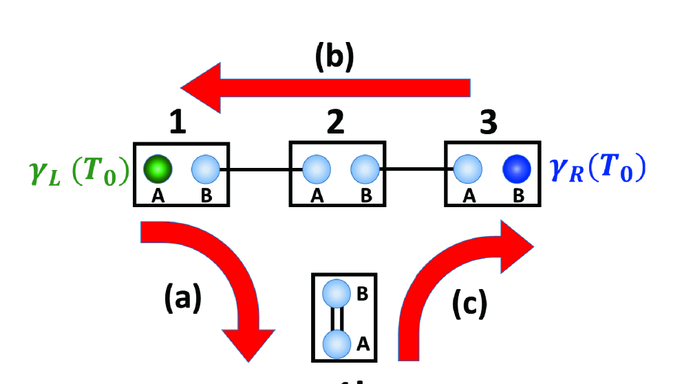
Figure 1: (Color online) Braiding two Majorana fermions.  The braiding process of Majorana fermions is denoted by thick red arrows. For a T-junction, there is one spin in each box $1,2,3,$ and $1^{\prime}$. At the beginning of the braiding two unpaired Majorana fermions locate at the left end $\gamma_{L}(T_{0})$ (green ball) and right end $\gamma_{R}(T_{0})$ (blue ball) of the Majorana chain. We can adiabatically turn on $\mu_{1}$ $(0\rightarrow\mu_{0})$ and turn off $J_{1B,2A}$ $(J_{0}\rightarrow 0)$ drives the left-end Majorana zero mode from site $1A$ to site $2A$. As the same, we drive the two fermions as follow: (a) During $T_{0}$ to $T_{2}$ the most left fermion is driven to the bottom site of box $1^{\prime}$; (b)During $T_{3}$ to $T_{5}$ the most right fermion is driven to the most left site; (c) During $T_{6}$ to $T_{7}$ the bottom one is driven to the most right site. Now the final Majorana modes are denoted by $\gamma_{L}(T_{7})$, $\gamma_{R}(T_{7})$.

The Jordan-Wigner transformation is described byref5 ; ref6

$$\sigma_{n}^{+} =a_{n}^{+}{\displaystyle\prod\limits_{m=1}^{n-1}}a_{l}^{+}a_{l};$$

$$\sigma_{n}^{-} =a_{n}{\displaystyle\prod\limits_{m=1}^{n-1}}a_{l}^{+}a_{l};$$ (2)

$$\sigma_{n}^{z} =2a_{n}^{+}a_{n}-1,$$

where $a_{n}^{+},$ $a_{n}$ denote the creation and annihilation operators of Dirac fermions and obey the anticommutation relation $\left\{a_{m},a_{n}^{+}\right\}=\delta_{m,n}$. By using Jordan-Wigner transformation, the Hamiltonian $\hat{H}$ can be written as

$$\hat{H}=\sum_{n=1}^{N-1}J_{n,n+1}(a_{n}-a_{n}^{+})(a_{n+1}+a_{n+1}^{+})-\sum_{n=1}^{N}\mu_{n}(2a_{n}^{+}a_{n}-1).$$ (3)

Then, the Majorana fermion is defined as

$$\gamma_{n}^{A}=a_{n}^{+}+a_{n},\text{ }\gamma_{n}^{B}=i(a_{n}^{+}-a_{n}),$$ (4)

with $\gamma_{n}^{{\dagger}}=\gamma_{n},$ $\left\{\gamma_{n}^{l},\gamma_{m}^{l^{\prime}}\right\}=2\delta_{m,n}\delta_{l,l^{\prime}}$. From the definition, one can see that Majorana fermions are their own antiparticle and constitute “half” of an ordinary fermion. We obtain the Hamiltonian in the $\gamma$-representation ref20 ,

$$\hat{H}=-i\sum_{n=1}^{N-1}J_{n,n+1}\gamma_{n}^{B}\gamma_{n+1}^{A}-i\sum_{n=1}^{N}\mu_{n}\gamma_{n}^{A}\gamma_{n}^{B}.$$ (5)

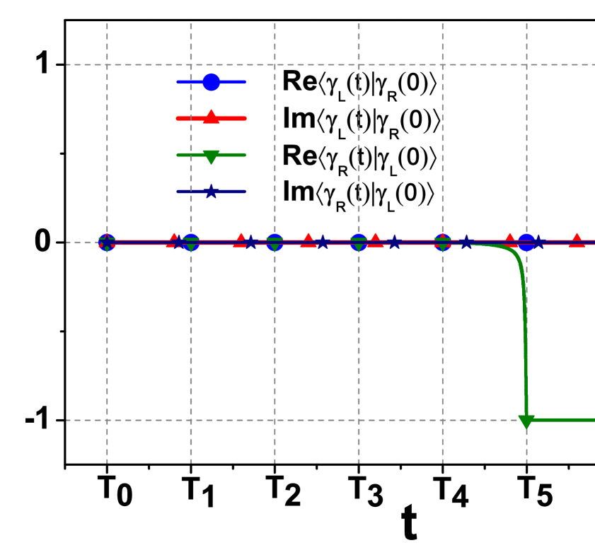
Figure 2: Evolution of particle distribution of Majorana modes during the braiding: $\left|\gamma_{L}(t)\right\rangle$ ($\left|\gamma_{R}(t)\right\rangle$) is the wave function of Majorana zero modes during the braiding at time $t$, which localizes in left (right) end of horizontal chain at time $t=T_{0}=0$. To guarantee the adiabatic condition, i.e. the process is very slow, we set $T_{7}-T_{0}=10000\hbar/J,$ $N_{0}=10^{6}$. After the braiding process, we have $\left\langle\gamma_{L}(T_{7})|\gamma_{L}(0)\right\rangle=\left\langle\gamma_{R}(T_{7})|\gamma_{R}(0)\right\rangle=0,$ $\left|\gamma_{L}(T_{7})\right\rangle=\left|\gamma_{R}(0)\right\rangle,$ $\left|\gamma_{R}(T_{7})\right\rangle=-\left|\gamma_{L}(0)\right\rangle.$ That is $\gamma_{1}^{A}$ $\rightarrow$ $\gamma_{3}^{B}$ and $\gamma_{3}^{B}$ $\rightarrow$ $-\gamma_{1}^{A}.$

In the fermion representation for the Hamiltonian, we see that two Majorana fermions on one site $n$ are coupled and the coupling constant is $\mu_{n}$ (e.g., the double dark line links site A and site B inner the box $1^{\prime}$ in Fig.1) and the two Majorana fermions on the NN sites are linked by $J_{n,n+1}$ (e.g., the single dark line between boxes 1, 2 and 3 in Fig.1). When we adiabatically turn off $\mu_{n}$ at all sites such that its value decreases from a certain value $\mu_{0}$ to zero ($\mu_{0}\rightarrow 0$), the Majorana fermions of the chain are only coupled by $J_{n,n+1}$ terms except for the two Majorana fermions at the ends (e.g., the green and blue balls in Fig.1).

To characterize the quantum states of Majorana fermions, we introduce the creation and annihilation operators of Dirac fermions, $d_{n}=(\gamma_{n+1}^{A}+i\gamma_{n}^{B})/2$, $d_{n}^{{\dagger}}=(\gamma_{n+1}^{A}-i\gamma_{n}^{B})/2$. The operators of Dirac fermions are combined by two Majorana fermions at NN sites, i.e., $n$ and $n+1$. Thus, the Majorana fermions at the left (right) end of the chain $\gamma_{1}^{A}$ $(\gamma_{N}^{B})$ remain unpaired and have zero energyref8 ; ref9 . Here, we focus on the edge fermion and have

$$d_{end}=\frac{1}{2}(\gamma_{1}^{A}+i\gamma_{N}^{B}),\text{ }d_{end}^{{\dagger}}=\frac{1}{2}(\gamma_{1}^{A}-i\gamma_{N}^{B}).$$ (6)

It is obvious that the edge fermion has zero energy. We now define $\left|F\right\rangle$ to be a many-body quantum state with occupied single particle states for $E<0$ and empty single particle states $E\geq 0$. We therefore introduce a Majorana qubit that consists of two basis states $\left|0\right\rangle,$ $\left|1\right\rangle$ defined asref6.1

$$\left|0\right\rangle\equiv d_{end}\left|F\right\rangle,\text{ }\left|1\right\rangle\equiv d_{end}^{{\dagger}}\left|0\right\rangle.$$ (7)

III Numerical verifying non-Abelian statistics of Majorana fermions in $\gamma$-representation

In this part, we numerically study the quantum statistic of the Majorana fermions located at the end of spin chain by using one-dimensional quantum Ising model with Z2 symmetry. To explore the quantum statistic of the Majorana fermions, we take a 4-spin (i.e., 8-$\gamma$) system as an example and braid the Majorana fermions $\gamma_{1}^{A},$ $\gamma_{3}^{B}$ by seven steps using the T-type structure (see the illustration in Fig.1), which is similar to the semiconducting wire networks in Ref.ref11 .

The parameters $J_{n,n+1}$ and $\mu_{n}$ in the original Hamiltonian are given by $J_{nB,(n+1)A}=J_{0}$ and $\mu_{n}=\mu_{0}$, respectively. We first choose the initial state with $J_{nB,(n+1)A}=0$ and $\mu_{n}=0$. Thus, there must exit two unpaired Majorana zero modes located at the left end $\left|\gamma_{L}(T_{0})\right\rangle=\left|\gamma_{1}^{A}\right\rangle$ (green ball) and right end $\left|\gamma_{R}(T_{0})\right\rangle=\left|\gamma_{3}^{B}\right\rangle$ (blue ball) of the Majorana chain. Here $T_{0}=0$ represents the initial time and $T_{n}$ for $n$-th step of braiding process. We denote the quantum states of Majorana modes by $\left|\gamma_{L}(T_{n})\right\rangle,$ $\left|\gamma_{R}(T_{n})\right\rangle,$ $n\in(1,7)$. The Hamiltonian of the system at $T_{0}$ is given by

$$H_{\gamma,T_{0}}=-iJ_{0}\gamma_{1}^{B}\gamma_{2}^{A}-iJ_{0}\gamma_{2}^{B}\gamma_{3}^{A}-i\mu_{0}\gamma_{1^{\prime}}^{A}\gamma_{1^{\prime}}^{B}.$$ (8)

We then do the braiding process step by step (see Fig.1): (a) $\mu_{1}|_{{}_{{}^{T_{0}}}}^{{}_{{}_{{}_{T_{1}}}}}(0\rightarrow\mu_{0})$, $J_{1B,2A}|_{{}_{{}^{T_{0}}}}^{{}_{{}_{{}_{T_{1}}}}}(J_{0}\rightarrow 0)$ (This means we adiabatically turn on $\mu_{1}$ and turn off $J_{1B,2A}$ simultaneously during the time period $t\in(T_{0},$ $T_{1})$), then $\mu_{1^{\prime}}|_{{}_{{}^{T_{1}}}}^{{}_{{}_{{}_{T_{2}}}}}(\mu_{0}\rightarrow 0)$, $J_{1^{\prime}B,2A}|_{{}_{{}^{T_{1}}}}^{{}_{{}_{{}_{T_{2}}}}}(0\rightarrow J_{0})$. The order of this braiding process is $1A\rightarrow 2A\rightarrow 1^{\prime}A;$ (b) $\mu_{3}|_{{}_{{}^{T_{2}}}}^{{}_{{}_{{}_{T_{3}}}}}(0\rightarrow\mu_{0})$, $J_{2B,3A}|_{{}_{{}^{T_{2}}}}^{{}_{{}_{{}_{T_{3}}}}}(J_{0}\rightarrow 0)$, then $J_{1^{\prime}B,2A}|_{{}_{{}^{T_{3}}}}^{{}_{{}_{{}_{T_{4}}}}}(J_{0}\rightarrow 0)$, $J_{1^{\prime}B,2B}|_{{}_{{}^{T_{3}}}}^{{}_{{}_{{}_{T_{4}}}}}(0\rightarrow J_{0})$, next, $\mu_{1}|_{{}_{{}^{T_{4}}}}^{{}_{{}_{{}_{T_{5}}}}}(\mu_{0}\rightarrow 0)$, $J_{1B,2A}|_{{}_{{}^{T_{4}}}}^{{}_{{}_{{}_{T_{5}}}}}(0\rightarrow J_{0})$. The braiding order is $3B\rightarrow 2B\rightarrow 2A\rightarrow 1A$; (c) $\mu_{1^{\prime}}|_{{}_{{}^{T_{5}}}}^{{}_{{}_{{}_{T_{6}}}}}(0\rightarrow\mu_{0})$, $J_{1^{\prime}B,2B}|_{{}_{{}^{T_{5}}}}^{{}_{{}_{{}_{T_{6}}}}}(J_{0}\rightarrow 0)$, then $\mu_{3}|_{{}_{{}^{T_{6}}}}^{{}_{{}_{{}_{T_{7}}}}}(\mu_{0}\rightarrow 0)$, $J_{2B,3A}|_{{}_{{}^{T_{6}}}}^{{}_{{}_{{}_{T_{7}}}}}(0\rightarrow J_{0})$. The braiding order is $1^{\prime}A\rightarrow 2B\rightarrow 3B$.

In particular, during the time period $t\in(T_{3},$ $T_{4})$, we have

$$H_{\gamma,T_{3}} =-iJ_{0}\gamma_{1^{\prime}}^{B}\gamma_{2}^{A}-i\mu_{0}\gamma_{1}^{A}\gamma_{1}^{B}-i\mu_{0}\gamma_{3}^{A}\gamma_{3}^{B},$$ (9)

$$H_{\gamma,T_{4}} =-iJ_{0}\gamma_{1^{\prime}}^{B}\gamma_{2}^{B}-i\mu_{0}\gamma_{1}^{A}\gamma_{1}^{B}-i\mu_{0}\gamma_{3}^{A}\gamma_{3}^{B}.$$ (10)

The operation during this period shifts the Majorana mode from site $2B$ to $2A$ which are on the same box $2$.

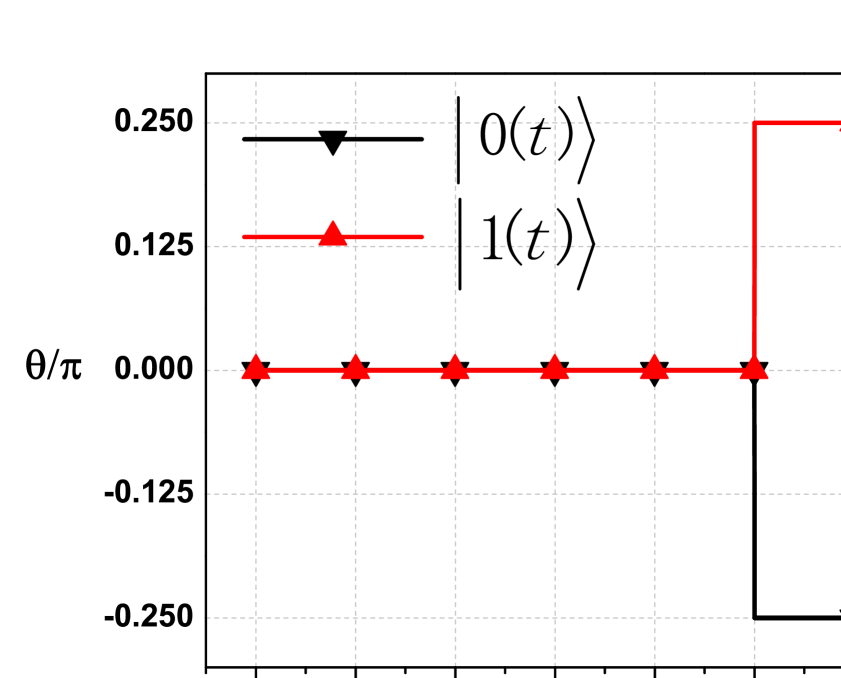
Figure 3: Berry phase during the braiding process: $\left|0(t)\right\rangle$ ($\left|1(t)\right\rangle$) represents one of the two degenerate ground states in spin system, in which spin direction is along $\mathbf{x}$-direction (-$\mathbf{x}$) at the time $t=T_{0}=0$ except for the spin-$1^{\prime}$. The Berry phase of the ground state sharply changes at $t=T_{5}$ where spin-$1$ and spin-$2$ switch from to $\mathbf{x}$-direction to $\mathbf{y}$-direction. As a result, Berry phase changes $\frac{\pi}{4}$ during the braiding process.

It is well known that the braiding of Majorana modes changes not only the amplitude but also the phase of the modes. We next focus on the phase difference of $\left|\gamma_{L}(T_{n})\right\rangle,$ $\left|\gamma_{R}(T_{n})\right\rangle$ before and after the adiabatic braiding process numerically. We diagonalize the initial Hamiltonian $H_{\gamma,T_{0}}$ in the $\gamma$-representation and obtain two zero energy modes $\left|\gamma_{L}(T_{0})\right\rangle=\left|\gamma_{1}^{A}\right\rangle$ and $\left|\gamma_{R}(T_{0})\right\rangle=\left|\gamma_{3}^{B}\right\rangle$. We then define a time-evolution operator

$$U(t)=\hat{T}\left\{\exp[-i\int_{0}^{t}H(t^{\prime})dt^{\prime}]\right\},$$ (11)

where $\hat{T}$ is the time ordering operator. Therefore, at the end of the evolution, we have

$$\left|\gamma_{L}(T_{7})\right\rangle= U(T_{7})\left|\gamma_{L}(T_{0})\right\rangle$$

$$\text{ \ }\left|\gamma_{R}(T_{7})\right\rangle= U(T_{7})\left|\gamma_{R}(T_{0})\right\rangle.$$ (12)

To realize the time-evolution numerically, one may discretize the time-evolution operator employing the times slicing procedure

$$U(T_{7})\approx\hat{T}\vskip 12.0pt plus 4.0pt minus 4.0pt{\displaystyle\prod\limits_{i=0}^{N_{0}}}\exp[-iH(t_{i})\triangle t],\text{ \ }\triangle t=\frac{T_{7}-T_{0}}{N_{0}},$$ (13)

with $\triangle t\ll\hbar/J,$ and $T_{7}-T_{0}$ being sufficiently large. We point out that it is crucial to retain the unitarity throughout the calculation

$$\exp[-iH(t_{i})\triangle t]=A\exp(-i\Lambda\triangle t)A^{{\dagger}},$$ (14)

where $H(t_{i})=A\Lambda A^{{\dagger}},$ $A$ is a unitary matrix $AA^{{\dagger}}=I$ and $\Lambda$ is a diagonal matrix. Fig.2 shows the change in $\left|\gamma_{L}(t)\right\rangle,$ $\left|\gamma_{R}(t)\right\rangle$ during the braiding process. It is clearly that $\left|\gamma_{L}(T_{7})\right\rangle=\left|\gamma_{R}(0)\right\rangle,$ $\left|\gamma_{R}(T_{7})\right\rangle=-\left|\gamma_{L}(0)\right\rangle$. The braiding operation therefore transforms $\gamma_{1}^{A}$ to $\gamma_{3}^{B}$ and $\gamma_{3}^{B}$ to $-\gamma_{1}^{A}$.

IV Numerical verifying non-Abelian statistics of Majorana fermions in $\sigma$-representation

In last section, we have verified the non-Abelian statistics numerically in $\gamma$-representation and construct a phase gate based on the qubits that is simple and easily understoodref11 . We then map the braiding in $\gamma$-representation to that in $\sigma$-representation by employing the Jordan-Wigner transformation ref13 ,

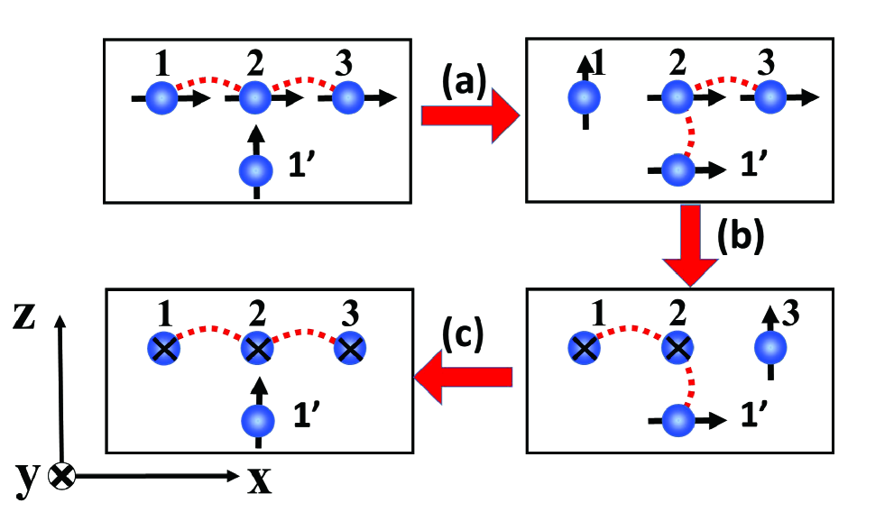
Figure 4: The illustration of braiding Majorana fermions in spin representation: The first picture is an illustration of one of the two degenerate ground states in the spin system which are equal to the two Majorana zero modes in the $\gamma$-representation. Tuning the parameters using the same processes as in Fig.1(a)-(c).

$$\gamma_{n}^{A}=({\displaystyle\prod\limits_{m=1}^{n-1}}\sigma_{m}^{z})\sigma_{n}^{x},\text{ \ \ }\gamma_{n}^{B}=i({\displaystyle\prod\limits_{m=1}^{n}}\sigma_{m}^{z})\sigma_{n}^{x}.$$ (15)

It is obvious that the Majorana fermions $\gamma_{n}^{A}$ and $\gamma_{n}^{B}$ are non-local in the $\sigma$-representation. When $J_{0}<0$ the state $\left|F\right\rangle$ can be written as

$$\left|F\right\rangle=\left|\rightarrow\rightarrow\rightarrow\right\rangle,$$ (16)

where

$$\left|\rightarrow\right\rangle=\frac{\sqrt{2}}{2}\left(\begin{array}[]{c}1\\ 1\end{array}\right),\text{ \ }\left|\leftarrow\right\rangle=\frac{\sqrt{2}}{2}\left(\begin{array}[]{c}1\\ -1\end{array}\right).$$ (17)

Then the two basis states $\left|0\right\rangle$, $\left|1\right\rangle$ of Majorana qubit are represented in $\sigma$-representation as

$$\left|0\right\rangle =\frac{1}{2}(\gamma_{1}^{A}+i\gamma_{3}^{B})\left|F\right\rangle$$

$$=\frac{1}{2}(\sigma_{1}^{x}+i(i{\displaystyle\prod\limits_{m=1}^{3}}\sigma_{m}^{z})\sigma_{3}^{x})\left|F\right\rangle$$ (18)

$$=\frac{\sqrt{2}}{2}(\left|\rightarrow\rightarrow\rightarrow\right\rangle-\left|\leftarrow\leftarrow\leftarrow\right\rangle),$$

$$\left|1\right\rangle =\frac{1}{2}(\gamma_{1}^{A}-i\gamma_{N}^{B})\left|0\right\rangle$$

$$=\frac{1}{2}(\sigma_{1}^{x}-i(i{\displaystyle\prod\limits_{m=1}^{3}}\sigma_{m}^{z})\sigma_{3}^{x})\left|0\right\rangle$$ (19)

$$=\frac{\sqrt{2}}{2}(\left|\rightarrow\rightarrow\rightarrow\right\rangle+\left|\leftarrow\leftarrow\leftarrow\right\rangle).$$

Thus, the two quantum states of Majorana fermions correspond to two degenerate ground states of 1D transverse Ising model with Z2 symmetry.

	$\gamma$-representation	$\sigma$-representation
Fermion operator	$\gamma_{n}^{A},\gamma_{n}^{B}$	$(\prod\limits_{m=1}^{n-1}\sigma_{m}^{z})\sigma_{n}^{x},i(\prod\limits_{m=1}^{n}\sigma_{m}^{z})\sigma_{n}^{x}$
String operator	$i\prod\limits_{m=1}^{N}\gamma_{m}^{A}\gamma_{m}^{B}$	$\prod\limits_{m=1}^{N}\sigma_{m}^{z}$
Basis	$\frac{1}{2}(\gamma_{1}^{A}+i\gamma_{N}^{B})\left|F\right\rangle$	$\frac{\sqrt{2}}{2}(\left|\rightarrow\rightarrow\cdot\rightarrow\right\rangle-\left|\leftarrow\leftarrow\cdot\leftarrow\right\rangle)$
state	$\frac{1}{2}(\gamma_{1}^{A}-i\gamma_{N}^{B})\left|0\right\rangle$	$\frac{\sqrt{2}}{2}(\left|\rightarrow\rightarrow\cdot\rightarrow\right\rangle+\left|\leftarrow\leftarrow\cdot\leftarrow\right\rangle)$
Braiding	Majorana modes	Spin rotation $\pi/2$
process	exchange	around z-axis
Braiding	$\gamma_{1}^{A}\rightarrow\gamma_{N}^{B}$	$\left|0\right\rangle_{\sigma}\rightarrow e^{i\pi/2}\left|0\right\rangle_{\sigma}$
results	$\gamma_{N}^{B}\rightarrow-\gamma_{1}^{A}$	$\left|1\right\rangle_{\sigma}\rightarrow\left|1\right\rangle_{\sigma}$

Table 1: The comparison of braiding operations of two Majorana fermions of 1D transverse Ising model with Z2 symmetry in $\gamma$-representation and that in $\sigma$-representation.

Analogy to the previous braiding process, we can obtain the Hamiltonian of the 4-spin system in different time periods $T_{n}$ as

$$H_{\sigma,T_{0}} =J_{0}\sigma_{1}^{x}\sigma_{2}^{x}-J_{0}\sigma_{2}^{x}\sigma_{3}^{x}-\mu_{0}\sigma_{1^{\prime}}^{z},$$

$$H_{\sigma,T_{3}} =J_{0}\sigma_{1^{\prime}}^{x}\sigma_{2}^{x}-\mu_{0}\sigma_{1}^{z}-\mu_{0}\sigma_{3}^{z},$$ (20)

$$H_{\sigma,T_{4}} =J_{0}\sigma_{1^{\prime}}^{x}\sigma_{2}^{y}-\mu_{0}\sigma_{1}^{z}-\mu_{0}\sigma_{3}^{z}.$$

For a state $\left|\psi(\tau)\right\rangle$, we can define the Berry phase ref10 as

$$\theta=i\int_{T_{0}}^{T_{7}}\left\langle\psi(\tau)\right|\frac{d}{d\tau}\left|\psi(\tau)\right\rangle d\tau.$$ (21)

The changes of $\theta$ for $\left|0\right\rangle$, $\left|1\right\rangle$ in the process of evolution are shown in Fig.3. We find that $\theta_{0}=\frac{\pi}{4}$, $\theta_{1}=-\frac{\pi}{4}$, i.e. the phase difference of $\left|0(t)\right\rangle$, $\left|1(t)\right\rangle$ is $\frac{\pi}{2},$ so we have

$$\binom{\left|0\right\rangle}{\left|1\right\rangle}\rightarrow\left(\begin{array}[]{cc}e^{i\frac{\pi}{2}}&0\\ 0&1\end{array}\right)\binom{\left|0\right\rangle}{\left|1\right\rangle}.$$ (22)

The braiding process equals to rotating the spin at site $1,$ $2,$ $3$ in the $x$-$y$ plane from $x$-direction to $y$-direction. This process is shown in Fig.4, in which the three processes correspond to that of (a), (b), (c) in Fig1. We can also describe the results of the evolution as follow

$$\left|\rightarrow\rightarrow\rightarrow\right\rangle$$

$$\rightarrow \frac{\sqrt{2}}{2}(\left|\uparrow\uparrow\uparrow\right\rangle+e^{i\frac{\pi}{2}}\left|\downarrow\downarrow\downarrow\right\rangle)$$ (23)

$$= \frac{\sqrt{2}}{2}(e^{i\frac{\pi}{4}}\left|\rightarrow\rightarrow\rightarrow\right\rangle+e^{-i\frac{\pi}{4}}\left|\leftarrow\leftarrow\leftarrow\right\rangle),$$

while the other ground state have a similar changes

$$\left|\leftarrow\leftarrow\leftarrow\right\rangle$$

$$\rightarrow \frac{\sqrt{2}}{2}(\left|\uparrow\uparrow\uparrow\right\rangle+e^{-i\frac{\pi}{2}}\left|\downarrow\downarrow\downarrow\right\rangle)$$ (24)

$$= \frac{\sqrt{2}}{2}(e^{-i\frac{\pi}{4}}\left|\rightarrow\rightarrow\rightarrow\right\rangle+e^{i\frac{\pi}{4}}\left|\leftarrow\leftarrow\leftarrow\right\rangle).$$

Finally, we show a comparison in Tab.1, in which the fermion operator, string operator, basis state, braiding process and braiding results are illustrated in both $\gamma$-representation and $\sigma$-representation. In brief, the braiding of Majorana fermion can be simulated by braiding a corresponding Ising chain with Z2 symmetry.

V Conclusion

In the end, we draw the conclusion. In this paper, we pointed out that the transverse-field Ising model with Z2 symmetry may simulate one-dimensional Majorana chain to braid Majorana fermions. On the one hand, in $\gamma$-representation by doing Jordon-Wigner transformation, two zero-energy Majorana fermions are localized at the left and right ends of the Majorana chain. We get numerically the transformations $\gamma_{1}^{A}\rightarrow\gamma_{3}^{B}$ and $\gamma_{3}^{B}$ $\rightarrow$ $-\gamma_{1}^{A}$ by braiding two Majorana fermions in a T-junction. On the other hand, in $\sigma$-representation, the two degenerate ground states correspond to the degenerate quantum states of two Majorana fermions. The braiding process of the Majorana zero modes is exactly mapped to switch the spin direction from the $x$-axis to the $y$-axis in the $x$-$y$ plane. Tab.1 shows the correspondence between the two representations. Therefore, the Ising chain with Z2 symmetry can be employed to construct the phase gate in quantum computation.

References

• (1) C. Nayak, S. H. Simon, A. Stern, M. Freedman and S. D. Sarma, Rev. Mod. Phys. 80, 1083 (2008)
• (2) E. Majorana, Soryushiron Kenkyu, 63, 149 (1981).
• (3) F. Wilczek, Nature Phys. 5, 614 (2009).
• (4) M. Leijnse and K. Flensberg, arXiv:1206.1736.
• (5) L. Fu and C.L. Kane, Phys. Rev. Lett. 100, 096407 (2008).
• (6) R. M. Lutchyn, J.D. Sau, and S. Das Sarma, Phys. Rev.Lett. 105, 077001 (2010).
• (7) Y. Oreg, G. Refael, and F. von Oppen, Phys. Rev. Lett. 105, 177002 (2010).
• (8) J. D. Sau, R. M. Lutchyn, S. Tewari and S. Das Sarma, Phys. Rev. Lett. 104, 040502 (2010).
• (9) T. D. Stanescu and S. Tewari, J. Phys.: Condens. Matter 25, 233201 (2013).
• (10) V. Mourik, K. Zuo, S.M. Frolov, S.R. Plissard, E.P.A.M. Bakkers and L.P. Kouwenhoven, Science 336, 1003 (2012).
• (11) A. Das, Y. Ronen, Y. Most, Y. Oreg, M. Heiblum and H. Shtrikman, Nature Phys. 8, 887 (2012).
• (12) M. T. Deng, C. L. Yu, G. Y. Huang, M. Larsson, P.Caroff and H. Q. Xu, Nano Lett. 12, 6414 (2012).
• (13) L. P. Rokhinson, X. Liu, and J. K. Furdyna, Nat. Phys. 8, 795 (2012).
• (14) H. O. H. Churchill, V. Fatemi, K.Grove-Rasmussen, M.T. Deng, P. Caroff, H. Q. Xu and C. M. Marcus, Phys.Rev. B 87, 241401(R) (2013).
• (15) I. Bloch, et al, Rev. Mod. Phys. 80, 885 (2008).
• (16) G. Moore and N. Read, Nucl. Phys. B 360, 362 (1991)
• (17) D. A. Ivanov, Phys. Rev. Lett. 86, 268 (2001)
• (18) N. Read and D. Green, Phys. Rev. B 61, 10267 (2000)
• (19) A. Kitaev and C. Laumann, arXiv:0904.2771.
• (20) Lieb, E., Schultz, T. Mattis, D. Ann. Phys. (N.Y.)16 407-466 (1961).
• (21) J.H.H. Perk and H.W. Capel, Physica A 89,265 (1977)
• (22) J. S. Xu, K. Sun, Y. J. Han, C. F. Li, G. C. Guo, arXiv:1411.7751.
• (23) DeGottardi, W., Sen, D. Vishveshwara, S. New J. Phys. 13 065028 (2011).
• (24) Kitaev, A. Yu. Phys. Usp 44 131-136 (2001). Kitaev A Y., Physics-Uspekhi, 44(10S), 131 (2001)
• (25) M. V. Berry, Proc. R. Soc. London A, 392, 45 (1984).
• (26) Y. Tserkovnyak, D. Loss. Phys. Rev. A 84, 032333 (2011)
• (27) Kaufman B, Onsager L., Physical Review, 76(8), 1244. (1949)
• (28) J. Alicea, Y. Oreg, G. Refael, F. von Oppen, and M. P. A. Fisher, Nature Phys. 7, 412 (2011).