TRIÈST: Counting Local and Global Triangles in Fully-dynamic Streams with Fixed Memory Size

Abstract

“Ogni lassada xe persa” – Proverb from Trieste, Italy.

We present trièst, a suite of one-pass streaming algorithms to compute unbiased, low-variance, high-quality approximations of the global and local (i.e., incident to each vertex) number of triangles in a fully-dynamic graph represented as an adversarial stream of edge insertions and deletions.

Our algorithms use reservoir sampling and its variants to exploit the user-specified memory space at all times. This is in contrast with previous approaches, which require hard-to-choose parameters (e.g., a fixed sampling probability) and offer no guarantees on the amount of memory they use. We analyze the variance of the estimations and show novel concentration bounds for these quantities.

Our experimental results on very large graphs demonstrate that trièst outperforms state-of-the-art approaches in accuracy and exhibits a small update time.

<ccs2012> <concept> <concept_id>10002950.10003624.10003633.10003641</concept_id> <concept_desc>Mathematics of computing Graph enumeration</concept_desc> <concept_significance>500</concept_significance> </concept> <concept> <concept_id>10002950.10003648.10003671</concept_id> <concept_desc>Mathematics of computing Probabilistic algorithms</concept_desc> <concept_significance>500</concept_significance> </concept> <concept> <concept_id>10002951.10003227.10003351.10003446</concept_id> <concept_desc>Information systems Data stream mining</concept_desc> <concept_significance>500</concept_significance> </concept> <concept> <concept_id>10003120.10003130.10003131.10003292</concept_id> <concept_desc>Human-centered computing Social networks</concept_desc> <concept_significance>500</concept_significance> </concept> <concept> <concept_id>10003752.10003809.10003635.10010038</concept_id> <concept_desc>Theory of computation Dynamic graph algorithms</concept_desc> <concept_significance>500</concept_significance> </concept> <concept> <concept_id>10003752.10003809.10010055.10010057</concept_id> <concept_desc>Theory of computation Sketching and sampling</concept_desc> <concept_significance>500</concept_significance> </concept> </ccs2012>

[500]Mathematics of computing Graph enumeration [500]Mathematics of computing Probabilistic algorithms [500]Information systems Data stream mining [500]Human-centered computing Social networks [500]Theory of computation Dynamic graph algorithms [500]Theory of computation Sketching and sampling

Lorenzo De Stefani, Alessandro Epasto, Matteo Riondato, and Eli Upfal. 2016. TRIÈST: Counting Local and Global Triangles in Fully-dynamic Streams with Fixed Memory Size.

A preliminary report of this work appeared in the proceedings of ACM KDD’16 as [11].

This work was supported in part by NSF grant IIS-1247581 and NIH grant R01-CA180776.

Authors’ addresses: Lorenzo De Stefani and Eli Upfal, Department of Computer Science, Brown University, email: {lorenzo,eli}@cs.brown.edu; Alessandro Epasto, Google Inc., email: aepasto@google.com; Matteo Riondato, Two Sigma Investments LP, email: matteo@twosigma.com.

1 Introduction

Exact computation of characteristic quantities of Web-scale networks is often impractical or even infeasible due to the humongous size of these graphs. It is natural in these cases to resort to efficient-to-compute approximations of these quantities that, when of sufficiently high quality, can be used as proxies for the exact values.

In addition to being huge, many interesting networks are fully-dynamic and can be represented as a stream whose elements are edges/nodes insertions and deletions which occur in an arbitrary (even adversarial) order. Characteristic quantities in these graphs are intrinsically volatile, hence there is limited added value in maintaining them exactly. The goal is rather to keep track, at all times, of a high-quality approximation of these quantities. For efficiency, the algorithms should aim at exploiting the available memory space as much as possible and they should require only one pass over the stream.

We introduce trièst, a suite of sampling-based, one-pass algorithms for adversarial fully-dynamic streams to approximate the global number of triangles and the local number of triangles incident to each vertex. Mining local and global triangles is a fundamental primitive with many applications (e.g., community detection [4], topic mining [13], spam/anomaly detection [3, 28], ego-networks mining [14] and protein interaction networks analysis [30].)

Many previous works on triangle estimation in streams also employ sampling (see Sect. 3), but they usually require the user to specify in advance an edge sampling probability $p$ that is fixed for the entire stream. This approach presents several significant drawbacks. First, choosing a $p$ that allows to obtain the desired approximation quality requires to know or guess a number of properties of the input (e.g., the size of the stream). Second, a fixed $p$ implies that the sample size grows with the size of the stream, which is problematic when the stream size is not known in advance: if the user specifies a large $p$, the algorithm may run out of memory, while for a smaller $p$ it will provide a suboptimal estimation. Third, even assuming to be able to compute a $p$ that ensures (in expectation) full use of the available space, the memory would be fully utilized only at the end of the stream, and the estimations computed throughout the execution would be suboptimal.

Contributions

We address all the above issues by taking a significant departure from the fixed-probability, independent edge sampling approach taken even by state-of-the-art methods [28]. Specifically:

We introduce trièst (TRIangle Estimation from STreams), a suite of one-pass streaming algorithms to approximate, at each time instant, the global and local number of triangles in a fully-dynamic graph stream (i.e., a sequence of edges additions and deletions in arbitrary order) using a fixed amount of memory. This is the first contribution that enjoys all these properties. trièst only requires the user to specify the amount of available memory, an interpretable parameter that is definitively known to the user.

Our algorithms maintain a sample of edges: they use the reservoir sampling [42] and random pairing [16] sampling schemes to exploit the available memory as much as possible. To the best of our knowledge, ours is the first application of these techniques to subgraph counting in fully-dynamic, arbitrarily long, adversarially ordered streams. We present an analysis of the unbiasedness and of the variance of our estimators, and establish strong concentration results for them. The use of reservoir sampling and random pairing requires additional sophistication in the analysis, as the presence of an edge in the sample is not independent from the concurrent presence of another edge. Hence, in our proofs we must consider the complex dependencies in events involving sets of edges. The gain is worth the effort: we prove that the variance of our algorithms is smaller than that of state-of-the-art methods [28], and this is confirmed by our experiments.

We conduct an extensive experimental evaluation of trièst on very large graphs, some with billions of edges, comparing the performances of our algorithms to those of existing state-of-the-art contributions [28, 20, 36]. Our algorithms significantly and consistently reduce the average estimation error by up to $90\%$ w.r.t. the state of the art, both in the global and local estimation problems, while using the same amount of memory. Our algorithms are also extremely scalable, showing update times in the order of hundreds of microseconds for graphs with billions of edges.

In this article, we extend the conference version [11] in multiple ways. First of all, we include all proofs of our theoretical results and give many additional details that were omitted from the conference version due to lack of space. Secondly, we strengthen the analysis of trièst, presenting tighter bounds to the variance of its variants. Thirdly, we show how to extend trièst to approximate the count of triangles in multigraphs. Additionally, we include a whole subsection of discussion of our results, highlighting their advantages, disadvantages, and limitations. Finally, we expand our experimental evaluation, reporting the results of additional experiments and giving additional details on the comparison with existing state-of-the-art methods.

Paper organization

We formally introduce the settings and the problem in Sect. 2. In Sect. 3 we discuss related works. We present and analyze trièst and discuss our design choices in Sect. 4. The results of our experimental evaluation are presented in Sect. 5. We draw our conclusions in Sect. 6. Some of the proofs of our theoretical results are deferred to Appendix A.

2 Preliminaries

We study the problem of counting global and local triangles in a fully-dynamic undirected graph as an arbitrary (adversarial) stream of edge insertions and deletions.

Formally, for any (discrete) time instant $t\geq 0$, let $G^{(t)}=(V^{(t)},E^{(t)})$ be the graph observed up to and including time $t$. At time $t=0$ we have $V^{(t)}=E^{(t)}=\emptyset$. For any $t>0$, at time $t+1$ we receive an element $e_{t+1}=(\bullet,(u,v))$ from a stream, where $\bullet\in\{+,-\}$ and $u,v$ are two distinct vertices. The graph $G^{(t+1)}=(V^{(t+1)},E^{(t+1)})$ is obtained by inserting a new edge or deleting an existing edge as follows:

$$E^{(t+1)}=\left\{\begin{array}[]{ll}E^{(t)}\cup\{(u,v)\}\mbox{ if }\bullet=\mbox{``}+\mbox{''}\\ E^{(t)}\setminus\{(u,v)\}\mbox{ if }\bullet=\mbox{``}-\mbox{''}\end{array}\right.\enspace.$$

If $u$ or $v$ do not belong to $V^{(t)}$, they are added to $V^{(t+1)}$. Nodes are deleted from $V^{(t)}$ when they have degree zero.

Edges can be added and deleted in the graph in an arbitrary adversarial order, i.e., as to cause the worst outcome for the algorithm, but we assume that the adversary has no access to the random bits used by the algorithm. We assume that all operations have effect: if $e\in E^{(t)}$ (resp. $e\not\in E^{(t)}$), $(+,e)$ (resp. $(-,e)$) can not be on the stream at time $t+1$.

Given a graph $G^{(t)}=(V^{(t)},E^{(t)})$, a triangle in $G^{(t)}$ is a set of three edges $\{(u,v),(v,w),(w,u)\}\subseteq E^{(t)}$, with $u$, $v$, and $w$ being three distinct vertices. We refer to $\{u,v,w\}\subseteq V^{(t)}$ as the corners of the triangle. We denote with $\Delta^{(t)}$ the set of all triangles in $G^{(t)}$, and, for any vertex $u\in V^{(t)}$, with $\Delta^{(t)}_{u}$ the subset of $\Delta^{(t)}$ containing all and only the triangles that have $u$ as a corner.

Problem definition. We study the Global (resp. Local) Triangle Counting Problem in Fully-dynamic Streams, which requires to compute, at each time $t\geq 0$ an estimation of $|\Delta^{(t)}|$ (resp. for each $u\in V$ an estimation of $|\Delta^{(t)}_{u}|$).

Multigraphs

Our approach can be further extended to count the number of global and local triangles on a multigraph represented as a stream of edges. Using a formalization analogous to that discussed for graphs, for any (discrete) time instant $t\geq 0$, let $G^{(t)}=(V^{(t)},\mathcal{E}^{(t)})$ be the multigraph observed up to and including time $t$, where $\mathcal{E}^{(t)}$ is now a bag of edges between vertices of $V^{(t)}$. The multigraph evolves through a series of edges additions and deletions according to the same process described for graphs. The definition of triangle in a multigraph is also the same. As before we denote with $\Delta^{(t)}$ the set of all triangles in $G^{(t)}$, but now this set may contain multiple triangles with the same set of vertices, although each of these triangles will be a different set of three edges among those vertices. For any vertex $u\in V^{(t)}$, we still denote with $\Delta_{u}^{(t)}$ the subset of $\Delta^{(t)}$ containing all and only the triangles that have $u$ as a corner, with a similar caveat as $\Delta^{(t)}$. The problems of global and local triangle counting in multigraph edge streams are defined exactly in the same way as for graph edge streams.

3 Related work

The literature on exact and approximate triangle counting is extremely rich, including exact algorithms, graph sparsifiers [40, 41], complex-valued sketches [29, 22], and MapReduce algorithms [38, 32, 34, 33, 35]. Here we restrict the discussion to the works most related to ours, i.e., to those presenting algorithms for counting or approximating the number of triangles from data streams. We refer to the survey by Latapy [26] for an in-depth discussion of other works. Table 3 presents a summary of the comparison, in terms of desirable properties, between this work and relevant previous contributions.

Many authors presented algorithms for more restricted (i.e., less generic) settings than ours, or for which the constraints on the computation are more lax [2, 7, 21, 24]. For example, Becchetti et al. [3] and Kolountzakis et al. [23] present algorithms for approximate triangle counting from static graphs by performing multiple passes over the data. Pavan et al. [36] and Jha et al. [20] propose algorithms for approximating only the global number of triangles from edge-insertion-only streams. Bulteau et al. [6] present a one-pass algorithm for fully-dynamic graphs, but the triangle count estimation is (expensively) computed only at the end of the stream and the algorithm requires, in the worst case, more memory than what is needed to store the entire graph. Ahmed et al. [1] apply the sampling-and-hold approach to insertion-only graph stream mining to obtain, only at the end of the stream and using non-constant space, an estimation of many network measures including triangles.

None of these works has all the features offered by trièst: performs a single pass over the data, handles fully-dynamic streams, uses a fixed amount of memory space, requires a single interpretable parameter, and returns an estimation at each time instant. Furthermore, our experimental results show that we outperform the algorithms from [36, 20] on insertion-only streams.

Lim and Kang [28] present an algorithm for insertion-only streams that is based on independent edge sampling with a fixed probability: for each edge on the stream, a coin with a user-specified fixed tails probability $p$ is flipped, and, if the outcome is tails, the edge is added to the stored sample and the estimation of local triangles is updated. Since the memory is not fully utilized during most of the stream, the variance of the estimate is large. Our approach handles fully-dynamic streams and makes better use of the available memory space at each time instant, resulting in a better estimation, as shown by our analytical and experimental results.

Vitter [42] presents a detailed analysis of the reservoir sampling scheme and discusses methods to speed up the algorithm by reducing the number of calls to the random number generator. Random Pairing [16] is an extension of reservoir sampling to handle fully-dynamic streams with insertions and deletions. Cohen et al. [9] generalize and extend the Random Pairing approach to the case where the elements on the stream are key-value pairs, where the value may be negative (and less than $-1$). In our settings, where the value is not less than $-1$ (for an edge deletion), these generalizations do not apply and the algorithm presented by Cohen et al. [9] reduces essentially to Random Pairing.

Comparison with previous contributions Work Single pass Fixed space Local counts Global counts Fully-dynamic streams [3] ✗ ✓/✗^† ✓ ✗ ✗ [23] ✗ ✗ ✗ ✓ ✗ [36] ✓ ✓ ✗ ✓ ✗ [20] ✓ ✓ ✗ ✓ ✗ [1] ✓ ✗ ✗ ✓ ✗ [28] ✓ ✗ ✗ ✗ ✗ This work ✓ ✓ ✓ ✓ ✓ ^†The required space is $O(|V^{(t)}|)$, which, although not dependent on the number of triangles or on the number of edges, is not fixed in the sense that it can be fixed a-priori.

4 Algorithms

We present trièst, a suite of three novel algorithms for approximate global and local triangle counting from edge streams. The first two work on insertion-only streams, while the third can handle fully-dynamic streams where edge deletions are allowed. We defer the discussion of the multigraph case to Sect. 4.4.

Parameters

Our algorithms keep an edge sample $\mathcal{S}$ containing up to $M$ edges from the stream, where $M$ is a positive integer parameter. For ease of presentation, we realistically assume $M\geq 6$. In Sect. 1 we motivated the design choice of only requiring $M$ as a parameter and remarked on its advantages over using a fixed sampling probability $p$. Our algorithms are designed to use the available space as much as possible.

Counters

trièst algorithms keep counters to compute the estimations of the global and local number of triangles. They always keep one global counter $\tau$ for the estimation of the global number of triangles. Only the global counter is needed to estimate the total triangle count. To estimate the local triangle counts, the algorithms keep a set of local counters $\tau_{u}$ for a subset of the nodes $u\in V^{(t)}$. The local counters are created on the fly as needed, and always destroyed as soon as they have a value of $0$. Hence our algorithms use $O(M)$ space (with one exception, see Sect. 4.2).

Notation

For any $t\geq 0$, let $G^{\mathcal{S}}=(V^{\mathcal{S}},E^{\mathcal{S}})$ be the subgraph of $G^{(t)}$ containing all and only the edges in the current sample $\mathcal{S}$. We denote with $\mathcal{N}^{\mathcal{S}}_{u}$ the neighborhood of $u$ in $G^{\mathcal{S}}$: $\mathcal{N}^{\mathcal{S}}_{u}=\{v\in V^{(t)}~{}:~{}(u,v)\in\mathcal{S}\}$ and with $\mathcal{N}^{\mathcal{S}}_{u,v}=\mathcal{N}^{\mathcal{S}}_{u}\cap\mathcal{N}^{\mathcal{S}}_{v}$ the shared neighborhood of $u$ and $v$ in $G^{\mathcal{S}}$.

Presentation

We only present the analysis of our algorithms for the problem of global triangle counting. For each presented result involving the estimation of the global triangle count (e.g., unbiasedness, bound on variance, concentration bound) and potentially using other global quantities (e.g., the number of pairs of triangles in $\Delta^{(t)}$ sharing an edge), it is straightforward to derive the correspondent variant for the estimation of the local triangle count, using similarly defined local quantities (e.g., the number of pairs of triangles in $\Delta_{u}^{(t)}$ sharing an edge.)

4.1 A first algorithm – trièst-base

We first present trièst-base, which works on insertion-only streams and uses standard reservoir sampling [42] to maintain the edge sample $\mathcal{S}$:

• If $t\leq M$, then the edge $e_{t}=(u,v)$ on the stream at time $t$ is deterministically inserted in $\mathcal{S}$.

• If $t>M$, trièst-base flips a biased coin with heads probability $M/t$. If the outcome is heads, it chooses an edge $(w,z)\in\mathcal{S}$ uniformly at random, removes $(w,z)$ from $\mathcal{S}$, and inserts $(u,v)$ in $\mathcal{S}$. Otherwise, $\mathcal{S}$ is not modified.

After each insertion (resp. removal) of an edge $(u,v)$ from $\mathcal{S}$, trièst-base calls the procedure UpdateCounters that increments (resp. decrements) $\tau$, $\tau_{u}$ and $\tau_{v}$ by $|\mathcal{N}^{\mathcal{S}}_{u,v}|$, and $\tau_{c}$ by one, for each $c\in\mathcal{N}^{\mathcal{S}}_{u,v}$.

The pseudocode for trièst-base is presented in Alg. 1.

ALGORITHM 1 trièst-base

1:Input: Insertion-only edge stream $\Sigma$, integer $M\geq 6$

2:$\mathcal{S}\leftarrow\emptyset$, $t\leftarrow 0$, $\tau\leftarrow 0$

3:for  each element $(+,(u,v))$ from $\Sigma$ do

4:    $t\leftarrow t+1$

5:    if SampleEdge$((u,v),t)$ then

6:         $\mathcal{S}\leftarrow\mathcal{S}\cup\{(u,v)\}$

7:         UpdateCounters$(+,(u,v))$     

8:

9:function SampleEdge($(u,v),t$)

10:    if $t\leq M$ then

11:         return True

12:    else if FlipBiasedCoin$(\frac{M}{t})=$ heads then

13:         $(u^{\prime},v^{\prime})\leftarrow$ random edge from $\mathcal{S}$

14:         $\mathcal{S}\leftarrow\mathcal{S}\setminus\{(u^{\prime},v^{\prime})\}$

15:         UpdateCounters$(-,(u^{\prime},v^{\prime}))$

16:         return True     

17:    return False

18:

19:function UpdateCounters($(\bullet,(u,v))$)

20:    $\mathcal{N}^{\mathcal{S}}_{u,v}\leftarrow\mathcal{N}^{\mathcal{S}}_{u}\cap\mathcal{N}^{\mathcal{S}}_{v}$

21:    for all $c\in\mathcal{N}^{\mathcal{S}}_{u,v}$ do

22:         $\tau\leftarrow\tau\bullet 1$

23:         $\tau_{c}\leftarrow\tau_{c}\bullet 1$

24:         $\tau_{u}\leftarrow\tau_{u}\bullet 1$

25:         $\tau_{v}\leftarrow\tau_{v}\bullet 1$     

4.1.1 Estimation

For any pair of positive integers $a$ and $b$ such that $a\leq\min\{M,b\}$ let

$$\xi_{a,b}=\left\{\begin{array}[]{ccl}&1&\text{if }b\leq M\\ \displaystyle\binom{b}{M}\Big{/}\displaystyle\binom{b-a}{M-a}&=\displaystyle\prod_{i=0}^{a-1}\frac{b-i}{M-i}&\text{otherwise}\end{array}\right.\enspace.$$

As shown in the following lemma, $\xi_{k,t}^{-1}$ is the probability that $k$ edges of $G^{(t)}$ are all in $\mathcal{S}$ at time $t$, i.e., the $k$-th order inclusion probability of the reservoir sampling scheme. The proof can be found in App. A.1.

Lemma 4.1.

For any time step $t$ and any positive integer $k\leq t$, let $B$ be any subset of $E^{(t)}$ of size $|B|=k\leq t$. Then, at the end of time step $t$,

$$\Pr(B\subseteq\mathcal{S})=\left\{\begin{array}[]{cl}0&\text{if }k>M\\ \xi_{k,t}^{-1}&\text{otherwise}\end{array}\right.\enspace.$$

We make use of this lemma in the analysis of trièst-base.

Let, for any $t\geq 0$, $\xi^{(t)}=\xi_{3,t}$ and let $\tau^{(t)}$ (resp. $\tau_{u}^{(t)}$) be the value of the counter $\tau$ at the end of time step $t$ (i.e., after the edge on the stream at time $t$ has been processed by trièst-base) (resp. the value of the counter $\tau_{u}$ at the end of time step $t$ if there is such a counter, 0 otherwise). When queried at the end of time $t$, trièst-base returns $\xi^{(t)}\tau^{(t)}$ (resp. $\xi^{(t)}\tau_{u}^{(t)}$) as the estimation for the global (resp. local for $u\in V^{(t)}$) triangle count.

4.1.2 Analysis

We now present the analysis of the estimations computed by trièst-base. Specifically, we prove their unbiasedness (and their exactness for $t\leq M$) and then show an exact derivation of their variance and a concentration result. We show the results for the global counts, but results analogous to those in Thms. 4.2, 4.4, and 4.6 hold for the local triangle count for any $u\in V^{(t)}$, replacing the global quantities with the corresponding local ones. We also compare, theoretically, the variance of trièst-base with that of a fixed-probability edge sampling approach [28], showing that trièst-base has smaller variance for the vast majority of the stream.

4.1.3 Expectation

We have the following result about the estimations computed by trièst-base.

Theorem 4.2.

We have

$$\xi^{(t)}\tau^{(t)}=\tau^{(t)}=|\Delta^{(t)}| \mbox{ if }t\leq M$$

$$\mathbb{E}\left[\xi^{(t)}\tau^{(t)}\right]=|\Delta^{(t)}| \mbox{ if }t>M\enspace.$$

The trièst-base estimations are not only unbiased in all cases, but actually exact for $t\leq M$, i.e., for $t\leq M$, they are the true global/local number of triangles in $G^{(t)}$.

To prove Thm. 4.2, we need to introduce a technical lemma. Its proof can be found in Appendix A.1. We denote with $\Delta^{\mathcal{S}}$ the set of triangles in $G^{\mathcal{S}}$.

Lemma 4.3.

After each call to UpdateCounters, we have $\tau=|\Delta^{\mathcal{S}}|$ and $\tau_{v}=|\Delta_{v}^{\mathcal{S}}|$ for any $v\in V_{\mathcal{S}}$ s.t. $|\Delta_{v}^{\mathcal{S}}|\geq 1$.

From here, the proof of Thm. 4.2 is a straightforward application of Lemma 4.3 for the case $t\leq M$ and of that lemma, the definition of expectation, and Lemma 4.1 otherwise. The complete proof can be found in App. A.1.

4.1.4 Variance

We now analyze the variance of the estimation returned by trièst-base for $t>M$ (the variance is $0$ for $t\leq M$.)

Let $r^{(t)}$ be the total number of unordered pairs of distinct triangles from $\Delta^{(t)}$ sharing an edge, and $w^{(t)}=\binom{|\Delta^{(t)}|}{2}-r^{(t)}$ be the number of unordered pairs of distinct triangles that do not share any edge.

Theorem 4.4.

For any $t>M$, let $f(t)=\xi^{(t)}-1$,

$$g(t)=\xi^{(t)}\frac{(M-3)(M-4)}{(t-3)(t-4)}-1$$

and

$$h(t)=\xi^{(t)}\frac{(M-3)(M-4)(M-5)}{(t-3)(t-4)(t-5)}-1\enspace(\leq 0).$$

We have:

$$\mathrm{Var}\left[\xi(t)\tau^{(t)}\right]=|\Delta^{(t)}|f(t)+r^{(t)}g(t)+w^{(t)}h(t).$$ (1)

In our proofs, we carefully account for the fact that, as we use reservoir sampling [42], the presence of an edge $a$ in $\mathcal{S}$ is not independent from the concurrent presence of another edge $b$ in $\mathcal{S}$. This is not the case for samples built using fixed-probability independent edge sampling, such as mascot [28]. When computing the variance, we must consider not only pairs of triangles that share an edge, as in the case for independent edge sampling approaches, but also pairs of triangles sharing no edge, since their respective presences in the sample are not independent events. The gain is worth the additional sophistication needed in the analysis, as the contribution to the variance by triangles no sharing edges is non-positive ($h(t)\leq 0$), i.e., it reduces the variance. A comparison of the variance of our estimator with that obtained with a fixed-probability independent edge sampling approach, is discussed in Sect. 4.1.6.

Proof 4.5 (of Thm. 4.4).

Assume $|\Delta^{(t)}|>0$, otherwise the estimation is deterministically correct and has variance 0 and the thesis holds. Let $\lambda\in\Delta^{(t)}$ and $\delta_{\lambda}^{(t)}$ be as in the proof of Thm. 4.2. We have $\mathrm{Var}[\delta_{\lambda}^{(t)}]=\xi^{(t)}-1$ and from this and the definition of variance and covariance we obtain

$$\mathrm{Var}\left[\xi^{(t)}\tau^{(t)}\right] =\mathrm{Var}\left[\sum_{\lambda\in\Delta^{(t)}}\delta_{\lambda}^{(t)}\right]=\sum_{\lambda\in\Delta^{(t)}}\sum_{\gamma\in\Delta^{(t)}}\textrm{Cov}\left[\delta_{\lambda}^{(t)},\delta_{\gamma}^{(t)}\right]$$

$$=\sum_{\lambda\in\Delta^{(t)}}\mathrm{Var}\left[\delta_{\lambda}^{(t)}\right]+\sum_{\begin{subarray}{c}\lambda,\gamma\in\Delta^{(t)}\\ \lambda\neq\gamma\end{subarray}}\textrm{Cov}\left[\delta_{\lambda}^{(t)},\delta_{\gamma}^{(t)}\right]$$

$$=|\Delta^{(t)}|(\xi^{(t)}-1)+\sum_{\begin{subarray}{c}\lambda,\gamma\in\Delta^{(t)}\\ \lambda\neq\gamma\end{subarray}}\textrm{Cov}\left[\delta_{\lambda}^{(t)},\delta_{\gamma}^{(t)}\right]$$

$$=|\Delta^{(t)}|(\xi^{(t)}-1)+\sum_{\begin{subarray}{c}\lambda,\gamma\in\Delta^{(t)}\\ \lambda\neq\gamma\end{subarray}}\left(\mathbb{E}\left[\delta_{\lambda}^{(t)}\delta_{\gamma}^{(t)}\right]-\mathbb{E}\left[\delta_{\lambda}^{(t)}\right]\mathbb{E}\left[\delta_{\gamma}^{(t)}\right]\right)$$

$$=|\Delta^{(t)}|(\xi^{(t)}-1)+\sum_{\begin{subarray}{c}\lambda,\gamma\in\Delta^{(t)}\\ \lambda\neq\gamma\end{subarray}}\left(\mathbb{E}\left[\delta_{\lambda}^{(t)}\delta_{\gamma}^{(t)}\right]-1\right)\enspace.$$ (2)

Assume now $|\Delta^{(t)}|\geq 2$, otherwise we have $r^{(t)}=w^{(t)}=0$ and the thesis holds as the second term on the r.h.s. of (2) is 0. Let $\lambda$ and $\gamma$ be two distinct triangles in $\Delta^{(t)}$. If $\lambda$ and $\gamma$ do not share an edge, we have $\delta_{\lambda}^{(t)}\delta_{\gamma}^{(t)}=\xi^{(t)}\xi^{(t)}=\xi_{3,t}^{2}$ if all six edges composing $\lambda$ and $\gamma$ are in $\mathcal{S}$ at the end of time step $t$, and $\delta_{\lambda}^{(t)}\delta_{\gamma}^{(t)}=0$ otherwise. From Lemma 4.1 we then have that

$$\mathbb{E}\left[\delta_{\lambda}^{(t)}\delta_{\gamma}^{(t)}\right] =\xi_{3,t}^{2}\Pr\left(\delta_{\lambda}^{(t)}\delta_{\gamma}^{(t)}=\xi_{3,t}^{2}\right)=\xi_{3,t}^{2}\frac{1}{\xi_{6,t}}=\xi_{3,t}\prod_{j=3}^{5}\frac{M-j}{t-j}$$

$$=\xi^{(t)}\frac{(M-3)(M-4)(M-5)}{(t-3)(t-4)(t-5)}\enspace.$$ (3)

If instead $\lambda$ and $\gamma$ share exactly an edge we have $\delta_{\lambda}^{(t)}\delta_{\gamma}^{(t)}=\xi_{3,t}^{2}$ if all five edges composing $\lambda$ and $\gamma$ are in $\mathcal{S}$ at the end of time step $t$, and $\delta_{\lambda}^{(t)}\delta_{\gamma}^{(t)}=0$ otherwise. From Lemma 4.1 we then have that

$$\mathbb{E}\left[\delta_{\lambda}^{(t)}\delta_{\gamma}^{(t)}\right] =\xi_{3,t}^{2}\Pr\left(\delta_{\lambda}^{(t)}\delta_{\gamma}^{(t)}=\xi_{3,t}^{2}\right)=\xi_{3,t}^{2}\frac{1}{\xi_{5,t}}=\xi_{3,t}\prod_{j=3}^{4}\frac{M-j}{t-j}$$

$$=\xi^{(t)}\frac{(M-3)(M-4)}{(t-3)(t-4)}\enspace.$$ (4)

The thesis follows by combining (2), (3), (4), recalling the definitions of $r^{(t)}$ and $w^{(t)}$, and slightly reorganizing the terms.

4.1.5 Concentration

We have the following concentration result on the estimation returned by trièst-base. Let $h^{(t)}$ denote the maximum number of triangles sharing a single edge in $G^{(t)}$.

Theorem 4.6.

Let $t\geq 0$ and assume $|\Delta^{(t)}|>0$. For any $\varepsilon,\delta\in(0,1)$, let

$$\Phi=\sqrt[3]{8\varepsilon^{-2}\frac{3h^{(t)}+1}{|\Delta^{(t)}|}\ln\left(\frac{(3h^{(t)}+1)e}{\delta}\right)}\enspace.$$

If

$$M\geq\max\left\{t\Phi\left(1+\frac{1}{2}\ln^{2/3}\left(t\Phi\right)\right),12\varepsilon^{-1}+e^{2},25\right\},$$

then $|\xi^{(t)}\tau^{(t)}-|\Delta^{(t)}||<\varepsilon|\Delta^{(t)}|$ with probability $>1-\delta$.

The roadmap to proving Thm. 4.6 is the following:

we first define two simpler algorithms, named indep and mix. The algorithms use, respectively, fixed-probability independent sampling of edges and reservoir sampling (but with a different estimator than the one used by trièst-base);

we then prove concentration results on the estimators of indep and mix. Specifically, the concentration result for indep uses a result by Hajnal and Szemerédi [17] on graph coloring, while the one for mix will depend on the concentration result for indep and on a Poisson-approximation-like technical result stating that probabilities of events when using reservoir sampling are close to the probabilities of those events when using fixed-probability independent sampling;

we then show that the estimates returned by trièst-base are close to the estimates returned by mix;

finally, we combine the above results and show that, if $M$ is large enough, then the estimation provided by mix is likely to be close to $|\Delta^{(t)}|$ and since the estimation computed by trièst-base is close to that of mix, then it must also be close to $|\Delta^{(t)}|$. Note: for ease of presentation, in the following we use $\phi^{(t)}$ to denote the estimation returned by trièst-base, i.e., $\phi^{(t)}=\xi^{(t)}\tau^{(t)}$.

The indep algorithm

The indep algorithm works as follows: it creates a sample $\mathcal{S}_{\textsc{in}}$ by sampling edges in $E^{(t)}$ independently with a fixed probability $p$. It estimates the global number of triangles in $G^{(t)}$ as

$$\phi_{\textsc{in}}^{(t)}=\frac{\tau_{\textsc{in}}^{(t)}}{p^{3}},$$

where $\tau_{\text{\sc in}}^{(t)}$ is the number of triangles in $\mathcal{S}_{\textsc{in}}$. This is for example the approach taken by mascot-c [28].

The mix algorithm

The mix algorithm works as follows: it uses reservoir sampling (like trièst-base) to create a sample $\mathcal{S}_{\textsc{mix}}$ of $M$ edges from $E^{(t)}$, but uses a different estimator than the one used by trièst-base. Specifically, mix uses

$$\phi_{\textsc{mix}}^{(t)}=\left(\frac{t}{M}\right)^{3}\tau^{(t)}$$

as an estimator for $|\Delta^{(t)}|$, where $\tau^{(t)}$ is, as in trièst-base, the number of triangles in $G^{\mathcal{S}}$ (trièst-base uses $\phi^{(t)}=\frac{t(t-1)(t-2)}{M(M-1)(M-2)}\tau^{(t)}$ as an estimator.)

We call this algorithm mix because it uses reservoir sampling to create the sample, but computes the estimate as if it used fixed-probability independent sampling, hence in some sense it “mixes” the two approaches.

Concentration results for indep and mix

We now show a concentration result for indep. Then we show a technical lemma (Lemma 4.9) relating the probabilities of events when using reservoir sampling to the probabilities of those events when using fixed-probability independent sampling. Finally, we use these results to show that the estimator used by mix is also concentrated (Lemma 4.10).

Lemma 4.7.

Let $t\geq 0$ and assume $|\Delta^{(t)}|>0$. For any $\varepsilon,\delta\in(0,1)$, if

$$p\geq\sqrt[3]{2\varepsilon^{-2}\ln\left(\frac{3h^{(t)}+1}{\delta}\right)\frac{3h^{(t)}+1}{|\Delta^{(t)}|}}$$ (5)

then

$$\Pr\left(|\phi_{\textsc{in}}^{(t)}-\Delta^{(t)}||<\varepsilon|\Delta^{(t)}|\right)>1-\delta\enspace.$$

Proof 4.8.

Let $H$ be a graph built as follows: $H$ has one node for each triangle in $G^{(t)}$ and there is an edge between two nodes in $H$ if the corresponding triangles in $G^{(t)}$ share an edge. By this construction, the maximum degree in $H$ is $3h^{(t)}$. Hence by the Hajanal-Szeméredi’s theorem [17] there is a proper coloring of $H$ with at most $3h^{(t)}+1$ colors such that for each color there are at least $L=\frac{|\Delta^{(t)}|}{3h^{(t)}+1}$ nodes with that color.

Assign an arbitrary numbering to the triangles of $G^{(t)}$ (and, therefore, to the nodes of $H$) and let $X_{i}$ be a Bernoulli random variable, indicating whether the triangle $i$ in $G^{(t)}$ is in the sample at time $t$. From the properties of independent sampling of edges we have $\Pr(X_{i}=1)=p^{3}$ for any triangle $i$. For any color $c$ of the coloring of $H$, let $\mathcal{X}_{c}$ be the set of r.v.’s $X_{i}$ such that the node $i$ in $H$ has color $c$. Since the coloring of $H$ which we are considering is proper, the r.v.’s in $\mathcal{X}_{c}$ are independent, as they correspond to triangles which do not share any edge and edges are sampled independent of each other. Let $Y_{c}$ be the sum of the r.v.’s in $\mathcal{X}_{c}$. The r.v. $Y_{c}$ has a binomial distribution with parameters $|\mathcal{X}_{c}|$ and $p_{t}^{3}$. By the Chernoff bound for binomial r.v.’s, we have that

$$\Pr\left(|p^{-3}Y_{c}-|\mathcal{X}_{c}||>\varepsilon|\mathcal{X}_{c}|\right) <2\exp\left(-\varepsilon^{2}p^{3}|\mathcal{X}_{c}|/2\right)$$

$$<2\exp\left(-\varepsilon^{2}p^{3}L/2\right)$$

$$\leq\frac{\delta}{3h^{(t)}+1},$$

where the last step comes from the requirement in (5).Then by applying the union bound over all the (at most) $3h^{(t)}+1$ colors we get

$$\Pr(\exists\mbox{ color }c\mbox{ s.t. }|p^{-3}Y_{c}-|\mathcal{X}_{c}||>\varepsilon|\mathcal{X}_{c}|)<\delta\enspace.$$

Since $\phi_{\textsc{in}}{(t)}=p^{-3}\displaystyle\sum_{\mbox{\tiny color }c}Y_{c}$, from the above equation we have that, with probability at least $1-\delta$,

$$|\phi_{\textsc{in}}^{(t)}-|\Delta^{(t)}|| \leq\left|\sum_{\mbox{\tiny color }c}p^{-3}Y_{c}-\sum_{\mbox{\tiny color }c}|\mathcal{X}_{c}|\right|$$

$$\leq\sum_{\mbox{\tiny color }c}|p^{-3}Y_{c}-|\mathcal{X}_{c}||\leq\sum_{\mbox{\tiny color }c}\varepsilon|\mathcal{X}_{c}|\leq\varepsilon|\Delta^{(t)}|\enspace.$$

The above result is of independent interest and can be used, for example, to give concentration bounds to the estimation computed by mascot-c [28].

We remark that we can not use the same approach from Lemma 4.7 to show a concentration result for trièst-base because it uses reservoir sampling, hence the event of having a triangle $a$ in $\mathcal{S}$ and the event of having another triangle $b$ in $\mathcal{S}$ are not independent.

We can however show the following general result, similar in spirit to the well-know Poisson approximation of balls-and-bins processes [31]. Its proof can be found in App. A.1.

Fix the parameter $M$ and a time $t>M$. Let $\mathcal{S}_{\textsc{mix}}$ be a sample of $M$ edges from $E^{(t)}$ obtained through reservoir sampling (as mix would do), and let $\mathcal{S}_{\textsc{in}}$ be a sample of the edges in $E^{(t)}$ obtained by sampling edges independently with probability $M/t$ (as indep would do). We remark that the size of $\mathcal{S}_{\textsc{in}}$ is in $[0,t]$ but not necessarily $M$.

Lemma 4.9.

Let $f~{}:~{}2^{E^{(t)}}\to\{0,1\}$ be an arbitrary binary function from the powerset of $E^{(t)}$ to $\{0,1\}$ . We have

$$\Pr\left(f(\mathcal{S}_{\textsc{mix}})=1\right)\leq e\sqrt{M}\Pr\left(f(\mathcal{S}_{\textsc{in}})=1\right)\enspace.$$

We now use the above two lemmas to show that the estimator $\phi_{\textsc{mix}}^{(t)}$ computed by mix is concentrated. We will first need the following technical fact.

Fact 1.

For any $x\geq 5$, we have

$$\ln\left(x(1+\ln^{2/3}x)\right)\leq\ln^{2}x\enspace.$$

Lemma 4.10.

Let $t\geq 0$ and assume $|\Delta^{(t)}|<0$. For any $\varepsilon,\delta\in(0,1)$, let

$$\Psi=2\varepsilon^{-2}\frac{3h^{(t)}+1}{|\Delta^{(t)}|}\ln\left(e\frac{3h^{(t)}+1}{\delta}\right)\enspace.$$

If

$$M\geq\max\left\{t\sqrt[3]{\Psi}\left(1+\frac{1}{2}\ln^{2/3}\left(t\sqrt[3]{\Psi}\right)\right),25\right\}$$

then

$$\Pr\left(|\phi_{\textsc{mix}}^{(t)}-|\Delta^{(t)}||<\varepsilon|\Delta^{(t)}|\right)\geq 1-\delta\enspace.$$

Proof 4.11.

For any $S\subseteq E^{(t)}$ let $\tau(S)$ be the number of triangles in $S$, i.e., the number of triplets of edges in $S$ that compose a triangle in $G^{(t)}$. Define the function $g~{}:~{}2^{E^{(t)}}\to\mathbb{R}$ as

$$g(S)=\left(\frac{t}{M}\right)^{3}\tau(S)\enspace.$$

Assume that we run indep with $p=M/t$, and let $\mathcal{S}_{\textsc{in}}\subseteq E^{(t)}$ be the sample built by indep (through independent sampling with fixed probability $p$). Assume also that we run mix with parameter $M$, and let $\mathcal{S}_{\textsc{mix}}$ be the sample built by mix (through reservoir sampling with a reservoir of size $M$). We have that $\phi_{\textsc{in}}^{(t)}=g(\mathcal{S}_{\textsc{in}})$ and $\phi_{\textsc{mix}}^{(t)}=g(\mathcal{S}_{\textsc{mix}})$. Define now the binary function $f~{}:~{}2^{E^{(t)}}\to\{0,1\}$ as

$$f(S)=\left\{\begin{array}[]{cl}1&\text{if }|g(S)-|\Delta^{(t)}||>\varepsilon|\Delta^{(t)}|\\ 0&\text{otherwise}\end{array}\right.\enspace.$$

We now show that, for $M$ as in the hypothesis, we have

$$p\geq\sqrt[3]{2\varepsilon^{-2}\frac{3h^{(t)}+1}{|\Delta^{(t)}|}\ln\left(e\sqrt{M}\frac{3h^{(t)}+1}{\delta}\right)}\enspace.$$ (6)

Assume for now that the above is true. From this, using Lemma 4.7 and the above fact about $g$ we get that

$$\Pr\left(|\phi_{\textsc{in}}^{(t)}-|\Delta^{(t)}||>\varepsilon|\Delta^{(t)}|\right)=\Pr\left(f(\mathcal{S}_{\textsc{in}})=1\right)<\frac{\delta}{e\sqrt{M}}\enspace.$$

From this and Lemma 4.9, we get that

$$\Pr\left(f(\mathcal{S}_{\textsc{mix}})=1\right)\leq\delta$$

which, from the definition of $f$ and the properties of $g$, is equivalent to

$$\Pr\left(|\phi_{\textsc{mix}}^{(t)}-|\Delta^{(t)}||>\varepsilon|\Delta^{(t)}|\right)\leq\delta$$

and the proof is complete. All that is left is to show that (6) holds for $M$ as in the hypothesis.

Since $p=M/t$, we have that (6) holds for

$$M^{3} \geq t^{3}2\varepsilon^{-2}\frac{3h^{(t)}+1}{|\Delta^{(t)}|}\ln\left(\sqrt{M}e\frac{3h^{(t)}+1}{\delta}\right)$$

$$=t^{3}2\varepsilon^{-2}\frac{3h^{(t)}+1}{|\Delta^{(t)}|}\left(\ln\left(e\frac{3h^{(t)}+1}{\delta}\right)+\frac{1}{2}\ln M\right)\enspace.$$ (7)

We now show that (7) holds.

Let $A=t\sqrt[3]{\Psi}$ and let $B=t\sqrt[3]{\Psi}\ln^{2/3}\left(t\sqrt[3]{\Psi}\right)$. We now show that $A^{3}+B^{3}$ is greater or equal to the r.h.s. of (7), hence $M^{3}=(A+B)^{3}>A^{3}+B^{3}$ must also be greater or equal to the r.h.s. of (7), i.e., (7) holds. This really reduces to show that

$$B^{3}\geq t^{3}2\varepsilon^{-2}\frac{3h^{(t)}+1}{|\Delta^{(t)}|}\frac{1}{2}\ln M$$ (8)

as the r.h.s.of (7) can be written as

$$A^{3}+t^{3}2\varepsilon^{-2}\frac{3h^{(t)}+1}{|\Delta^{(t)}|}\frac{1}{2}\ln M\enspace.$$

We actually show that

$$B^{3}\geq t^{3}\Psi\frac{1}{2}\ln M$$ (9)

which implies (8) which, as discussed, in turn implies (7). Consider the ratio

$$\frac{B^{3}}{t^{3}\Psi\frac{1}{2}\ln M}=\frac{\frac{1}{2}t^{3}\Psi\ln^{2}(t\sqrt[3]{\Psi})}{t^{3}\Psi\frac{1}{2}\ln M}=\frac{\ln^{2}(t\sqrt[3]{\Psi})}{\ln M}\geq\frac{\ln^{2}(t\sqrt[3]{\Psi})}{\ln\left(t\sqrt[3]{\Psi}\left(1+\ln^{2/3}\left(t\sqrt[3]{\Psi}\right)\right)\right)}\enspace.$$ (10)

We now show that $t\sqrt[3]{\Psi}\geq 5$. By the assumptions $t>M\geq 25$ and by

$$t\sqrt[3]{\Psi}\geq\frac{t}{\sqrt[3]{|\Delta^{(t)}|}}\geq\sqrt{t}$$

which holds because $|\Delta^{(t)}|\leq t^{3/2}$ (in a graph with $t$ edges there can not be more than $t^{3/2}$ triangles) we have that $t\sqrt[3]{\Psi}\geq 5$. Hence Fact 1 holds and we can write, from (10):

$$\frac{\ln^{2}(t\sqrt[3]{\Psi})}{\ln\left(t\sqrt[3]{\Psi}\left(1+\ln^{2/3}\left(t\sqrt[3]{\Psi}\right)\right)\right)}\geq\frac{\ln^{2}(t\sqrt[3]{\Psi})}{\ln^{2}\left(t\sqrt[3]{\Psi}\right)}\geq 1,$$

which proves (9), and in cascade (8), (7), (6), and the thesis.

Relationship between trièst-base and mix

When both trièst-base and mix use a sample of size $M$, their respective estimators $\phi^{(t)}$ and $\phi_{\textsc{mix}}^{(t}$ are related as discussed in the following result, whose straightforward proof is deferred to App. A.1.

Lemma 4.12.

For any $t>M$ we have

$$\left|\phi^{(t)}-\phi_{\textsc{mix}}^{(t)}\right|\leq\phi_{\textsc{mix}}^{(t)}\frac{4}{M-2}\enspace.$$

Tying everything together

Finally we can use the previous lemmas to prove our concentration result for trièst-base.

Proof 4.13 (of Thm. 4.6).

For $M$ as in the hypothesis we have, from Lemma 4.10, that

$$\Pr\left(\phi_{\textsc{mix}}^{(t)}\leq(1+\varepsilon/2)|\Delta^{(t)}|\right)\geq 1-\delta\enspace.$$

Suppose the event $\phi_{\textsc{mix}}^{(t)}\leq(1+\varepsilon/2)|\Delta^{(t)}|$ (i.e., $|\phi_{\textsc{mix}}^{(t)}-|\Delta^{(t)}||\leq\varepsilon|\Delta^{(t)}|/2$) is indeed verified. From this and Lemma 4.12 we have

$$|\phi^{(t)}-\phi_{\textsc{mix}}^{(t)}|\leq\left(1+\frac{\varepsilon}{2}\right)|\Delta^{(t)}|\frac{4}{M-2}\leq|\Delta^{(t)}|\frac{6}{M-2},$$

where the last inequality follows from the fact that $\varepsilon<1$. Hence, given that $M\geq 12\varepsilon^{-1}+e^{2}\geq 12\varepsilon^{-1}+2$, we have

$$|\phi^{(t)}-\phi_{\textsc{mix}}^{(t)}|\leq|\Delta^{(t)}|\frac{\varepsilon}{2}\enspace.$$

Using the above, we can then write:

$$|\phi^{(t)}-|\Delta^{(t)}|| =|\phi^{(t)}-\phi_{\textsc{mix}}^{(t)}+\phi_{\textsc{mix}}^{(t)}-|\Delta^{(t)}||$$

$$\leq|\phi^{(t)}-\phi_{\textsc{mix}}^{(t)}|+|\phi_{\textsc{mix}}^{(t)}-|\Delta^{(t)}||$$

$$\leq\frac{\varepsilon}{2}|\Delta^{(t)}|+\frac{\varepsilon}{2}|\Delta^{(t)}|=\varepsilon|\Delta^{(t)}|$$

which completes the proof.

4.1.6 Comparison with fixed-probability approaches

We now compare the variance of trièst-base to the variance of the fixed probability sampling approach mascot-c [28], which samples edges independently with a fixed probability $p$ and uses $p^{-3}|\Delta_{\mathcal{S}}|$ as the estimate for the global number of triangles at time $t$. As shown by Lim and Kang [28, Lemma 2], the variance of this estimator is

$$\mathrm{Var}[p^{-3}|\Delta_{\mathcal{S}}|]=|\Delta^{(t)}|\bar{f}(p)+r^{(t)}\bar{g}(p),$$

where $\bar{f}(p)=p^{-3}-1$ and $\bar{g}(p)=p^{-1}-1$.

Assume that we give mascot-c the additional information that the stream has finite length $T$, and assume we run mascot-c with $p=M/T$ so that the expected sample size at the end of the stream is $M$. Let $\mathbb{V}^{(t)}_{\text{fix}}$ be the resulting variance of the mascot-c estimator at time $t$, and let $\mathbb{V}^{(t)}$ be the variance of our estimator at time $t$ (see (1)). For $t\leq M$, $\mathbb{V}^{(t)}=0$, hence $\mathbb{V}^{(t)}\leq\mathbb{V}^{(t)}_{\text{fix}}$.

For $M<t<T$, we can show the following result. Its proof is more tedious than interesting so we defer it to App. A.1.

Lemma 4.14.

Let $0<\alpha<1$ be a constant. For any constant $M>\max(\frac{8\alpha}{1-\alpha},42)$ and any $t\leq\alpha T$ we have $\mathbb{V}^{(t)}<\mathbb{V}^{(t)}_{\mathrm{fix}}$.

For example, if we set $\alpha=0.99$ and run trièst-base with $M\geq 400$ and mascot-c with $p=M/T$, we have that trièst-base has strictly smaller variance than mascot-c for $99\%$ of the stream.

What about $t=T$? The difference between the definitions of $\mathbb{V}^{(t)}_{\text{fix}}$ and $\mathbb{V}^{(t)}$ is in the presence of $\bar{f}(M/T)$ instead of $f(t)$ (resp. $\bar{g}(M/T)$ instead of $g(t)$) as well as the additional term $w^{(t)}h(M,t)\leq 0$ in our $\mathbb{V}^{(t)}$. Let $M(T)$ be an arbitrary slowly increasing function of $T$. For $T\to\infty$ we can show that $\lim_{T\to\infty}\frac{\bar{f}(M(T)/T)}{f(T)}=\lim_{T\to\infty}\frac{\bar{g}(M(T)/T)}{g(T)}=1$, hence, informally, $\mathbb{V}^{(T)}\to\mathbb{V}^{(T)}_{\text{fix}}$, for $T\to\infty$.

A similar discussion also holds for the method we present in Sect. 4.2, and explains the results of our experimental evaluations, which shows that our algorithms have strictly lower (empirical) variance than fixed probability approaches for most of the stream.

4.1.7 Update time

The time to process an element of the stream is dominated by the computation of the shared neighborhood $\mathcal{N}_{u,v}$ in UpdateCounters. A Mergesort-based algorithm for the intersection requires $O\left(\deg(u)+\deg(v)\right)$ time, where the degrees are w.r.t. the graph $G_{\mathcal{S}}$. By storing the neighborhood of each vertex in a Hash Table (resp. an AVL tree), the update time can be reduced to $O(\min\{\deg(v),\deg(u)\})$ (resp. amortized time $O(\min\{\deg(v),\deg(u)\}+\log\max\{\deg(v),\deg(u)\})$).

4.2 Improved insertion algorithm – trièst-impr

trièst-impr is a variant of trièst-base with small modifications that result in higher-quality (i.e., lower variance) estimations. The changes are:

UpdateCounters is called unconditionally for each element on the stream, before the algorithm decides whether or not to insert the edge into $\mathcal{S}$. W.r.t. the pseudocode in Alg. 1, this change corresponds to moving the call to UpdateCounters on line 6 to before the if block. mascot [28] uses a similar idea, but trièst-impr is significantly different as trièst-impr allows edges to be removed from the sample, since it uses reservoir sampling.

trièst-impr never decrements the counters when an edge is removed from $\mathcal{S}$. W.r.t. the pseudocode in Alg. 1, we remove the call to UpdateCounters on line 13.

UpdateCounters performs a weighted increase of the counters using $\eta^{(t)}=\max\{1,(t-1)(t-2)/(M(M-1))\}$ as weight. W.r.t. the pseudocode in Alg. 1, we replace “$1$” with $\eta^{(t)}$ on lines 19–22 (given change 2 above, all the calls to UpdateCounters have $\bullet=+$). The resulting pseudocode for trièst-impr is presented in Alg. 2.

ALGORITHM 2 trièst-impr

1:Input: Insertion-only edge stream $\Sigma$, integer $M\geq 6$

2:$\mathcal{S}\leftarrow\emptyset$, $t\leftarrow 0$, $\tau\leftarrow 0$

3:for  each element $(+,(u,v))$ from $\Sigma$ do

4:    $t\leftarrow t+1$

5:    UpdateCounters$(u,v)$

6:    if SampleEdge$((u,v),t)$ then

7:         $\mathcal{S}\leftarrow\mathcal{S}\cup\{(u,v)\}$     

8:

9:function SampleEdge($(u,v),t$)

10:    if $t\leq M$ then

11:         return True

12:    else if FlipBiasedCoin$(\frac{M}{t})=$ heads then

13:         $(u^{\prime},v^{\prime})\leftarrow$ random edge from $\mathcal{S}$

14:         $\mathcal{S}\leftarrow\mathcal{S}\setminus\{(u^{\prime},v^{\prime})\}$

15:         return True     

16:    return False

17:

18:function UpdateCounters($u,v$)

19:    $\mathcal{N}^{\mathcal{S}}_{u,v}\leftarrow\mathcal{N}^{\mathcal{S}}_{u}\cap\mathcal{N}^{\mathcal{S}}_{v}$

20:    $\eta=\max\{1,(t-1)(t-2)/(M(M-1))\}$

21:    for all $c\in\mathcal{N}^{\mathcal{S}}_{u,v}$ do

22:         $\tau\leftarrow\tau+\eta$

23:         $\tau_{c}\leftarrow\tau_{c}+\eta$

24:         $\tau_{u}\leftarrow\tau_{u}+\eta$

25:         $\tau_{v}\leftarrow\tau_{v}+\eta$     

Counters

If we are interested only in estimating the global number of triangles in $G^{(t)}$, trièst-impr needs to maintain only the counter $\tau$ and the edge sample $\mathcal{S}$ of size $M$, so it still requires space $O(M)$. If instead we are interested in estimating the local triangle counts, at any time $t$ trièst-impr maintains (non-zero) local counters only for the nodes $u$ such that at least one triangle with a corner $u$ has been detected by the algorithm up until time $t$. The number of such nodes may be greater than $O(M)$, but this is the price to pay to obtain estimations with lower variance (Thm. 4.16).

4.2.1 Estimation

When queried for an estimation, trièst-impr returns the value of the corresponding counter, unmodified.

4.2.2 Analysis

We now present the analysis of the estimations computed by trièst-impr, showing results involving their unbiasedness, their variance, and their concentration around their expectation. Results analogous to those in Thms. 4.15, 4.16, and 4.19 hold for the local triangle count for any $u\in V^{(t)}$, replacing the global quantities with the corresponding local ones.

4.2.3 Expectation

As in trièst-base, the estimations by trièst-impr are exact at time $t\leq M$ and unbiased for $t>M$. The proof of the following theorem follows the same steps as the one for Thm 4.2, and can be found in App. A.2.

Theorem 4.15.

We have $\tau^{(t)}=|\Delta^{(t)}|$ if $t\leq M$ and $\mathbb{E}\left[\tau^{(t)}\right]$ $=|\Delta^{(t)}|$ if $t>M$.

4.2.4 Variance

We now show an upper bound to the variance of the trièst-impr estimations for $t>M$. The proof relies on a very careful analysis of the covariance of two triangles which depends on the order of arrival of the edges in the stream (which we assume to be adversarial). For any $\lambda\in\Delta^{(t)}$ we denote as $t_{\lambda}$ the time at which the last edge of $\lambda$ is observed on the stream. Let $z^{(t)}$ be the number of unordered pairs $(\lambda,\gamma)$ of distinct triangles in $G^{(t)}$ that share an edge $g$ and are such that:

1. $g$ is neither the last edge of $\lambda$ nor $\gamma$ on the stream; and

2. $\min\{t_{\lambda},t_{\gamma}\}>M+1$.

Theorem 4.16.

Then, for any time $t>M$, we have

$$\mathrm{Var}\left[\tau^{(t)}\right]\leq|\Delta^{(t)}|(\eta^{(t)}-1)+z^{(t)}\frac{t-1-M}{M}\enspace.$$ (11)

The bound to the variance presented in (11) is extremely pessimistic and loose. Specifically, it does not contain the negative contribution to the variance given by the $\binom{|\Delta^{(t)}|}{2}-z^{(t)}$ triangles that do not satisfy the requirements in the definition of $z^{(t)}$. Among these pairs there are, for example, all pairs of triangles not sharing any edge, but also many pairs of triangles that share an edge, as the definition of $z^{(t)}$ consider only a subsets of these. All these pairs would give a negative contribution to the variance, i.e., decrease the r.h.s. of (11), whose more correct form would be

$$|\Delta^{(t)}|(\eta^{(t)}-1)+z^{(t)}\frac{t-1-M}{M}+\left(\binom{|\Delta^{(t)}|}{2}-z^{(t)}\right)\omega_{M,t}$$

where $\omega_{M,t}$ is (an upper bound to) the minimum negative contribution of a pair of triangles that do not satisfy the requirements in the definition of $z^{(t)}$. Sadly, computing informative upper bounds to $\omega_{M,t}$ is not straightforward, even in the restricted setting where only pairs of triangles not sharing any edge are considered.

To prove Thm. 4.16 we first need Lemma 4.17, whose proof is deferred to App. A.2.

For any time step $t$ and any edge $e\in E^{(t)}$, we denote with $t_{e}$ the time step at which $e$ is on the stream. For any $\lambda\in\Delta^{(t)}$, let $\lambda=(\ell_{1},\ell_{2},\ell_{3})$, where the edges are numbered in order of appearance on the stream. We define the event $D_{\lambda}$ as the event that $\ell_{1}$ and $\ell_{2}$ are both in the edge sample $\mathcal{S}$ at the end of time step $t_{\lambda}-1$.

Lemma 4.17.

Let $\lambda=(\ell_{1},\ell_{2},\ell_{3})$ and $\gamma=(g_{1},g_{2},g_{3})$ be two disjoint triangles, where the edges are numbered in order of appearance on the stream, and assume, w.l.o.g., that the last edge of $\lambda$ is on the stream before the last edge of $\gamma$. Then

$$\Pr(D_{\gamma}~{}|~{}D_{\lambda})\leq\Pr(D_{\gamma})\enspace.$$

We can now prove Thm. 4.16.

Proof 4.18 (of Thm. 4.16).

Assume $|\Delta^{(t)}|>0$, otherwise trièst-impr estimation is deterministically correct and has variance 0 and the thesis holds. Let $\lambda\in\Delta^{(t)}$ and let $\delta_{\lambda}$ be a random variable that takes value $\xi_{2,t_{\lambda}-1}$ if both $\ell_{1}$ and $\ell_{2}$ are in $\mathcal{S}$ at the end of time step $t_{\lambda}-1$, and $0$ otherwise. Since

$$\mathrm{Var}\left[\delta_{\lambda}\right]=\xi_{2,t_{\lambda}-1}-1\leq\xi_{2,t-1},$$

we have:

$$\mathrm{Var}\left[\tau^{(t)}\right] =\mathrm{Var}\left[\sum_{\lambda\in\Delta^{(t)}}\delta_{\lambda}\right]=\sum_{\lambda\in\Delta^{(t)}}\sum_{\gamma\in\Delta^{(t)}}\text{Cov}\left[\delta_{\lambda},\delta_{\gamma}\right]$$

$$=\sum_{\lambda\in\Delta^{(t)}}\mathrm{Var}\left[\delta_{\lambda}\right]+\sum_{\begin{subarray}{c}\lambda,\gamma\in\Delta^{(t)}\\ \lambda\neq\gamma\end{subarray}}\text{Cov}\left[\delta_{\lambda},\delta_{\gamma}\right]$$

$$\leq|\Delta^{(t)}|(\xi_{2,t-1}-1)+\sum_{\begin{subarray}{c}\lambda,\gamma\in\Delta^{(t)}\\ \lambda\neq\gamma\end{subarray}}\left(\mathbb{E}[\delta_{\lambda}\delta_{\gamma}]-\mathbb{E}[\delta_{\lambda}]\mathbb{E}[\delta_{\gamma}]\right)$$

$$\leq|\Delta^{(t)}|(\xi_{2,t-1}-1)+\sum_{\begin{subarray}{c}\lambda,\gamma\in\Delta^{(t)}\\ \lambda\neq\gamma\end{subarray}}\left(\mathbb{E}[\delta_{\lambda}\delta_{\gamma}]-1\right)\enspace.$$ (12)

For any $\lambda\in\Delta^{(t)}$ define $q_{\lambda}=\xi_{2,t_{\lambda}-1}$. Assume now $|\Delta^{(t)}|\geq 2$, otherwise we have $r^{(t)}=w^{(t)}=0$ and the thesis holds as the second term on the r.h.s. of (12) is 0. Let now $\lambda$ and $\gamma$ be two distinct triangles in $\Delta^{(t)}$ (hence $t\geq 5$). We have

$$\mathbb{E}\left[\delta_{\lambda}\delta_{\gamma}\right]=q_{\lambda}q_{\gamma}\Pr\left(\delta_{\lambda}\delta_{\gamma}=q_{\lambda}q_{\gamma}\right)$$

The event “$\delta_{\lambda}\delta_{\gamma}=q_{\lambda}q_{\gamma}$” is the intersection of events $D_{\lambda}\cap D_{\gamma}$, where $D_{\lambda}$ is the event that the first two edges of $\lambda$ are in $\mathcal{S}$ at the end of time step $t_{\lambda}-1$, and similarly for $D_{\gamma}$. We now look at $\Pr(D_{\lambda}\cap D_{\gamma})$ in the various possible cases.

Assume that $\lambda$ and $\gamma$ do not share any edge, and, w.l.o.g., that the third (and last) edge of $\lambda$ appears on the stream before the third (and last) edge of $\gamma$, i.e., $t_{\lambda}<t_{\gamma}$. From Lemma 4.17 and Lemma 4.1 we then have

$$\Pr(D_{\lambda}\cap D_{\gamma})=\Pr(D_{\gamma}|D_{\lambda})\Pr(D_{\lambda})\leq\Pr(D_{\gamma})\Pr(D_{\lambda})\leq\frac{1}{q_{\lambda}q_{\gamma}}\enspace.$$

Consider now the case where $\lambda$ and $\gamma$ share an edge $g$. W.l.o.g., let us assume that $t_{\lambda}\leq t_{\gamma}$ (since the shared edge may be the last on the stream both for $\lambda$ and for $\gamma$, we may have $t_{\lambda}=t_{\gamma}$). There are the following possible sub-cases :

$g$ is the last on the stream among all the edges of $\lambda$ and $\gamma$

In this case we have $t_{\lambda}=t_{\gamma}$. The event “$D_{\lambda}\cap D_{\gamma}$” happens if and only if the four edges that, together with $g$, compose $\lambda$ and $\gamma$ are all in $\mathcal{S}$ at the end of time step $t_{\lambda}-1$. Then, from Lemma 4.1 we have

$$\Pr(D_{\lambda}\cap D_{\gamma})=\frac{1}{\xi_{4,t_{\lambda}-1}}\leq\frac{1}{q_{\lambda}}\frac{(M-2)(M-3)}{(t_{\lambda}-3)(t_{\lambda}-4)}\leq\frac{1}{q_{\lambda}}\frac{M(M-1)}{(t_{\lambda}-1)(t_{\lambda}-2)}\leq\frac{1}{q_{\lambda}q_{\gamma}}\enspace.$$

$g$ is the last on the stream among all the edges of $\lambda$ and the first among all the edges of $\gamma$

In this case, we have that $D_{\lambda}$ and $D_{\gamma}$ are independent. Indeed the fact that the first two edges of $\lambda$ (neither of which is $g$) are in $\mathcal{S}$ when $g$ arrives on the stream has no influence on the probability that $g$ and the second edge of $\gamma$ are inserted in $\mathcal{S}$ and are not evicted until the third edge of $\gamma$ is on the stream. Hence we have

$$\Pr(D_{\lambda}\cap D_{\gamma})=\Pr(D_{\gamma})\Pr(D_{\lambda})=\frac{1}{q_{\lambda}q_{\gamma}}\enspace.$$

$g$ is the last on the stream among all the edges of $\lambda$ and the second among all the edges of $\gamma$

In this case we can follow an approach similar to the one in the proof for Lemma 4.17 and have that

$$\Pr(D_{\lambda}\cap D_{\gamma})\leq\Pr(D_{\gamma})\Pr(D_{\lambda})\leq\frac{1}{q_{\lambda}q_{\gamma}}\enspace.$$

The intuition behind this is that if the first two edges of $\lambda$ are in $\mathcal{S}$ when $g$ is on the stream, their presence lowers the probability that the first edge of $\gamma$ is in $\mathcal{S}$ at the same time, and hence that the first edge of $\gamma$ and $g$ are in $\mathcal{S}$ when the last edge of $\gamma$ is on the stream.

$g$ is not the last on the stream among all the edges of $\lambda$

There are two situations to consider, or better, one situation and all other possibilities. The situation we consider is that

1. $g$ is the first edge of $\gamma$ on the stream; and

2. the second edge of $\gamma$ to be on the stream is on the stream at time $t_{2}>t_{\lambda}$.

Suppose this is the case. Recall that if $D_{\lambda}$ is verified, than we know that $g$ is in $\mathcal{S}$ at the beginning of time step $t_{\lambda}$. Define the following events:

• $E_{1}$: “the set of edges evicted from $\mathcal{S}$ between the beginning of time step $t_{\lambda}$ and the beginning of time step $t_{2}$ does not contain $g$.”

• $E_{2}$: “the second edge of $\gamma$, which is on the stream at time $t_{2}$, is inserted in $\mathcal{S}$ and the edge that is evicted is not $g$.”

• $E_{3}$: “the set of edges evicted from $\mathcal{S}$ between the beginning of time step $t_{2}+1$ and the beginning of time step $t_{\gamma}$ does not contain either $g$ or the second edge of $\gamma$.”

We can then write

$$\Pr(D_{\gamma}~{}|~{}D_{\lambda})=\Pr(E_{1}~{}|~{}D_{\lambda})\Pr(E_{2}~{}|~{}E_{1}\cap D_{\lambda})\Pr(E_{3}~{}|~{}E_{2}\cap E_{1}\cap D_{\lambda})\enspace.$$

We now compute the probabilities on the r.h.s., where we denote with $\mathds{1}_{t_{2}>M}(1)$ the function that has value $1$ if $t_{2}>M$, and value $0$ otherwise:

$$\Pr(E_{1}~{}|~{}D_{\lambda}) =\prod_{j=\max\{t_{\lambda},M+1\}}^{t_{2}-1}\left(\left(1-\frac{M}{j}\right)+\frac{M}{j}\left(\frac{M-1}{M}\right)\right)$$

$$=\prod_{j=\max\{t_{\lambda},M+1\}}^{t_{2}-1}\frac{j-1}{j}=\frac{\max\{t_{\lambda}-1,M\}}{\max\{M,t_{2}-1\}}\enspace;$$

$$\Pr(E_{2}~{}|~{}E_{1}\cap D_{\lambda}) =\frac{M}{\max\{t_{2},M\}}\frac{M-\mathds{1}_{t_{2}>M}(1)}{M}=\frac{M-\mathds{1}_{t_{2}>M}(1)}{\max\{t_{2},M\}}\enspace;$$

$$\Pr(E_{3}~{}|~{}E_{2}\cap E_{1}\cap D_{\lambda}) =\prod_{j=\max\{t_{2}+1,M+1\}}^{t_{\gamma}-1}\left(\left(1-\frac{M}{j}\right)+\frac{M}{j}\left(\frac{M-2}{M}\right)\right)$$

$$=\prod_{j=\max\{t_{2}+1,M+1\}}^{t_{\gamma}-1}\frac{j-2}{j}=\frac{\max\{t_{2},M\}\max\{t_{2}-1,M-1\}}{\max\{t_{\gamma}-2,M-1\}\max\{t_{\gamma}-1,M\}}\enspace.$$

Hence, we have

$$\Pr(D_{\gamma}~{}|~{}D_{\lambda})=\frac{\max\{t_{\lambda}-1,M\}(M-\mathds{1}_{t_{2}>M}(1))\max\{t_{2}-1,M-1\}}{\max\{M,t_{2}-1\}\max\{(t_{\gamma}-2)(t_{\gamma}-1),M(M-1)\}}\enspace.$$

With a (somewhat tedious) case analysis we can verify that

$$\Pr(D_{\gamma}~{}|~{}D_{\lambda})\leq\frac{1}{q_{\gamma}}\frac{\max\{M,t_{\lambda}-1\}}{M}\enspace.$$

Consider now the complement of the situation we just analyzed. In this case, two edges of $\gamma$, that is, $g$ and another edge $h$ are on the stream before time $t_{\lambda}$, in some non-relevant order (i.e., $g$ could be the first or the second edge of $\gamma$ on the stream). Define now the following events:

• $E_{1}$: “$h$ and $g$ are both in $\mathcal{S}$ at the beginning of time step $t_{\lambda}$.”

• $E_{2}$: “the set of edges evicted from $\mathcal{S}$ between the beginning of time step $t_{\lambda}$ and the beginning of time step $t_{\gamma}$ does not contain either $g$ or $h$.”

We can then write

$$\Pr(D_{\gamma}~{}|~{}D_{\lambda})=\Pr(E_{1}~{}|~{}D_{\lambda})\Pr(E_{2}~{}|~{}E_{1}\cap D_{\lambda})\enspace.$$

If $t_{\lambda}\leq M+1$, we have that $\Pr(E_{1}~{}|~{}D_{\lambda})=1$. Consider instead the case $t_{\lambda}>M+1$. If $D_{\lambda}$ is verified, then both $g$ and the other edge of $\lambda$ are in $\mathcal{S}$ at the beginning of time step $t_{\lambda}$. At this time, all subsets of $E^{(t_{\lambda}-1)}$ of size $M$ and containing both $g$ and the other edge of $\lambda$ have an equal probability of being $\mathcal{S}$, from Lemma A.1. There are $\binom{t_{\lambda}-3}{M-2}$ such sets. Among these, there are $\binom{t_{\lambda}-4}{M-3}$ sets that also contain $h$. Therefore, if $t_{\lambda}>M+1$, we have

$$\Pr(E_{1}~{}|~{}D_{\lambda})=\frac{\binom{t_{\lambda}-4}{M-3}}{\binom{t_{\lambda}-3}{M-2}}=\frac{M-2}{t_{\lambda}-3}\enspace.$$

Considering what we said before for the case $t_{\lambda}\leq M+1$, we then have

$$\Pr(E_{1}~{}|~{}D_{\lambda})=\min\left\{1,\frac{M-2}{t_{\lambda}-3}\right\}\enspace.$$

We also have

$$\Pr(E_{2}~{}|~{}E_{1}\cap D_{\lambda})=\prod_{j=\max\{t_{\lambda},M+1\}}^{t_{\gamma}-1}\frac{j-2}{j}=\frac{\max\{(t_{\lambda}-2)(t_{\lambda}-1),M(M-1)\}}{\max\{(t_{\gamma}-2)(t_{\gamma}-1),M(M-1)\}}\enspace.$$

Therefore,

$$\Pr(D_{\gamma}~{}|~{}D_{\lambda})=\min\left\{1,\frac{M-2}{t_{\lambda}-3}\right\}\frac{\max\{(t_{\lambda}-2)(t_{\lambda}-1),M(M-1)\}}{\max\{(t_{\gamma}-2)(t_{\gamma}-1),M(M-1)\}}\enspace.$$

With a case analysis, one can show that

$$\Pr(D_{\gamma}~{}|~{}D_{\lambda})\leq\frac{1}{q_{\gamma}}\frac{\max\{M,t_{\lambda}-1\}}{M}\enspace.$$

To recap we have the following two scenarios when considering two distinct triangles $\gamma$ and $\lambda$:

if $\lambda$ and $\gamma$ share an edge and, assuming w.l.o.g. that the third edge of $\lambda$ is on the stream no later than the third edge of $\gamma$, and the shared edge is neither the last among all edges of $\lambda$ to appear on the stream nor the last among all edges of $\gamma$ to appear on the stream, then we have

$$\mathrm{Cov}[\delta_{\lambda},\delta_{\gamma}] \leq\mathbb{E}[\delta_{\lambda}\delta_{\gamma}]-1=q_{\lambda}q_{\gamma}\Pr(\delta_{\lambda}\delta_{\gamma}=q_{\lambda}q_{\gamma})-1$$

$$\leq q_{\lambda}q_{\gamma}\frac{1}{q_{\lambda}q_{\gamma}}\frac{\max\{M,t_{\lambda}-1\}}{M}-1\leq\frac{\max\{M,t_{\lambda}-1\}}{M}-1\leq\frac{t-1-M}{M};$$

where the last inequality follows from the fact that $t_{\lambda}\leq t$ and $t-1\geq M$.

For the pairs $(\lambda,\gamma)$ such that $t_{\lambda}\leq M+1$, we have $\max\{M,t_{\lambda}-1\}/M=1$ and therefore $\mathrm{Cov}[\delta_{\lambda},\delta_{\gamma}]\leq 0$. We should therefore only consider the pairs for which $t_{\lambda}>M+1$. Their number is given by $z^{(t)}$.

in all other cases, including when $\gamma$ and $\lambda$ do not share an edge, we have $\mathbb{E}[\delta_{\lambda}\delta_{\gamma}]\leq 1$, and since $\mathbb{E}[\delta_{\lambda}]\mathbb{E}[\delta_{\gamma}]=1$, we have

$$\mathrm{Cov}[\delta_{\lambda},\delta_{\gamma}]\leq 0\enspace.$$

Hence, we can bound

$$\sum_{\begin{subarray}{c}\lambda,\gamma\in\Delta^{(t)}\\ \lambda\neq\gamma\end{subarray}}\mathrm{Cov}[\delta_{\lambda},\delta_{\gamma}]\leq z^{(t)}\frac{t-1-M}{M}$$

and the thesis follows by combining this into (12).

4.2.5 Concentration

We now show a concentration result on the estimation of trièst-impr, which relies on Chebyshev’s inequality [31, Thm. 3.6] and Thm. 4.16.

Theorem 4.19.

Let $t\geq 0$ and assume $|\Delta^{(t)}|>0$. For any $\varepsilon,\delta\in(0,1)$, if

$$M>\max\left\{\sqrt{\frac{2(t-1)(t-2)}{\delta\varepsilon^{2}|\Delta^{(t)}|+2}+\frac{1}{4}}+\frac{1}{2},\frac{2z^{(t)}(t-1)}{\delta\varepsilon^{2}|\Delta^{(t)}|^{2}+2z^{(t)}}\right\}$$

then $|\tau^{(t)}-|\Delta^{(t)}||<\varepsilon|\Delta^{(t)}|$ with probability $>1-\delta$.

Proof 4.20.

By Chebyshev’s inequality it is sufficient to prove that

$$\frac{\mathrm{Var}[\tau^{(t)}]}{\varepsilon^{2}|\Delta^{(t)}|^{2}}<\delta\enspace.$$

We can write

$$\frac{\mathrm{Var}[\tau^{(t)}]}{\varepsilon^{2}|\Delta^{(t)}|^{2}}\leq\frac{1}{\varepsilon^{2}|\Delta^{(t)}|}\left((\eta(t)-1)+z^{(t)}\frac{t-1-M}{M|\Delta^{(t)}|}\right)\enspace.$$

Hence it is sufficient to impose the following two conditions:

Condition 1

$$\frac{\delta}{2} >\frac{\eta(t)-1}{\varepsilon^{2}|\Delta^{(t)}|}$$ (13)

$$>\frac{1}{\varepsilon^{2}|\Delta^{(t)}|}\frac{(t-1)(t-2)-M(M-1)}{M(M-1)},$$

which is verified for:

$$M(M-1)>\frac{2(t-1)(t-2)}{\delta\varepsilon^{2}|\Delta^{(t)}|+2}.$$

As $t>M$, we have $\frac{2(t-1)(t-2)}{\delta\varepsilon^{2}|\Delta^{(t)}|+2}>0$. The condition in (13) is thus verified for:

$$M>\frac{1}{2}\left(\sqrt{4\frac{2(t-1)(t-2)}{\delta\varepsilon^{2}|\Delta^{(t)}|+2}+1}+1\right)$$

Condition 2

$$\frac{\delta}{2} >z^{(t)}\frac{t-1-M}{M\varepsilon^{2}|\Delta^{(t)}|^{2}},$$

which is verified for:

$$M>\frac{2z^{(t)}(t-1)}{\delta\varepsilon^{2}|\Delta^{(t)}|^{2}+2z^{(t)}}.$$

The theorem follows.

In Thms. 4.16 and 4.19, it is possible to replace the value $z^{(t)}$ with the more interpretable $r^{(t)}$, which is agnostic to the order of the edges on the stream but gives a looser upper bound to the variance.

4.3 Fully-dynamic algorithm – trièst-fd

trièst-fd computes unbiased estimates of the global and local triangle counts in a fully-dynamic stream where edges are inserted/deleted in any arbitrary, adversarial order. It is based on random pairing (RP) [16], a sampling scheme that extends reservoir sampling and can handle deletions. The idea behind the RP scheme is that edge deletions seen on the stream will be “compensated” by future edge insertions. Following RP, trièst-fd keeps a counter $d_{\mathrm{i}}$ (resp. $d_{\mathrm{o}}$) to keep track of the number of uncompensated edge deletions involving an edge $e$ that was (resp. was not) in $\mathcal{S}$ at the time the deletion for $e$ was on the stream.

When an edge deletion for an edge $e\in E^{(t-1)}$ is on the stream at the beginning of time step $t$, then, if $e\in\mathcal{S}$ at this time, trièst-fd removes $e$ from $\mathcal{S}$ (effectively decreasing the number of edges stored in the sample by one) and increases $d_{\mathrm{i}}$ by one. Otherwise, it just increases $d_{\mathrm{o}}$ by one. When an edge insertion for an edge $e\not\in\ E^{(t-1)}$ is on the stream at the beginning of time step $t$, if $d_{\mathrm{i}}+d_{\mathrm{o}}=0$, then trièst-fd follows the standard reservoir sampling scheme. If $|\mathcal{S}|<M$, then $e$ is deterministically inserted in $\mathcal{S}$ without removing any edge from $\mathcal{S}$ already in $\mathcal{S}$, otherwise it is inserted in $\mathcal{S}$ with probability $M/t$, replacing an uniformly-chosen edge already in $\mathcal{S}$. If instead $d_{\mathrm{i}}+d_{\mathrm{o}}>0$, then $e$ is inserted in $\mathcal{S}$ with probability $d_{\mathrm{i}}/(d_{\mathrm{i}}+d_{\mathrm{o}})$; since it must be $d_{\mathrm{i}}>0$, then it must be $|\mathcal{S}|<M$ and no edge already in $\mathcal{S}$ needs to be removed. In any case, after having handled the eventual insertion of $e$ into $\mathcal{S}$, the algorithm decreases $d_{\mathrm{i}}$ by $1$ if $e$ was inserted in $\mathcal{S}$, otherwise it decreases $d_{\mathrm{o}}$ by $1$. trièst-fd also keeps track of $s^{(t)}=|E^{(t)}|$ by appropriately incrementing or decrementing a counter by $1$ depending on whether the element on the stream is an edge insertion or deletion. The pseudocode for trièst-fd is presented in Alg. 3 where the UpdateCounters procedure is the one from Alg. 1.

ALGORITHM 3 trièst-fd

1:Input: Fully-dynamic edge stream $\Sigma$, integer $M\geq 6$

2:$\mathcal{S}\leftarrow\emptyset$, $d_{\mathrm{i}}\leftarrow 0$, $d_{\mathrm{o}}\leftarrow 0$, $t\leftarrow 0$, $s\leftarrow 0$

3:for each element $\left(\bullet,\left(u,v\right)\right)$ from $\Sigma$ do

4:    $t\leftarrow t+1$

5:    $s\leftarrow s\bullet 1$

6:    if $\bullet=+$ then

7:         if $\textsc{SampleEdge}\left(u,v\right)$ then

8:             UpdateCounters$\left(+,\left(u,v\right)\right)$ $\triangleright$ UpdateCounters is defined as in Alg. 1.          

9:    else if $\left(u,v\right)\in\mathcal{S}$ then

10:         UpdateCounters$\left(-,\left(u,v\right)\right)$

11:         $\mathcal{S}\leftarrow\mathcal{S}\setminus\{(u,v)\}$

12:         $d_{\mathrm{i}}\leftarrow d_{\mathrm{i}}+1$

13:    else$\quad d_{\mathrm{o}}\leftarrow d_{\mathrm{o}}+1$     

14:

15:function SampleEdge($u,v$)

16:    if $d_{\mathrm{o}}+d_{\mathrm{i}}=0$ then

17:         if $|\mathcal{S}|<M$ then

18:             $\mathcal{S}\leftarrow\mathcal{S}\cup\{\left(u,v\right)\}$

19:             return True

20:         else if FlipBiasedCoin$(\frac{M}{t})=$ heads then

21:             Select $(z,w)$ uniformly at random from $\mathcal{S}$

22:             UpdateCounters$\left(-,(z,w)\right)$

23:             $\mathcal{S}\leftarrow\left(\mathcal{S}\setminus\{(z,w)\}\right)\cup\{\left(u,v\right)\}$

24:             return True          

25:    else if FlipBiasedCoin$\left(\frac{d_{\mathrm{i}}}{d_{\mathrm{i}}+d_{\mathrm{o}}}\right)=$ heads then

26:         $\mathcal{S}\leftarrow\mathcal{S}\cup\{\left(u,v\right)\}$

27:         $d_{\mathrm{i}}\leftarrow d_{\mathrm{i}}-1$

28:         return True

29:    else

30:         $d_{\mathrm{o}}\leftarrow d_{\mathrm{o}}-1$

31:         return False     

4.3.1 Estimation

We denote as $M^{(t)}$ the size of $\mathcal{S}$ at the end of time $t$ (we always have $M^{(t)}\leq M$). For any time $t$, let $d_{\mathrm{i}}^{(t)}$ and $d_{\mathrm{o}}^{(t)}$ be the value of the counters $d_{\mathrm{i}}$ and $d_{\mathrm{o}}$ at the end of time $t$ respectively, and let $\omega^{(t)}=\min\{M,s^{(t)}+d_{\mathrm{i}}^{(t)}+d_{\mathrm{o}}^{(t)}\}$. Define

$$\kappa^{(t)}=1-\sum_{j=0}^{2}\binom{s^{(t)}}{j}\binom{d_{\mathrm{i}}^{(t)}+d_{\mathrm{o}}^{(t)}}{\omega^{(t)}-j}\bigg{/}\binom{s^{(t)}+d_{\mathrm{i}}^{(t)}+d_{\mathrm{o}}^{(t)}}{\omega^{(t)}}\enspace.$$ (14)

For any three positive integers $a,b,c$ s.t. $a\leq b\leq c$, define

$$\psi_{a,b,c}=\binom{c}{b}\Big{/}\binom{c-a}{b-a}=\prod_{i=0}^{a-1}\frac{c-i}{b-i}\enspace.$$

When queried at the end of time $t$, for an estimation of the global number of triangles, trièst-fd returns

$$\rho^{(t)}=\left\{\begin{array}[]{l}0\text{ if }M^{(t)}<3\\ \frac{\tau^{(t)}}{\kappa^{(t)}}\psi_{3,M^{(t)},s^{(t)}}=\frac{\tau^{(t)}}{\kappa^{(t)}}\frac{s^{(t)}(s^{(t)}-1)(s^{(t)}-2)}{M^{(t)}(M^{(t)}-1)(M^{(t)}-2)}\text{ othw.}\end{array}\right.$$

trièst-fd can keep track of $\kappa^{(t)}$ during the execution, each update of $\kappa^{(t)}$ taking time $O(1)$. Hence the time to return the estimations is still $O(1)$.

4.3.2 Analysis

We now present the analysis of the estimations computed by trièst-impr, showing results involving their unbiasedness, their variance, and their concentration around their expectation. Results analogous to those in Thms. 4.21, 4.22, and 4.23 hold for the local triangle count for any $u\in V^{(t)}$, replacing the global quantities with the corresponding local ones.

4.3.3 Expectation

Let $t^{*}$ be the first $t\geq M+1$ such that $|E^{(t)}|=M+1$, if such a time step exists (otherwise $t^{*}=+\infty$).

Theorem 4.21.

We have $\rho^{(t)}=|\Delta^{(t)}|$ for all $t<t^{*}$, and $\mathbb{E}\left[\rho^{(t)}\right]=|\Delta^{(t)}|$ for $t\geq t^{*}$.

The proof, deferred to App. A.1, relies on properties of RP and on the definitions of $\kappa^{(t)}$ and $\rho^{(t)}$. Specifically, it uses Lemma A.12, which is the correspondent of Lemma 4.1 but for RP, and some additional technical lemmas (including an equivalent of Lemma 4.3 but for RP) and combine them using the law of total expectation by conditioning on the value of $M^{(}t)$.

4.3.4 Variance

Theorem 4.22.

Let $t>t^{*}$ s.t. $|\Delta^{(t)}|>0$ and $s^{(t)}\geq M$. Suppose we have $d^{(t)}=d_{o}^{(t)}+d_{i}^{(t)}\leq\alpha s^{(t)}$ total unpaired deletions at time $t$, with $0\leq\alpha<1$. If $M\geq\frac{1}{2\sqrt{\alpha^{\prime}-\alpha}}7\ln s^{(t)}$ for some $\alpha<\alpha^{\prime}<1$, we have:

$$\mathrm{Var}\left[\rho^{(t)}\right] \leq(\kappa^{(t)})^{-2}|\Delta^{(t)}|\left(\psi_{3,M(1-\alpha^{\prime}),s^{(t)}}-1\right)+(\kappa^{(t)})^{-2}2$$

$$+(\kappa^{(t)})^{-2}r^{(t)}\left(\psi_{3,M(1-\alpha^{\prime}),s^{(t)}}^{2}\psi_{5,M(1-\alpha^{\prime}),s^{(t)}}^{-1}-1\right)$$

The proof of Thm. 4.22 is deferred to App. A.3. It uses two results on the variance of $\rho^{(t)}$ conditioned on a specific value of $M^{(t)}$ (Lemmas A.17 and A.19), and an analysis of the probability distribution of $M^{(t)}$ (Lemma A.21 and Corollary A.23). These results are then combined using the law of total variance.

4.3.5 Concentration

The following result relies on Chebyshev’s inequality and on Thm. 4.22, and the proof (reported in App. A.3) follows the steps similar to those in the proof for Thm. 4.16.

Theorem 4.23.

Let $t\geq t^{*}$ s.t. $|\Delta^{(t)}|>0$ and $s^{(t)}\geq M$. Let $d^{(t)}=d_{o}^{(t)}+d_{i}^{(t)}\leq\alpha s^{(t)}$ for some $0\leq\alpha<1$. For any $\varepsilon,\delta\in(0,1)$, if for some $\alpha<\alpha^{\prime}<1$

$$M> \max\Bigg{\{}\frac{1}{\sqrt{a^{\prime}-\alpha}}7\ln s^{(t)},$$

$$(1-\alpha^{\prime})^{-1}\left(\sqrt[3]{\frac{2s^{(t)}(s^{(t)}-1)(s^{(t)}-2)}{\delta\varepsilon^{2}|\Delta^{(t)}|(\kappa^{(t)})^{2}+2\frac{|\Delta^{(t)}|-2}{|\Delta^{(t)}|}}}+2\right),$$

$$\frac{(1-\alpha^{\prime})^{-1}}{3}\left(\frac{r^{(t)}s^{(t)}}{\delta\varepsilon^{2}|\Delta^{(t)}|^{2}(\kappa^{(t)})^{-2}+2r^{(t)}}\right)\Bigg{\}}$$

then $|\rho^{(t)}-|\Delta^{(t)}||<\varepsilon|\Delta^{(t)}|$ with probability $>1-\delta$.

4.4 Counting global and local triangles in multigraphs

We now discuss how to extend trièst to approximate the local and global triangle counts in multigraphs.

4.4.1 trièst-base on multigraphs

trièst-base can be adapted to work on multigraphs as follows. First of all, the sample $\mathcal{S}$ should be considered a bag, i.e., it may contain multiple copies of the same edge. Secondly, the function UpdateCounters must be changed as presented in Alg. 4, to take into account the fact that inserting or removing an edge $(u,v)$ from $\mathcal{S}$ respectively increases or decreases the global number of triangles in $G^{\mathcal{S}}$ by a quantity that depends on the product of the number of edges $(c,u)\in\mathcal{S}$ and $(c,v)\in\mathcal{S}$, for $c$ in the shared neighborhood (in $G^{\mathcal{S}}$) of $u$ and $v$ (and similarly for the local number of triangles incidents to $c$).

ALGORITHM 4 UpdateCounters function for trièst-base on multigraphs

1:

2:function UpdateCounters($(\bullet,(u,v))$)

3:    $\mathcal{N}^{\mathcal{S}}_{u,v}\leftarrow\mathcal{N}^{\mathcal{S}}_{u}\cap\mathcal{N}^{\mathcal{S}}_{v}$

4:    for all $c\in\mathcal{N}^{\mathcal{S}}_{u,v}$ do

5:         $y_{c,u}\leftarrow$ number of edges between $c$ and $u$ in $\mathcal{S}$

6:         $y_{c,v}\leftarrow$ number of edges between $c$ and $v$ in $\mathcal{S}$

7:         $y_{c}\leftarrow y_{c,u}\cdot y_{c,v}$

8:         $\tau\leftarrow\tau\bullet y_{c}$

9:         $\tau_{c}\leftarrow\tau_{c}\bullet y_{c}$

10:         $\tau_{u}\leftarrow\tau_{u}\bullet y_{c}$

11:         $\tau_{v}\leftarrow\tau_{v}\bullet y_{c}$     

For this modified version of trièst-base, that we call trièst-base-m, an equivalent version of Lemma 4.3 holds. Therefore, we can prove a result on the unbiasedness of trièst-base-m equivalent (i.e., with the same statement) as Thm. 4.2. The proof of such result is also the same as the one for Thm. 4.2.

To analyze the variance of trièst-base-m, we need to take into consideration the fact that, in a multigraph, a pair of triangles may share two edges, and the variance depends (also) on the number of such pairs. Let $r_{1}^{(t)}$ be the number of unordered pairs of distinct triangles from $\Delta^{(t)}$ sharing an edge and let $r_{2}^{(t)}$ be the number of unordered pairs of distinct triangles from $\Delta^{(t)}$ sharing two edges (such pairs may exist in a multigraph, but not in a simple graph). Let $q^{(t)}=\binom{|\Delta^{(t)}|}{2}-r_{1}^{(t)}-r_{2}^{(t)}$ be the number of unordered pairs of distinct triangles that do not share any edge.

Theorem 4.24.

For any $t>M$, let $f(t)=\xi^{(t)}-1$,

$$g(t)=\xi^{(t)}\frac{(M-3)(M-4)}{(t-3)(t-4)}-1$$

and

$$h(t)=\xi^{(t)}\frac{(M-3)(M-4)(M-5)}{(t-3)(t-4)(t-5)}-1\enspace(\leq 0),$$

and

$$j(t)=\xi^{(t)}\frac{M-3}{t-3}-1\enspace.$$

We have:

$$\mathrm{Var}\left[\xi(t)\tau^{(t)}\right]=|\Delta^{(t)}|f(t)+r_{1}^{(t)}g(t)+r_{2}^{(t)}j(t)+q^{(t)}h(t).$$

The proof follows the same lines as the one for Thm. 4.4, with the additional steps needed to take into account the contribution of the $r_{2}^{(t)}$ pairs of triangles in $G^{(t)}$ sharing two edges.

4.4.2 trièst-impr on multigraphs

A variant trièst-impr-m of trièst-impr for multigraphs can be obtained by using the function UpdateCounters defined in Alg. 4, modified to increment the counters by $\eta^{(t)}y_{c}^{(t)}$, rather than $y_{c}^{(t)}$, where $\eta^{(t)}=\max\{1,(t-1)(t-2)/(M(M-1))\}$. The result stated in Thm. 4.15 holds also for the estimations computed by trièst-impr-m. An upper bound to the variance of the estimations, similar to the one presented in Thm. 4.16 for trièst-impr, could potentially be obtained, but its derivation would involve a high number of special cases, as we have to take into consideration the order of the edges in the stream.

4.4.3 trièst-fd on multigraphs

trièst-fd can be modified in order to provide an approximation of the number of global and local triangles on multigraphs observed as a stream of edge deletions and deletions. It is however necessary to clearly state the data model. We assume that for all pairs of vertices $u,v\in V^{(t)}$, each edge connecting $u$ and $v$ is assigned a label that is unique among the edges connecting $u$ and $v$. An edge is therefore uniquely identified by its endpoints and its label as $(u,v),label)$. Elements of the stream are now in the form $(\bullet,(u,v),label)$ (where $\bullet$ is either $+$ or $-$). This assumption, somewhat strong, is necessary in order to apply the random pairing sampling scheme [16] to fully-dynamic multigraph edge streams.

Within this model, we can obtain an algorithm trièst-fd-m for multigraphs by adapting trièst-fd as follows. The sample $\mathcal{S}$ is a set of elements $((u,v),label)$. When a deletion $(-,(u,v),label)$ is on the stream, the sample $\mathcal{S}$ is modified if and only if $((u,v),label)$ belongs to $\mathcal{S}$. This change can be implemented in the pseudocode from Alg. 3 by modifying line 8 to be

$$\mbox{``\bf else if }((u,v),label)\in\mathcal{S}\mbox{ {\bf then}''}\enspace.$$

Additionally, the function UpdateCounters to be used is the one presented in Alg. 4.

We can prove a result on the unbiasedness of trièst-fd-m equivalent (i.e., with the same statement) as Thm. 4.21. The proof of such result is also the same as the one for Thm. 4.21. An upper bound to the variance of the estimations, similar to the one presented in Thm. 4.22 for trièst-fd, could be obtained by considering the fact that in a multigraph two triangles can share two edges, in a fashion similar to what we discussed in Thm. 4.24.

4.5 Discussion

We now briefly discuss over the algorithms we just presented, the techniques they use, and the theoretical results we obtained for trièst, in order to highlight advantages, disadvantages, and limitations of our approach.

On reservoir sampling

Our approach of using reservoir sampling to keep a random sample of edges can be extended to many other graph mining problems, including approximate counting of other subgraphs more or less complex than triangles (e.g., squares, trees with a specific structure, wedges, cliques, and so on). The estimations of such counts would still be unbiased, but as the number of edges composing the subgraph(s) of interest increases, the variance of the estimators also increases, because the probability that all edges composing a subgraph are in the sample (or all but the last one when the last one arrives, as in the case of trièst-impr), decreases as their number increases. Other works in the triangle counting literature [36, 20] use samples of wedges, rather than edges. They perform worse than trièst in both accuracy and runtime (see Sect. 5), but the idea of sampling and storing more complex structures rather than simple edges could be a potential direction for approximate counting of larger subgraphs.

On the analysis of the variance

We showed an exact analysis of the variance of trièst-base but for the other algorithms we presented upper bounds to the variance of the estimates. These bounds can still be improved as they are not currently tight. For example, we already commented on the fact that the bound in (11) does not include a number of negative terms that would tighten it (i.e., decrease the bound), and that could potentially be no smaller than the term depending on $z^{(t)}$. The absence of such terms is due to the fact that it seems very challenging to obtain non-trivial upper bounds to them that are valid for every $t>M$. Our proof for this bound uses a careful case-by-case analysis, considering the different situations for pair of triangles (e.g., sharing or not sharing an edge, and considering the order of edges on the stream). It may be possible to obtain tighter bounds to the variance by following a more holistic approach that takes into account the fact that the sizes of the different classes of triangle pairs are highly dependent on each other.

Another issue with the bound to the variance from (11) is that the quantity $z^{(t)}$ depends on the order of edges on the stream. As already discussed, the bound can be made independent of the order by loosening it even more. Very recent developments in the sampling theory literature [12] presented sampling schemes and estimators whose second-order sampling probabilities do not depend on the order of the stream, so it should be possible to obtain such bounds also for the triangle counting problem, but a sampling scheme different than reservoir sampling would have to be used, and a careful analysis is needed to establish its net advantages in terms of performances and scalability to billion-edges graphs.

On the trade-off between speed and accuracy

We concluded both previous paragraphs in this subsection by mentioning techniques different than reservoir sampling of edges as potential directions to improve and extend our results. In both cases these techniques are more complex not only in their analysis but also computationally. Given that the main goal of algorithms like trièst is to make it possible to analyze graphs with billions (and possibly more) nodes, the gain in accuracy need to be weighted against expected slowdowns in execution. As we show in our experimental evaluation in the next section, trièst, especially in the trièst-impr variant, actually seems to strike the right balance between accuracy and tradeoff, when compared with existing contributions.

5 Experimental evaluation

We evaluated trièst on several real-world graphs with up to a billion edges. The algorithms were implemented in ++, and ran on the Brown University S department cluster. Each run employed a single core and used at most $4$ GB of RAM. The code is available from http://bigdata.cs.brown.edu/triangles.html.

Datasets

We created the streams from the following publicly available graphs (properties in Table 5).

Patent (Co-Aut.) and Patent (Cit.)

The Patent (Co-Aut.) and Patent (Cit.) graphs are obtained from a dataset of $\approx 2$ million U.S. patents granted between ’75 and ’99 [18]. In Patent (Co-Aut.), the nodes represent inventors and there is an edge with timestamp $t$ between two co-inventors of a patent if the patent was granted in year $t$. In Patent (Cit.), nodes are patents and there is an edge $(a,b)$ with timestamp $t$ if patent $a$ cites $b$ and $a$ was granted in year $t$.

LastFm

The LastFm graph is based on a dataset [8, 39] of $\approx 20$ million last.fm song listenings, $\approx 1$ million songs and $\approx 1000$ users. There is a node for each song and an edge between two songs if $\geq 3$ users listened to both on day $t$.

Yahoo!-Answers

The Yahoo! Answers graph is obtained from a sample of $\approx 160$ million answers to $\approx 25$ millions questions posted on Yahoo! Answers [10]. An edge connects two users at time $max(t_{1},t_{2})$ if they both answered the same question at times $t_{1}$, $t_{2}$ respectively. We removed $6$ outliers questions with more than $5000$ answers.

Twitter

This is a snapshot [25, 5] of the Twitter followers/following network with $\approx 41$ million nodes and $\approx 1.5$ billions edges. We do not have time information for the edges, hence we assign a random timestamp to the edges (of which we ignore the direction).

Ground truth

To evaluate the accuracy of our algorithms, we computed the ground truth for our smaller graphs (i.e., the exact number of global and local triangles for each time step), using an exact algorithm. The entire current graph is stored in memory and when an edge $u,v$ is inserted (or deleted) we update the current count of local and global triangles by checking how many triangles are completed (or broken). As exact algorithms are not scalable, computing the exact triangle count is feasible only for small graphs such as Patent (Co-Aut.), Patent (Cit.) and LastFm. Table 5 reports the exact total number of triangles at the end of the stream for those graphs (and an estimate for the larger ones using trièst-impr with $M=1000000$).

Properties of the dynamic graph streams analyzed. $|V|$, $|E|$, $|E_{u}|$, $|\Delta|$ refer respectively to the number of nodes in the graph, the number of edge addition events, the number of distinct edges additions, and the maximum number of triangles in the graph (for Yahoo! Answers and Twitter estimated with trièst-impr with $M=1000000$, otherwise computed exactly with the naïve algorithm). Graph $|V|$ $|E|$ $|E_{u}|$ $|\Delta|$ Patent (Co-Aut.) $1{,}162{,}227$ $3{,}660{,}945$ 2,724,036 $3.53\text{\times}{10}^{06}$ Patent (Cit.) $2{,}745{,}762$ $13{,}965{,}410$ 13,965,132 $6.91\text{\times}{10}^{06}$ LastFm $681{,}387$ $43{,}518{,}693$ 30,311,117 $1.13\text{\times}{10}^{09}$ Yahoo! Answers $2{,}432{,}573$ $1.21\text{\times}{10}^{9}$ $1.08\text{\times}{10}^{9}$ $7.86\text{\times}{10}^{10}$ Twitter $41{,}652{,}230$ $1.47\text{\times}{10}^{9}$ $1.20\text{\times}{10}^{9}$ $3.46\text{\times}{10}^{10}$

5.1 Insertion-only case

We now evaluate trièst on insertion-only streams and compare its performances with those of state-of-the-art approaches [28, 20, 36], showing that trièst has an average estimation error significantly smaller than these methods both for the global and local estimation problems, while using the same amount of memory.

Estimation of the global number of triangles

Starting from an empty graph we add one edge at a time, in timestamp order. Figure 1 illustrates the evolution, over time, of the estimation computed by trièst-impr with $M=1{,}000{,}000$. For smaller graphs for which the ground truth can be computed exactly, the curve of the exact count is practically indistinguishable from trièst-impr estimation, showing the precision of the method. The estimations have very small variance even on the very large Yahoo! Answers and Twitter graphs (point-wise max/min estimation over ten runs is almost coincident with the average estimation). These results show that trièst-impr is very accurate even when storing less than a $0.001$ fraction of the total edges of the graph.

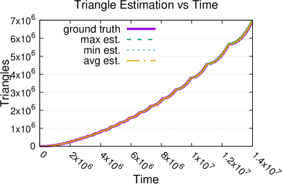
(a) Patent (Cit.)

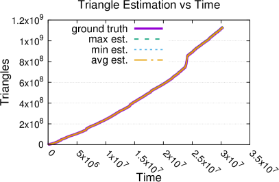
(b) LastFm

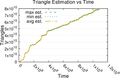
(c) Yahoo! Answers

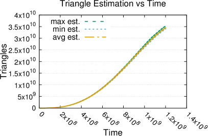
(d) Twitter

Figure 1: Estimation by trièst-impr of the global number of triangles over time (intended as number of elements seen on the stream). The max, min, and avg are taken over 10 runs. The curves are indistinguishable on purpose, to highlight the fact that trièst-impr estimations have very small error and variance. For example, the ground truth (for graphs for which it is available) is indistinguishable even from the max/min point-wise estimations over ten runs. For graphs for which the ground truth is not available, the small deviations from the avg suggest that the estimations are also close to the true value, given that our algorithms gives unbiased estimations.

Comparison with the state of the art

We compare quantitatively with three state-of-the-art methods: mascot [28], Jha et al. [20] and Pavan et al. [36]. mascot is a suite of local triangle counting methods (but provides also a global estimation). The other two are global triangle counting approaches. None of these can handle fully-dynamic streams, in contrast with trièst-fd. We first compare the three methods to trièst for the global triangle counting estimation. mascot comes in two memory efficient variants: the basic mascot-c variant and an improved mascot-i variant. Both variants sample edges with fixed probability $p$, so there is no guarantee on the amount of memory used during the execution. To ensure fairness of comparison, we devised the following experiment. First, we run both mascot-c and mascot-i for $\ell=10$ times with a fixed $p$ using the same random bits for the two algorithms run-by-run (i.e. the same coin tosses used to select the edges) measuring each time the number of edges $M^{\prime}_{i}$ stored in the sample at the end of the stream (by construction this the is same for the two variants run-by-run). Then, we run our algorithms using $M=M^{\prime}_{i}$ (for $i\in[\ell]$). We do the same to fix the size of the edge memory for Jha et al. [20] and Pavan et al. [36]. This way, all algorithms use the same amount of memory for storing edges (run-by-run).

We use the MAPE (Mean Average Percentage Error) to assess the accuracy of the global triangle estimators over time. The MAPE measures the average percentage of the prediction error with respect to the ground truth, and is widely used in the prediction literature [19]. For $t=1,\dotsc,T$, let $\overline{\Delta}^{(t)}$ be the estimator of the number of triangles at time $t$, the MAPE is defined as $\frac{1}{T}{\sum_{t=1}^{T}\left|\frac{|\Delta^{(t)}|-\overline{\Delta}^{(t)}}{|\Delta^{(t)}|}\right|}$.

In Fig. 2(a), we compare the average MAPE of trièst-base and trièst-impr as well as the two mascot variants and the other two streaming algorithms for the Patent (Co-Aut.) graph, fixing $p=0.01$. trièst-impr has the smallest error of all the algorithms compared.

We now turn our attention to the efficiency of the methods. Whenever we refer to one operation, we mean handling one element on the stream, either one edge addition or one edge deletion. The average update time per operation is obtained by dividing the total time required to process the entire stream by the number of operations (i.e., elements on the streams).

Figure 2(b) shows the average update time per operation in Patent (Co-Aut.) graph, fixing $p=0.01$. Both Jha et al. [20] and Pavan et al. [36] are up to $\approx 3$ orders of magnitude slower than the mascot variants and trièst. This is expected as both algorithms have an update complexity of $\Omega(M)$ (they have to go through the entire reservoir graph at each step), while both mascot algorithms and trièst need only to access the neighborhood of the nodes involved in the edge addition. This allows both algorithms to efficiently exploit larger memory sizes. We can use efficiently $M$ up to $1$ million edges in our experiments, which only requires few megabytes of RAM. mascot is one order of magnitude faster than trièst (which runs in $\approx 28$ micros/op), because it does not have to handle edge removal from the sample, as it offers no guarantees on the used memory. As we will show, trièst has much higher precision and scales well on billion-edges graphs.

Global triangle estimation MAPE for trièst and mascot. The rightmost column shows the reduction in terms of the avg. MAPE obtained by using trièst. Rows with $Y$ in column “Impr.” refer to improved algorithms (trièst-impr and mascot-i) while those with $N$ to basic algorithms (trièst-base and mascot-c). Max. MAPE Avg. MAPE Graph Impr. $p$ mascot trièst mascot trièst Change Patent (Cit.) N 0.01 0.9231 0.2583 0.6517 0.1811 -72.2% Y 0.01 0.1907 0.0363 0.1149 0.0213 -81.4% N 0.1 0.0839 0.0124 0.0605 0.0070 -88.5% Y 0.1 0.0317 0.0037 0.0245 0.0022 -91.1% Patent (Co-A.) N 0.01 2.3017 0.3029 0.8055 0.1820 -77.4% Y 0.01 0.1741 0.0261 0.1063 0.0177 -83.4% N 0.1 0.0648 0.0175 0.0390 0.0079 -79.8% Y 0.1 0.0225 0.0034 0.0174 0.0022 -87.2% LastFm N 0.01 0.1525 0.0185 0.0627 0.0118 -81.2% Y 0.01 0.0273 0.0046 0.0141 0.0034 -76.2% N 0.1 0.0075 0.0028 0.0047 0.0015 -68.1% Y 0.1 0.0048 0.0013 0.0031 0.0009 -72.1%

Given the slow execution of the other algorithms on the larger datasets we compare in details trièst only with mascot. Table 5.1 shows the average MAPE of the two approaches. The results confirm the pattern observed in Figure 2(a): trièst-base and trièst-impr both have an average error significantly smaller than that of the basic mascot-c and improved mascot variant respectively. We achieve up to a 91% (i.e., $9$-fold) reduction in the MAPE while using the same amount of memory. This experiment confirms the theory: reservoir sampling has overall lower or equal variance in all steps for the same expected total number of sampled edges.

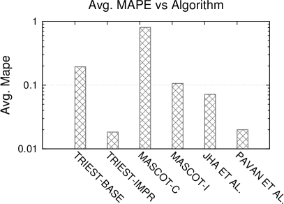
(a) MAPE

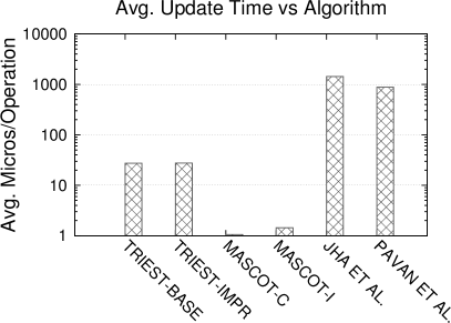
(b) Update Time

Figure 2: Average MAPE and average update time of the various methods on the Patent (Co-Aut.) graph with $p=0.01$ (for mascot, see the main text for how we computed the space used by the other algorithms) – insertion only. trièst-impr has the lowest error. Both Pavan et al. and Jha et al. have very high update times compared to our method and the two mascot variants.

To further validate this observation we run trièst-impr and the improved mascot-i variant using the same (expected memory) $M=10000$. Figure 3 shows the max-min estimation over $10$ runs and the standard deviation of the estimation over those runs. trièst-impr shows significantly lower standard deviation (hence variance) over the evolution of the stream, and the max and min lines are also closer to the ground truth. This confirms our theoretical observations in the previous sections. Even with very low $M$ (about $2/10000$ of the size of the graph) trièst gives high-quality estimations.

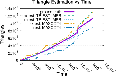
(a) Ground truth, max, and min

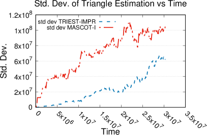
(b) Standard deviation

Figure 3: Accuracy and stability of the estimation of trièst-impr with $M=10000$ and of mascot-i with same expected memory, on LastFM, over 10 runs. trièst-impr has a smaller standard deviation and moreover the max/min estimation lines are closer to the ground truth. Average estimations not shown as they are qualitatively similar.

Local triangle counting

We compare the precision in local triangle count estimation of trièst with that of mascot [28] using the same approach of the previous experiment. We can not compare with Jha et al. and Pavan et al. algorithms as they provide only global estimation. As in [28], we measure the Pearson coefficient and the average $\varepsilon$ error (see [28] for definitions). In Table 5.1 we report the Pearson coefficient and average $\varepsilon$ error over all timestamps for the smaller graphs. trièst (significantly) improves (i.e., has higher correlation and lower error) over the state-of-the-art mascot, using the same amount of memory.

Comparison of the quality of the local triangle estimations between our algorithms and the state-of-the-art approach in [28]. Rows with $Y$ in column “Impr.” refer to improved algorithms (trièst-impr and mascot-i) while those with $N$ to basic algorithms (trièst-base and mascot-c). In virtually all cases we significantly outperform mascot using the same amount of memory. Avg. Pearson Avg. $\varepsilon$ Err. Graph Impr. $p$ mascot trièst Change mascot trièst Change LastFm Y 0.1 0.99 1.00 +1.18% 0.79 0.30 -62.02% 0.05 0.97 1.00 +2.48% 0.99 0.47 -52.79% 0.01 0.85 0.98 +14.28% 1.35 0.89 -34.24% N 0.1 0.97 0.99 +2.04% 1.08 0.70 -35.65% 0.05 0.92 0.98 +6.61% 1.32 0.97 -26.53% 0.01 0.32 0.70 +117.74% 1.48 1.34 -9.16% Patent (Cit.) Y 0.1 0.41 0.82 +99.09% 0.62 0.37 -39.15% 0.05 0.24 0.61 +156.30% 0.65 0.51 -20.78% 0.01 0.05 0.18 +233.05% 0.65 0.64 -1.68% N 0.1 0.16 0.48 +191.85% 0.66 0.60 -8.22% 0.05 0.06 0.24 +300.46% 0.67 0.65 -3.21% 0.01 0.00 0.003 +922.02% 0.86 0.68 -21.02% Patent (Co-aut.) Y 0.1 0.55 0.87 +58.40% 0.86 0.45 -47.91% 0.05 0.34 0.71 +108.80% 0.91 0.63 -31.12% 0.01 0.08 0.26 +222.84% 0.96 0.88 -8.31% N 0.1 0.25 0.52 +112.40% 0.92 0.83 -10.18% 0.05 0.09 0.28 +204.98% 0.92 0.92 0.10% 0.01 0.01 0.03 +191.46% 0.70 0.84 20.06%

Memory vs accuracy trade-offs

We study the trade-off between the sample size $M$ vs the running time and accuracy of the estimators. Figure 4(a) shows the tradeoffs between the accuracy of the estimation (as MAPE) and the size $M$ for the smaller graphs for which the ground truth number of triangles can be computed exactly using the naïve algorithm. Even with small $M$, trièst-impr achieves very low MAPE value. As expected, larger $M$ corresponds to higher accuracy and for the same $M$ trièst-impr outperforms trièst-base.

Figure 4(b) shows the average time per update in microseconds ($\mu$s) for trièst-impr as function of $M$. Some considerations on the running time are in order. First, a larger edge sample (larger $M$) generally requires longer average update times per operation. This is expected as a larger sample corresponds to a larger sample graph on which to count triangles. Second, on average a few hundreds microseconds are sufficient for handling any update even in very large graphs with billions of edges. Our algorithms can handle hundreds of thousands of edge updates (stream elements) per second, with very small error (Fig. 4(a)), and therefore trièst can be used efficiently and effectively in high-velocity contexts. The larger average time per update for Patent (Co-Auth.) can be explained by the fact that the graph is relatively dense and has a small size (compared to the larger Yahoo! and Twitter graphs). More precisely, the average time per update (for a fixed $M$) depends on two main factors: the average degree and the length of the stream. The denser the graph is, the higher the update time as more operations are needed to update the triangle count every time the sample is modified. On the other hand, the longer the stream, for a fixed $M$, the lower is the frequency of updates to the reservoir (it can be show that the expected number of updates to the reservoir is $O(M(1+\log(\frac{t}{M})))$ which grows sub-linearly in the size of the stream $t$). This explains why the average update time for the large and dense Yahoo! and Twitter graphs is so small, allowing the algorithm to scale to billions of updates.

(a) $M$ vs MAPE

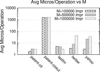
(b) $M$ vs Update Time (trièst-impr)

Figure 4: Trade-offs between $M$ and MAPE and avg. update time ($\mu$s) – edge insertion only. Larger $M$ implies lower errors but generally higher update times.

Alternative edge orders

In all previous experiments the edges are added in their natural order (i.e., in order of their appearance). While the natural order is the most important use case, we have assessed the impact of other ordering on the accuracy of the algorithms. We experiment with both the uniform-at-random (u.a.r.) order of the edges and the random BFS order: until all the graph is explored a BFS is started from a u.a.r. unvisited node and edges are added in order of their visit (neighbors are explored in u.a.r. order). The results for the random BFS order and u.a.r. order (Fig. 5) confirm that trièst has the lowest error and is very scalable in every tested ordering.

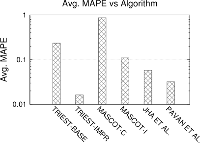
(a) BFS order

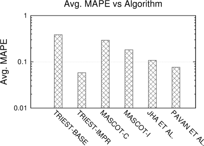
(b) U.a.r. order

Figure 5: Average MAPE on Patent (Co-Aut.), with $p=0.01$ (for mascot, see the main text for how we computed the space used by the other algorithms) – insertion only in Random BFS order and in u.a.r. order. trièst-impr has the lowest error.

5.2 Fully-dynamic case

We evaluate trièst-fd on fully-dynamic streams. We cannot compare trièst-fd with the algorithms previously used [20, 36, 28] as they only handle insertion-only streams.

In the first set of experiments we model deletions using the widely used sliding window model, where a sliding window of the most recent edges defines the current graph. The sliding window model is of practical interest as it allows to observe recent trends in the stream. For Patent (Co-Aut.) & (Cit.) we keep in the sliding window the edges generated in the last $5$ years, while for LastFm we keep the edges generated in the last $30$ days. For Yahoo! Answers we keep the last $100$ millions edges in the window.

Figure 6 shows the evolution of the global number of triangles in the sliding window model using trièst-fd using $M=200{,}000$ ($M=1{,}000{,}000$ for Yahoo! Answers). The sliding window scenario is significantly more challenging than the addition-only case (very often the entire sample of edges is flushed away) but trièst-fd maintains good variance and scalability even when, as for LastFm and Yahoo! Answers, the global number of triangles varies quickly.

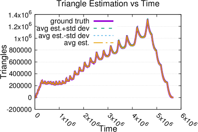
(a) Patent (Co-Aut.)

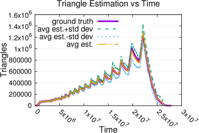
(b) Patent (Cit.)

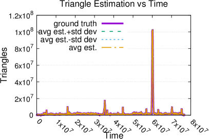
(c) LastFm

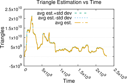
(d) Yahoo! Answers

Figure 6: Evolution of the global number of triangles in the fully-dynamic case (sliding window model for edge deletion). The curves are indistinguishable on purpose, to remark the fact that trièst-fd estimations are extremely accurate and consistent. We comment on the observed patterns in the text.

Continuous monitoring of triangle counts with trièst-fd allows to detect patterns that would otherwise be difficult to notice. For LastFm (Fig. 6(c)) we observe a sudden spike of several order of magnitudes. The dataset is anonymized so we cannot establish which songs are responsible for this spike. In Yahoo! Answers (Fig. 6(d)) a popular topic can create a sudden (and shortly lived) increase in the number of triangles, while the evolution of the Patent co-authorship and co-citation networks is slower, as the creation of an edge requires filing a patent (Fig. 6(a) and (b)). The almost constant increase over time of the number of triangles in Patent graphs is consistent with previous observations of densification in collaboration networks as in the case of nodes’ degrees [27] and the observations on the density of the densest subgraph [15].

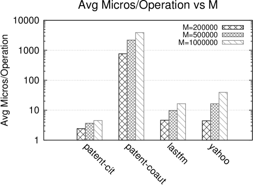
Figure 7: Trade-offs between the avg. update time ($\mu$s) and $M$ for trièst-fd.

Table 5.2 shows the results for both the local and global triangle counting estimation provided by trièst-fd. In this case we can not compare with previous works, as they only handle insertions. It is evident that precision improves with $M$ values, and even relatively small $M$ values result in a low MAPE (global estimation), high Pearson correlation and low $\varepsilon$ error (local estimation). Figure 7 shows the tradeoffs between memory (i.e., accuracy) and time. In all cases our algorithm is very fast and it presents update times in the order of hundreds of microseconds for datasets with billions of updates (Yahoo! Answers).

Estimation errors for trièst-fd. Avg. Global Avg. Local Graph $M$ MAPE Pearson $\varepsilon$ Err. LastFM 200000 0.005 0.980 0.020 1000000 0.002 0.999 0.001 Pat. (Co-Aut.) 200000 0.010 0.660 0.300 1000000 0.001 0.990 0.006 Pat. (Cit.) 200000 0.170 0.090 0.160 1000000 0.040 0.600 0.130

Alternative models for deletion

We evaluate trièst-fd using other models for deletions than the sliding window model. To assess the resilience of the algorithm to massive deletions we run the following experiments. We added edges in their natural order but each edge addition is followed with probability $q$ by a mass deletion event where each edge currently in the the graph is deleted with probability $d$ independently. We run experiments with $q=3{,}000{,}000^{-1}$ (i.e., a mass deletion expected every $3$ millions edges) and $d=0.80$ (in expectation $80\%$ of edges are deleted). The results are shown in Table 5.2.

Estimation errors for trièst-fd– mass deletion experiment, $q=3{,}000{,}000^{-1}$ and $d=0.80$. Avg. Global Avg. Local Graph $M$ MAPE Pearson $\varepsilon$ Err. LastFM 200000 0.040 0.620 0.53 1000000 0.006 0.950 0.33 Pat. (Co-Aut.) 200000 0.060 0.278 0.50 1000000 0.006 0.790 0.21 Pat. (Cit.) 200000 0.280 0.068 0.06 1000000 0.026 0.510 0.04

We observe that trièst-fd maintains a good accuracy and scalability even in face of a massive (and unlikely) deletions of the vast majority of the edges: e.g., for LastFM with $M=200000$ (resp. $M=1{,}000{,}000$) we observe $0.04$ (resp. $0.006$) Avg. MAPE.

6 Conclusions

We presented trièst, the first suite of algorithms that use reservoir sampling and its variants to continuously maintain unbiased, low-variance estimates of the local and global number of triangles in fully-dynamic graphs streams of arbitrary edge/vertex insertions and deletions using a fixed, user-specified amount of space. Our experimental evaluation shows that trièst outperforms state-of-the-art approaches and achieves high accuracy on real-world datasets with more than one billion of edges, with update times of hundreds of microseconds.

APPENDIX

Appendix A Additional theoretical results

In this section we present the theoretical results (statements and proofs) not included in the main body.

A.1 Theoretical results for trièst-base

Before proving Lemma 4.1, we need to introduce the following lemma, which states a well known property of the reservoir sampling scheme.

Lemma A.1 ([42, Sect. 2]).

For any $t>M$, let $A$ be any subset of $E^{(t)}$ of size $|A|=M$. Then, at the end of time step $t$,

$$\Pr(\mathcal{S}=A)=\frac{1}{\binom{|E^{(t)}|}{M}}=\frac{1}{\binom{t}{M}},$$

i.e., the set of edges in $\mathcal{S}$ at the end of time $t$ is a subset of $E^{(t)}$ of size $M$ chosen uniformly at random from all subsets of $E^{(t)}$ of the same size.

Proof A.2 (of Lemma 4.1).

If $k>\min\{M,t\}$, we have $\Pr(B\subseteq\mathcal{S})=0$ because it is impossible for $B$ to be equal to $\mathcal{S}$ in these cases. From now on we then assume $k\leq\min\{M,t\}$.

If $t\leq M$, then $E^{(t)}\subseteq\mathcal{S}$ and $\Pr(B\subseteq\mathcal{S})=1=\xi_{k,t}^{-1}$.

Assume instead that $t>M$, and let $\mathcal{B}$ be the family of subsets of $E^{(t)}$ that 1. have size $M$, and 2. contain $B$:

$$\mathcal{B}=\{C\subset E^{(t)}~{}:~{}|C|=M,B\subseteq C\}\enspace.$$

We have

$$|\mathcal{B}|=\binom{|E^{(t)}|-k}{M-k}=\binom{t-k}{M-k}\enspace.$$ (15)

From this and and Lemma A.1 we then have

$$\Pr(B\subseteq\mathcal{S}) =\Pr(\mathcal{S}\in\mathcal{B})=\sum_{C\in\mathcal{B}}\Pr(\mathcal{S}=C)$$

$$=\frac{\binom{t-k}{M-k}}{\binom{t}{M}}=\frac{\binom{t-k}{M-k}}{\binom{t-k}{M-k}\prod_{i=0}^{k-1}\frac{t-i}{M-i}}=\prod_{i=0}^{k-1}\frac{M-i}{t-i}=\xi_{k,t}^{-1}\enspace.$$

A.1.1 Expectation

Proof A.3 (of Lemma 4.3).

We only show the proof for $\tau$, as the proof for the local counters follows the same steps.

The proof proceeds by induction. The thesis is true after the first call to UpdateCounters at time $t=1$. Since only one edge is in $\mathcal{S}$ at this point, we have $\Delta^{\mathcal{S}}=0$, and $\mathcal{N}^{\mathcal{S}}_{u,v}=\emptyset$, so UpdateCounters does not modify $\tau$, which was initialized to $0$. Hence $\tau=0=\Delta^{\mathcal{S}}$.

Assume now that the thesis is true for any subsequent call to UpdateCounters up to some point in the execution of the algorithm where an edge $(u,v)$ is inserted or removed from $\mathcal{S}$. We now show that the thesis is still true after the call to UpdateCounters that follows this change in $\mathcal{S}$. Assume that $(u,v)$ was inserted in $\mathcal{S}$ (the proof for the case of an edge being removed from $\mathcal{S}$ follows the same steps). Let $\mathcal{S}^{\mathrm{b}}=\mathcal{S}\setminus\{(u,v)\}$ and $\tau^{\mathrm{b}}$ be the value of $\tau$ before the call to UpdateCounters and, for any $w\in V_{\mathcal{S}^{\mathrm{b}}}$, let $\tau_{w}^{\mathrm{b}}$ be the value of $\tau_{w}$ before the call to UpdateCounters. Let $\Delta^{\mathcal{S}}_{u,v}$ be the set of triangles in $G_{\mathcal{S}}$ that have $u$ and $v$ as corners. We need to show that, after the call, $\tau=|\Delta^{\mathcal{S}}|$. Clearly we have $\Delta^{\mathcal{S}}=\Delta^{\mathcal{S}^{\mathrm{b}}}\cup\Delta^{\mathcal{S}}_{u,v}$ and $\Delta^{\mathcal{S}^{\mathrm{b}}}\cap\Delta^{\mathcal{S}}_{u,v}=\emptyset$, so

$$|\Delta^{\mathcal{S}}|=|\Delta^{\mathcal{S}^{\mathrm{b}}}|+|\Delta^{\mathcal{S}}_{u,v}|$$

We have $|\Delta^{\mathcal{S}}_{u,v}|=|\mathcal{N}^{\mathcal{S}}_{u,v,}|$ and, by the inductive hypothesis, we have that $\tau^{\mathrm{b}}=|\Delta^{\mathcal{S}^{\mathrm{b}}}|$. Since UpdateCounters increments $\tau$ by $|\mathcal{N}^{\mathcal{S}}_{u,v,}|$, the value of $\tau$ after UpdateCounters has completed is exactly $|\Delta^{\mathcal{S}}|$.

We can now prove Thm. 4.2 on the unbiasedness of the estimation computed by trièst-base (and on their exactness for $t\leq M$).

Proof A.4 (of Thm. 4.2).

We prove the statement for the estimation of global triangle count. The proof for the local triangle counts follows the same steps.

If $t\leq M$, we have $G_{\mathcal{S}}=G^{(t)}$ and from Lemma 4.3 we have $\tau^{(t)}=|\Delta^{\mathcal{S}}|=|\Delta^{(t)}|$, hence the thesis holds.

Assume now that $t>M$, and assume that $|\Delta^{(t)}|>0$, otherwise, from Lemma 4.3, we have $\tau^{(t)}=|\Delta^{\mathcal{S}}|=0$ and trièst-base estimation is deterministically correct. Let $\lambda=(a,b,c)\in\Delta^{(t)}$, (where $a,b,c$ are edges in $E^{(t)}$) and let $\delta_{\lambda}^{(t)}$ be a random variable that takes value $\xi^{(t)}$ if $\lambda\in\Delta_{\mathcal{S}}$ (i.e., $\{a,b,c\}\subseteq\mathcal{S}$) at the end of the step instant $t$, and $0$ otherwise. From Lemma 4.1, we have that

$$\mathbb{E}\left[\delta_{\lambda}^{(t)}\right]=\xi^{(t)}\Pr(\{a,b,c\}\subseteq\mathcal{S})=\xi^{(t)}\frac{1}{\xi_{3,t}}=\xi^{(t)}\frac{1}{\xi^{(t)}}=1\enspace.$$ (16)

We can write

$$\xi^{(t)}\tau^{(t)}=\sum_{\lambda\in\Delta^{(t)}}\delta_{\lambda}^{(t)}$$

and from this, (16), and linearity of expectation, we have

$$\mathbb{E}\left[\xi^{(t)}\tau^{(t)}\right]=\sum_{\lambda\in\Delta^{(t)}}\mathbb{E}\left[\delta_{\lambda}^{(t)}\right]=|\Delta^{(t)}|\enspace.$$

A.1.2 Concentration

Proof A.5 (of Lemma 4.9).

Using the law of total probability, we have

$$\Pr\left(f(\mathcal{S}_{\textsc{in}})=1\right) =\sum_{k=0}^{t}\Pr\left(f(\mathcal{S}_{\textsc{in}})=1~{}\left|~{}|\mathcal{S}_{\textsc{in}}|=k\right.\right)\Pr(|\mathcal{S}_{\textsc{in}}|=k)$$

$$\geq\Pr\left(f(\mathcal{S}_{\textsc{in}})=1~{}\left|~{}|\mathcal{S}_{\textsc{in}}|=M\right.\right)\Pr(|\mathcal{S}_{\textsc{in}}|=M)$$

$$\geq\Pr\left(f(\mathcal{S}_{\textsc{mix}})=1\right)\Pr\left(|\mathcal{S}_{\textsc{in}}|=M\right),$$ (17)

where the last inequality comes from Lemma A.1: the set of edges included in $\mathcal{S}_{\textsc{mix}}$ is a uniformly-at-random subset of $M$ edges from $E^{(t)}$, and the same holds for $\mathcal{S}_{\textsc{in}}$ when conditioning its size being $M$.

Using the Stirling approximation $\sqrt{2\pi n}(\frac{n}{e})^{n}\leq n!\leq e\sqrt{n}(\frac{n}{e})^{n}$ for any positive integer $n$, we have

$$\Pr\left(|\mathcal{S}_{\textsc{in}}|=M\right) =\binom{t}{M}\left(\frac{M}{t}\right)^{M}\left(\frac{t-M}{t}\right)^{t-M}$$

$$\geq\frac{t^{t}\sqrt{t}\sqrt{2\pi}e^{-t}}{e^{2}\sqrt{M}\sqrt{t-M}e^{-t}M^{M}(t-M)^{t-M}}\frac{M^{M}(t-M)^{t-M}}{t^{t}}$$

$$\geq\frac{1}{e\sqrt{M}}\enspace.$$

Plugging this into (17) concludes the proof.

Fact 2.

For any $x>2$, we have

$$\frac{x^{2}}{(x-1)(x-2)}\leq 1+\frac{4}{x-2}\enspace.$$

Proof A.6 (of Lemma 4.12).

We start by looking at the ratio between $\frac{t(t-1)(t-2)}{M(M-1)(M-2)}$ and $(t/M)^{3}$. We have:

$$1\leq\frac{t(t-1)(t-2)}{M(M-1)(M-2)}\left(\frac{M}{t}\right)^{3} =\frac{M^{2}}{(M-1)(M-2)}\frac{(t-1)(t-2)}{t^{2}}$$

$$\leq\frac{M^{2}}{(M-1)(M-2)}$$

$$\leq 1+\frac{4}{M-2}$$

where the last step follows from Fact 2. Using this, we obtain

$$\left|\phi^{(t)}-\phi_{\textsc{mix}}^{(t)}\right| =\left|\tau^{(t)}\frac{t(t-1)(t-2)}{M(M-1)(M-2)}-\tau^{(t)}\left(\frac{t}{M}\right)^{3}\right|$$

$$=\left|\tau^{(t)}\left(\frac{t}{M}\right)^{3}\left(\frac{t(t-1)(t-2)}{M(M-1)(M-2)}\left(\frac{M}{t}\right)^{3}-1\right)\right|$$

$$\leq\tau^{(t)}\left(\frac{t}{M}\right)^{3}\frac{4}{M-2}$$

$$=\phi_{\textsc{mix}}^{(t)}\frac{4}{M-2}\enspace.$$

A.1.3 Variance comparison

We now prove Lemma 4.14, about the fact that the variance of the estimations computed by trièst-base is smaller, for most of the stream, than the variance of the estimations computed by mascot-c [28]. We first need the following technical fact.

Fact 3.

For any $x>42$, we have

$$\frac{x^{2}}{(x-3)(x-4)}\leq 1+\frac{8}{x}\enspace.$$

Proof A.7 (of Lemma 4.14).

We focus on $t>M>42$ otherwise the theorem is immediate. We show that for such conditions $f(M,t)<\bar{f}(M/T)$ and $g(M,t)<\bar{g}(M/T)$. Using the fact that $t\leq\alpha T$ and Fact 2, we have

$$f(M,t)-\bar{f}(M/T) =\frac{t(t-1)(t-2)}{M(M-1)(M-2)}-\frac{T^{3}}{M^{3}}$$

$$<\frac{\alpha^{3}T^{3}}{M^{3}}\frac{M^{2}}{(M-1)(M-2)}-\frac{T^{3}}{M^{3}}$$

$$\leq\frac{\alpha^{3}T^{3}}{M^{3}}\left(1+\frac{4}{M-2}\right)-\frac{T^{3}}{M^{3}}$$

$$\leq\frac{T^{3}}{M^{3}}\left(\alpha^{3}+\frac{4\alpha^{3}}{M-2}-1\right)\enspace.$$ (18)

Given that $T$ and $M$ are $\geq 42$, the r.h.s. of (18) is non-positive iff

$$\alpha^{3}+\frac{4\alpha^{3}}{M-2}-1\leq 0\enspace.$$

Solving for $M$ we have that the above is verified when $M\geq\frac{4\alpha^{3}}{1-\alpha^{3}}+2$. This is always true given our assumption that $M>\max(\frac{8\alpha}{1-\alpha},42)$: for any $0<\alpha<0.6$, we have $\frac{4\alpha^{3}}{1-\alpha^{3}}+2<42\leq M$ and for any $0.6\leq\alpha<1$ we have $\frac{4\alpha^{3}}{1-\alpha^{3}}+2<\frac{8\alpha}{1-\alpha}\leq M$. Hence the r.h.s. of (18) is $\leq 0$ and $f(M,t)<\bar{f}(M/T)$.

We also have:

$$g(M,t)-\bar{g}(M/T) =\frac{t(t-1)(t-2)(M-3)(M-4)}{(t-3)(t-4)M(M-1)(M-2)}-\frac{T}{M}$$

$$<\frac{t}{M}\frac{t^{2}}{(t-3)(t-4)}-\frac{T}{M}$$

$$\leq\frac{t}{M}\left(1+\frac{8}{t}\right)-\frac{T}{M},$$ (19)

where the last inequality follow from Fact 3, since $t>M>42$. Now, from (19) since $t\leq\alpha T$ and $t>M$, we can write:

$$g(M,t)-\bar{g}(M/T)<\frac{T}{M}\left(\alpha+\frac{8\alpha}{M}-1\right)\enspace.$$

The r.h.s. of this equation is non-positive given the assumption $M>\frac{8\alpha}{1-\alpha}$, hence $g(M,t)<\bar{g}(M/T)$.

A.2 Theoretical results for trièst-impr

A.2.1 Expectation

Proof A.8 (of Thm. 4.15).

If $t\leq M$ trièst-impr behaves exactly like trièst-base, and the statement follows from Lemma 4.2.

Assume now $t>M$ and assume that $|\Delta^{(t)}|>0$, otherwise, the algorithm deterministically returns $0$ as an estimation and the thesis follows. Let $\lambda\in\Delta^{(t)}$ and denote with $a$, $b$, and $c$ the edges of $\lambda$ and assume, w.l.o.g., that they appear in this order (not necessarily consecutively) on the stream. Let $t_{\lambda}$ be the time step at which $c$ is on the stream. Let $\delta_{\lambda}$ be a random variable that takes value $\xi_{2,t_{\lambda}-1}$ if $a$ and $b$ are in $\mathcal{S}$ at the end of time step $t_{\lambda}-1$, and $0$ otherwise. Since it must be $t_{\lambda}-1\geq 2$, from Lemma 4.1 we have that

$$\Pr\left(\delta_{\lambda}=\xi_{2,t_{\lambda}-1}\right)=\frac{1}{\xi_{2,t_{\lambda}-1}}\enspace.$$ (20)

When $c=(u,v)$ is on the stream, i.e., at time $t_{\lambda}$, trièst-impr calls UpdateCounters and increments the counter $\tau$ by $|\mathcal{N}^{\mathcal{S}}_{u,v}|\xi_{2,t_{\lambda}-1}$, where $|\mathcal{N}^{\mathcal{S}}_{u,v}|$ is the number of triangles with $(u,v)$ as an edge in $\Delta^{\mathcal{S}\cup\{c\}}$. All these triangles have the corresponding random variables taking the same value $\xi_{2,t_{\lambda}-1}$. This means that the random variable $\tau^{(t)}$ can be expressed as

$$\tau^{(t)}=\sum_{\lambda\in\Delta^{(t)}}\delta_{\lambda}\enspace.$$

From this, linearity of expectation, and (20), we get

$$\mathbb{E}\left[\tau^{(t)}\right]=\sum_{\lambda\in\Delta^{(t)}}\mathbb{E}[\delta_{\lambda}]=\sum_{\lambda\in\Delta^{(t)}}\xi_{2,t_{\lambda}-1}\Pr\left(\delta_{\lambda}=\xi_{2,t_{\lambda}-1}\right)=\sum_{\lambda\in\Delta^{(t)}}\xi_{2,t_{\lambda}-1}\frac{1}{\xi_{2,t_{\lambda}-1}}=|\Delta^{(t)}|\enspace.$$

A.2.2 Variance

Proof A.9 (of Lemma 4.17).

Consider first the case where all edges of $\lambda$ appear on the stream before any edge of $\gamma$, i.e.,

$$t_{\ell_{1}}<t_{\ell_{2}}<t_{\ell_{3}}<t_{g_{1}}<t_{g_{2}}<t_{g_{3}}\enspace.$$

The presence or absence of either or both $\ell_{1}$ and $\ell_{2}$ in $\mathcal{S}$ at the beginning of time step $t_{\ell_{3}}$ (i.e., whether $D_{\lambda}$ happens or not) has no effect whatsoever on the probability that $g_{1}$ and $g_{2}$ are in the sample $\mathcal{S}$ at the beginning of time step $t_{g_{3}}$. Hence in this case,

$$\Pr(D_{\gamma}~{}|~{}D_{\lambda})=\Pr(D_{\gamma})\enspace.$$

Consider now the case where, for any $i\in\{1,2\}$, the edges $g_{1},\dotsc,g_{i}$ appear on the stream before $\ell_{3}$ does. Define now the events

• $A_{i}$: “the edges $g_{1},\dotsc,g_{i}$ are in the sample $\mathcal{S}$ at the beginning of time step $t_{\ell_{3}}$.”

• $B_{i}$: if $i=1$, this is the event “the edge $g_{2}$ is inserted in the sample $\mathcal{S}$ during time step $t_{g_{2}}$.” If $i=2$, this event is the whole event space, i.e., the event that happens with probability $1$.

• $C$: “neither $g_{1}$ nor $g_{2}$ were among the edges removed from $\mathcal{S}$ between the beginning of time step $t_{\ell_{3}}$ and the beginning of time step $t_{g_{3}}$.”

We can rewrite $D_{\gamma}$ as

$$D_{\gamma}=A_{i}\cap B_{i}\cap C\enspace.$$

Hence

$$\Pr(D_{\gamma}~{}|~{}D_{\lambda}) =\Pr\left(A_{i}\cap B_{i}\cap C~{}|~{}D_{\lambda}\right)$$

$$=\Pr\left(A_{i}~{}|~{}D_{\lambda}\right)\Pr\left(B_{i}\cap C~{}|~{}A_{i}\cap D_{\lambda}\right)\enspace.$$ (21)

We now show that

$$\Pr\left(A_{i}~{}|~{}D_{\lambda}\right)\leq\Pr\left(A_{i}\right)\enspace.$$

If we assume that $t_{\ell_{3}}\leq M+1$, then all the edges that appeared on the stream up until the beginning of $t_{\ell_{3}}$ are in $\mathcal{S}$. Therefore,

$$\Pr\left(A_{i}~{}|~{}D_{\lambda}\right)=\Pr(A_{i})=1\enspace.$$

Assume instead that $t_{\ell_{3}}>M+1$. Among the $\binom{t_{\ell_{3}}-1}{M}$ subsets of $E^{(t_{\ell_{3}}-1)}$ of size $M$, there are $\binom{t_{\ell_{3}}-3}{M-2}$ that contain $\ell_{1}$ and $\ell_{2}$. From Lemma A.1, we have that at the beginning of time $t_{\ell_{3}}$, $\mathcal{S}$ is a subset of size $M$ of $E^{(t_{\ell_{3}}-1)}$ chosen uniformly at random. Hence, if we condition on the fact that $\{\ell_{1},\ell_{2}\}\subset\mathcal{S}$, we have that $\mathcal{S}$ is chosen uniformly at random from the $\binom{t_{\ell_{3}}-3}{M-2}$ subsets of $E^{(t_{\ell_{3}}-1)}$ of size $M$ that contain $\ell_{1}$ and $\ell_{2}$. Among these, there are $\binom{t_{\ell_{3}}-3-i}{M-2-i}$ that also contain $g_{1},\dotsc,g_{i}$. Therefore,

$$\Pr(A_{i}~{}|~{}D_{\lambda})=\frac{\binom{t_{\ell_{3}}-3-i}{M-2-i}}{\binom{t_{\ell_{3}}-3}{M-2}}=\prod_{j=0}^{i-1}\frac{M-2-j}{t_{\ell_{3}}-3-j}\enspace.$$

From Lemma 4.1 we have

$$\Pr(A_{i})=\frac{1}{\xi_{i,t_{\ell_{3}}-1}}=\prod_{j=0}^{i-1}\frac{M-j}{t_{\ell_{3}}-1-j},$$

where the last equality comes from the assumption $t_{\ell_{3}}>M+1$. From the same assumption and from the fact that for any $j\geq 0$ and any $y\geq x>j$ it holds $\frac{x-j}{y-j}\leq\frac{x}{y}$, then we have

$$\Pr(A_{i}~{}|~{}D_{\lambda})\leq\Pr(A_{i})\enspace.$$

This implies, from (A.9), that

$$\Pr(D_{\gamma}~{}|~{}D_{\lambda})\leq\Pr(A_{i})\Pr(B_{i}\cap C~{}|~{}A_{i}\cap D_{\lambda})\enspace.$$ (22)

Consider now the events $B_{i}$ and $C$. When conditioned on $A_{i}$, these event are both independent from $D_{\lambda}$: if the edges $g_{1},\dotsc,g_{i}$ are in $\mathcal{S}$ at the beginning of time $t_{\ell_{3}}$, the fact that the edges $\ell_{1}$ and $\ell_{2}$ were also in $\mathcal{S}$ at the beginning of time $t_{\ell_{3}}$ has no influence whatsoever on the actions of the algorithm (i.e., whether an edge is inserted in or removed from $\mathcal{S}$). Thus,

$$\Pr(A_{i})\Pr(B_{i}\cap C~{}|~{}A_{i}\cap D_{\lambda})=\Pr(A_{i})\Pr(B_{i}\cap C~{}|~{}A_{i})\enspace.$$

Putting this together with (22), we obtain

$$\Pr(D_{\gamma}~{}|~{}D_{\lambda})\leq\Pr(A_{i})\Pr(B_{i}\cap C~{}|~{}A_{i})\leq\Pr(A_{i}\cap B_{i}\cap C)\leq\Pr(D_{\gamma})\enspace,$$

where the last inequality follows from the fact that $D_{\gamma}=A_{i}\cap B_{i}\cap C$ by definition.

A.3 Theoretical results for trièst-fd

A.3.1 Expectation

Before proving Thm. 4.21 we need the following technical lemmas.

The following is a corollary of [16, Thm. 1].

Lemma A.10.

For any $t>0$, and any $j$, $0\leq j\leq s^{(t)}$, let $\mathcal{B}^{(t)}$ be the collection of subsets of $E^{(t)}$ of size $j$. For any $B\in\mathcal{B}^{(t)}$ it holds

$$\Pr\left(\mathcal{S}=B~{}|~{}M^{(t)}=j\right)=\frac{1}{\binom{|E^{(t)}|}{j}}\enspace.$$

That is, conditioned on its size at the end of time step $t$, $\mathcal{S}$ is equally likely to be, at the end of time step $t$, any of the subsets of $E^{(t)}$ of that size.

The next lemma is an immediate corollary of [16, Thm. 2]

Lemma A.11.

Recall the definition of $\kappa^{(t)}$ from (14). We have

$$\kappa^{(t)}=\Pr(M^{(t)}\geq 3)\enspace.$$

The next lemma follows from Lemma A.10 in the same way as Lemma 4.1 follows from Lemma A.1.

Lemma A.12.

For any time step $t$ and any $j$, $0\leq j\leq s^{(t)}$, let $B$ be any subset of $E^{(t)}$ of size $|B|=k\leq s^{(t)}$. Then, at the end of time step $t$,

$$\Pr\left(B\subseteq\mathcal{S}~{}|~{}M^{(t)}=j\right)=\left\{\begin{array}[]{cl}0&\text{if }k>j\\ \displaystyle\frac{1}{\psi_{k,j,s^{(t)}}}&\text{otherwise}\end{array}\right.\enspace.$$

The next two lemmas discuss properties of trièst-fd for $t<t^{*}$, where $t^{*}$ is the first time that $|E^{(t)}|$ had size $M+1$ ($t^{*}\geq M+1$).

Lemma A.13.

For all $t<t^{*}$, we have:

1. $d_{\mathrm{o}}^{(t)}=0$; and

2. $\mathcal{S}=E^{(t)}$; and

3. $M^{(t)}=s^{(t)}$.

Proof A.14.

Since the third point in the thesis follows immediately from the second, we focus on the first two points.

The proof is by induction on $t$. In the base base for $t=1$: the element on the stream must be an insertion, and the algorithm deterministically inserts the edge in $\mathcal{S}$. Assume now that it is true for all time steps up to (but excluding) some $t\leq t^{*}-1$. We now show that it is also true for $t$.

Assume the element on the stream at time $t$ is a deletion. The corresponding edge must be in $\mathcal{S}$, from the inductive hypothesis. Hence trièst-fd removes it from $\mathcal{S}$ and increments the counter $d_{\mathrm{i}}$ by 1. Thus it is still true that $\mathcal{S}=E^{(t)}$ and $d_{\mathrm{o}}^{(t)}=0$, and the thesis holds.

Assume now that the element on the stream at time $t$ is an insertion. From the inductive hypothesis we have that the current value of the counter $d_{\mathrm{o}}$ is 0.

If the counter $d_{\mathrm{i}}$ has currently value 0 as well, then, because of the hypothesis that $t<t^{*}$, it must be that $|\mathcal{S}|=M^{(t-1)}=s^{(t-1)}<M$. Therefore trièst-fd always inserts the edge in $\mathcal{S}$. Thus it is still true that $\mathcal{S}=E^{(t)}$ and $d_{\mathrm{o}}^{(t)}=0$, and the thesis holds.

If otherwise $d_{\mathrm{i}}>0$, then trièst-fd flips a biased coin with probability of heads equal to

$$\frac{d_{\mathrm{i}}}{d_{\mathrm{i}}+d_{\mathrm{o}}}=\frac{d_{\mathrm{i}}}{d_{\mathrm{i}}}=1,$$

therefore trièst-fd always inserts the edge in $\mathcal{S}$ and decrements $d_{\mathrm{i}}$ by one. Thus it is still true that $\mathcal{S}=E^{(t)}$ and $d_{\mathrm{o}}^{(t)}=0$, and the thesis holds.

The following result is an immediate consequence of Lemma A.11 and Lemma A.13.

Lemma A.15.

For all $t<t^{*}$ such that $s^{(t)}\geq 3$, we have $\kappa^{(t)}=1$.

We can now prove Thm. 4.21.

Proof A.16 (of Thm. 4.21).

Assume for now that $t<t^{*}$. From Lemma A.13, we have that $s^{(t)}=M^{(t)}$. If $M^{(t)}<3$, then it must be $s^{(t)}<3$, hence $|\Delta^{(t)}|=0$ and indeed the algorithm returns $\rho^{(t)}=0$ in this case. If instead $M^{(t)}=s^{(t)}\geq 3$, then we have

$$\rho^{(t)}=\frac{\tau^{(t)}}{\kappa^{(t)}}\enspace.$$

From Lemma A.15 we have that $\kappa^{(t)}=1$ for all $t<t^{*}$, hence $\rho^{(t)}=\tau^{(t)}$ in these cases. Since (an identical version of) Lemma 4.3 also holds for trièst-fd, we have $\tau^{(t)}=|\Delta^{\mathcal{S}}|=|\Delta^{(t)}|$, where the last equality comes from the fact that $\mathcal{S}=E^{(t)}$ (Lemma A.13). Hence $\rho^{(t)}=|\Delta^{(t)}|$ for any $t\leq t^{*}$, as in the thesis.

Assume now that $t\geq t^{*}$. Using the law of total expectation, we can write

$$\mathbb{E}\left[\rho^{(t)}\right]=\sum_{j=0}^{\min\{s^{(t)},M\}}\mathbb{E}\left[\rho^{(t)}~{}|~{}M^{(t)}=j\right]\Pr\left(M^{(t)}=j\right)\enspace.$$ (23)

Assume that $|\Delta^{(t)}|>0$, otherwise, the algorithm deterministically returns $0$ as an estimation and the thesis follows. Let $\lambda$ be a triangle in $\Delta^{(t)}$, and let $\delta_{\lambda}^{(t)}$ be a random variable that takes value

$$\frac{\psi_{3,M^{(t)},s^{(t)}}}{\kappa^{(t)}}=\frac{s^{(t)}(s^{(t)}-2)(s^{(t)}-2)}{M^{(t)}(M^{(t)}-1)(M^{(t)}-2)}\frac{1}{\kappa^{(t)}}$$

if all edges of $\lambda$ are in $\mathcal{S}$ at the end of the time instant $t$, and $0$ otherwise. Since (an identical version of) Lemma 4.3 also holds for trièst-fd, we can write

$$\rho^{(t)}=\sum_{\lambda\in\Delta^{(t)}}\delta_{\lambda}^{(t)}\enspace.$$

Then, using Lemma A.11 and Lemma A.12, we have, for $3\leq j\leq\min\{M,s^{(t)}\}$,

$$\mathbb{E}\left[\rho^{(t)}~{}|~{}M^{(t)}=j\right] =\sum_{\lambda\in\Delta^{(t)}}\frac{\psi_{3,j,s^{(t)}}}{\kappa^{(t)}}\Pr\left(\delta_{\lambda}^{(t)}=\frac{\psi_{3,j,s^{(t)}}}{\kappa^{(t)}}~{}|~{}M^{(t)}=j\right)$$

$$=|\Delta^{(t)}|\frac{\psi_{3,j,s^{(t)}}}{\kappa^{(t)}}\frac{1}{\psi_{3,j,s^{(t)}}}=\frac{1}{\kappa^{(t)}}|\Delta^{(t)}|,$$ (24)

and

$$\mathbb{E}\left[\rho^{(t)}~{}|~{}M^{(t)}=j\right]=0,\text{if }0\leq j\leq 2.$$ (25)

Plugging this into (23), and using Lemma A.11, we have

$$\mathbb{E}\left[\rho^{(t)}\right]=|\Delta^{(t)}|\frac{1}{\kappa^{(t)}}\sum_{j=3}^{\min\{s^{(t)},M\}}\Pr(M^{(t)}=j)=|\Delta^{(t)}|\enspace.$$

A.3.2 Variance

We now move to prove Thm. 4.22 about the variance of the trièst-fd estimator. We first need some technical lemmas.

Lemma A.17.

For any time $t\geq t^{*}$, and any $j$, $3\leq j\leq\min\{s^{(t)},M\}$, we have:

$$\mathrm{Var}\left[\rho^{(t)}|M^{(t)}=j\right]=(\kappa^{(t)})^{-2} \left(|\Delta^{(t)}|\left(\psi_{3,j,s^{(t)}}-1\right)+r^{(t)}\left(\psi_{3,j,s^{(t)}}^{2}\psi_{5,j,s^{(t)}}^{-1}-1\right)\right.$$

$$\left.+w^{(t)}\left(\psi_{3,j,s^{(t)}}^{2}\psi_{6,j,s^{(t)}}^{-1}-1\right)\right)$$ (26)

An analogous result holds for any $u\in V^{(t)}$, replacing the global quantities with the corresponding local ones.

Proof A.18.

The proof is analogous to that of Theorem 4.4, using $j$ in place of $M$, $s^{(t)}$ in place of $t$, $\psi_{a,j,s^{(t)}}$ in place of $\xi_{a,t}$, and using Lemma A.12 instead of Lemma 4.1. The additional $(k^{(t)})^{-2}$ multiplicative term comes from the $(k^{(t)})^{-1}$ term used in the definition of $\rho^{(t)}$.

The term $w^{(t)}\left(\psi_{3,j,s^{(t)}}^{2}\psi_{6,j,s^{(t)}}^{-1}-1\right)$ is non-positive.

Lemma A.19.

For any time $t\geq t^{*}$, and any $j$, $6<j\leq\min\{s^{(t)},M\}$, if $s^{(t)}\geq M$ we have:

$$\mathrm{Var}\left[\rho^{(t)}|M^{(t)}=i\right] \leq(\kappa^{(t)})^{-2}\left(|\Delta^{(t)}|\left(\psi_{3,j,s^{(t)}}-1\right)+r^{(t)}\left(\psi_{3,j,s^{(t)}}^{2}\psi_{5,j,s^{(t)}}^{-1}-1\right)\right),\text{ for }i\geq j$$

$$\mathrm{Var}\left[\rho^{(t)}|M^{(t)}=i\right] \leq(\kappa^{(t)})^{-2}\left(|\Delta^{(t)}|\left(\psi_{3,3,s^{(t)}}-1\right)+r^{(t)}\left(\psi_{3,5,s^{(t)}}^{2}\psi_{5,5,s^{(t)}}^{-1}-1\right)\right),\text{ for }i<j$$

An analogous result holds for any $u\in V^{(t)}$, replacing the global quantities with the corresponding local ones.

Proof A.20.

The proof follows by observing that the term $w^{(t)}\left(\psi_{3,j,s^{(t)}}^{2}\psi_{6,j,s^{(t)}}^{-1}-1\right)$ is non-positive, and that (26) is a non-increasing function of the sample size.

The following lemma deals with properties of the r.v. $M^{(t)}$.

Lemma A.21.

Let $t>t^{*}$, with $s^{(t)}\geq M$. Let $d^{(t)}=d_{o}^{(t)}+d_{i}^{(t)}$ denote the total number of unpaired deletions at time $t$. The sample size $M^{(t)}$ follows the hypergeometric distribution:

$$\Pr\left(M^{(t)}=j\right)=\left\{\begin{array}[]{ll}\binom{s^{(t)}}{j}\binom{d^{(t)}}{M-j}\big{/}\binom{s^{(t)}+d^{(t)}}{M}&\text{for }\max\{M-d^{(t)},0\}\leq j\leq M\\ 0&\text{otherwise}\end{array}\right.\enspace.$$ (27)

We have

$$\mathbb{E}\left[M^{(t)}\right]=M\frac{s^{(t)}}{s^{(t)}+d^{(t)}},$$ (28)

and for any $0<c<1$

$$\Pr\left(M^{(t)}>\mathbb{E}\left[M^{(t)}\right]-cM\right)\geq 1-\frac{1}{e^{2c^{2}M}}\enspace.$$ (29)

Proof A.22.

Since $t>t*$, from the definition of $t^{*}$ we have that the $M^{(t)}$ has reached size $M$ at least once (at $t^{*}$). From this and the definition of $d^{(t)}$ (number of uncompensated deletion), we have that $M^{(t)}$ can not be less than $M-d^{(t)}$. The rest of the proof for (27) and for (28) follows from [16, Thm. 2].

The concentration bound in (29) follows from the properties of the hypergeometric distribution discussed by Skala [37].

The following is an immediate corollary from Lemma A.21.

Corollary A.23.

Consider the execution of trièst-fd at time $t>t^{*}$. Suppose we have $d^{(t)}\leq\alpha s^{(t)}$, with $0\leq\alpha<1$ and $s^{(t)}\geq M$. If $M\geq\frac{1}{2\sqrt{\alpha^{\prime}-\alpha}}c^{\prime}\ln s^{(t)}$ for $\alpha<\alpha^{\prime}<1$, we have:

$$\Pr\left(M^{(t)}\geq M(1-\alpha^{\prime})\right)>1-\frac{1}{\left(s^{(t)}\right)^{c^{\prime}}}.$$

We can now prove Thm. 4.22.

Proof A.24 (of Thm. 4.22).

From the law of total variance we have:

$$\mathrm{Var}\left[\rho^{(t)}\right] =\sum_{j=0}^{M}\mathrm{Var}\left[\rho^{(t)}|M^{(t)}=j\right]\Pr\left(M^{(t)}=j\right)$$

$$+\sum_{j=0}^{M}\mathbb{E}\left[\rho^{(t)}|M^{(t)}=j\right]^{2}(1-\Pr\left(M^{(t)}=j\right))\Pr\left(M^{(t)}=j\right)$$

$$-2\sum_{j=1}^{M}\sum_{i=0}^{j-1}\mathbb{E}\left[\rho^{(t)}|M^{(t)}=j\right]\Pr\left(M^{(t)}=j\right)\mathbb{E}\left[\rho^{(t)}|M^{(t)}=i\right]\Pr\left(M^{(t)}=i\right).$$

As shown in (A.16) and (25), for any $j=0,1,\ldots,M$ we have $\mathbb{E}\left[\rho^{(t)}|M^{(t)}=j\right]\geq 0$. This in turn implies:

$$\mathrm{Var}\left[\rho^{(t)}\right] \leq\sum_{j=0}^{M}\mathrm{Var}\left[\rho^{(t)}|M^{(t)}=j\right]\Pr\left(M^{(t)}=j\right)$$

$$+\sum_{j=0}^{M}\mathbb{E}\left[\rho^{(t)}|M^{(t)}=j\right]^{2}(1-\Pr\left(M^{(t)}=j\right))\Pr\left(M^{(t)}=j\right).$$ (30)

Let us consider separately the two main components of (30). From Lemma A.19 we have:

$$\sum_{j=0}^{M}\mathrm{Var}\left[\rho^{(t)}|M^{(t)}=j\right]\Pr\left(M^{(t)}=j\right)=$$ (31)

$$\sum_{j\geq M(1-\alpha^{\prime})}^{M}\mathrm{Var}\left[\rho^{(t)}|M^{(t)}=j\right]\Pr\left(M^{(t)}=j)\right)+\sum_{j=0}^{M(1-\alpha^{\prime})}\mathrm{Var}\left[\rho^{(t)}|M^{(t)}=j\right]\Pr\left(M^{(t)}=j\right)$$

$$\leq(\kappa^{(t)})^{-2}\left(|\Delta^{(t)}|\left(\psi_{3,j,s^{(t)}}-1\right)+r^{(t)}\left(\psi_{3,j,s^{(t)}}^{2}\psi_{5,j,s^{(t)}}^{-1}-1\right)\right)\times\Pr\left(M^{(t)}>M(1-\alpha^{\prime})\right)$$

$$\leq(\kappa^{(t)})^{-2}\left(|\Delta^{(t)}|\frac{\left(s^{(t)}\right)^{3}}{6}+r^{(t)}\frac{s^{(t)}}{6}\right)\Pr\left(M^{(t)}\leq M(1-\alpha^{\prime})\right)$$ (32)

According to our hypothesis $M\geq\frac{1}{2\sqrt{\alpha^{\prime}-\alpha}}7\ln s^{(t)}$, thus we have, from Corollary A.23:

$$\Pr\left(M^{(t)}\leq M(1-\alpha^{\prime}))\right)\leq\frac{1}{(s^{(t)})^{7}}.$$

As $r^{(t)}<|\Delta^{(t)}|^{2}$ and $|\Delta^{(t)}|\leq(s^{(t)})^{3}$ we have:

$$(\kappa^{(t)})^{-2}\left(|\Delta^{(t)}|\frac{\left(s^{(t)}\right)^{3}}{6}+r^{(t)}\frac{s^{(t)}}{6}\right)\Pr\left(M^{(t)}\leq M(1-\alpha^{\prime})\right)\leq(\kappa^{(t)})^{-2}$$

We can therefore rewrite (32) as:

$$\sum_{j=0}^{M}\mathrm{Var}\left[\rho^{(t)}|M^{(t)}=j\right]\Pr\left(M^{(t)}=j\right) \leq(\kappa^{(t)})^{-2}\left(|\Delta^{(t)}|\left(\psi_{3,M(1-\alpha^{\prime}),s^{(t)}}-1\right)\right)$$

$$+(\kappa^{(t)})^{-2}\left(r^{(t)}\left(\psi_{3,M(1-\alpha^{\prime}),s^{(t)}}^{2}\psi_{5,M(1-\alpha^{\prime}),s^{(t)}}^{-1}-1\right)+1\right).$$ (33)

Let us now consider the term $\sum_{j=0}^{M}\mathbb{E}\left[\rho^{(t)}|M^{(t)}=j\right]^{2}(1-\Pr\left(M^{(t)}=j\right))\Pr\left(M^{(t)}=j\right)$. Recall that, from (A.16) and (25), we have $\mathbb{E}\left[\rho^{(t)}|M^{(t)}=j\right]=|\Delta^{(t)}|(\kappa^{(t)})^{-1}$ for $j=3,\ldots,M$, and $\mathbb{E}\left[\rho^{(t)}|M^{(t)}=j\right]=0$ for $j=0,1,2$. From Corollary A.23 we have that for $j\leq(1-\alpha^{\prime})M$ and $M\geq\frac{1}{2\sqrt{\alpha^{\prime}-\alpha}}7\ln s^{(t)}$

$$\Pr\left(M^{(t)}=j\right)\leq\Pr\left(M^{(t)}\leq(1-\alpha^{\prime})M\right)\leq\frac{1}{\left(s^{(t)}\right)^{7}},$$

and thus:

$$\sum_{j=0}^{(1-\alpha^{\prime})M}\mathbb{E}\left[\rho^{(t)}|M^{(t)}=j\right]^{2}(1-\Pr\left(M^{(t)}=j\right))\Pr\left(M^{(t)}=j\right) \leq\frac{(1-\alpha^{\prime})M|\Delta^{(t)}|^{2}(\kappa^{(t)})^{-2}}{\left(s^{(t)}\right)^{7}}$$

$$\leq(1-\alpha^{\prime})(\kappa^{(t)})^{-2},$$ (34)

where the last passage follows since, by hypothesis, $M\leq s^{(t)}$.

Let us now consider the values $j>(1-\alpha^{\prime})M$, we have:

$$\sum_{j>(1-\alpha^{\prime})M}^{M}\mathbb{E}\left[\rho^{(t)}|M^{(t)}=j\right]^{2}(1-\Pr\left(M^{(t)}=j\right))\Pr\left(M^{(t)}=j\right)$$

$$\ \ \ \ \ \ \ \ \ \ \ \ \ \ \ \ \ \ \leq\alpha^{\prime}M|\Delta^{(t)}|^{2}(\kappa^{(t)})^{-2}\left(1-\sum_{j>(1-\alpha^{\prime})M}^{M}\Pr\left(M^{(t)}=j\right)\right)$$

$$\ \ \ \ \ \ \ \ \ \ \ \ \ \ \ \ \ \ \leq\alpha^{\prime}M|\Delta^{(t)}|^{2}(\kappa^{(t)})^{-2}\left(1-\Pr\left(M^{(t)}>(1-\alpha^{\prime})M\right)\right)$$

$$\ \ \ \ \ \ \ \ \ \ \ \ \ \ \ \ \ \ \leq\frac{\alpha^{\prime}M|\Delta^{(t)}|^{2}(\kappa^{(t)})^{-2}}{\left(s^{(t)}\right)^{7}}$$

$$\ \ \ \ \ \ \ \ \ \ \ \ \ \ \ \ \ \ \leq\alpha^{\prime}(\kappa^{(t)})^{-2},$$ (35)

where the last passage follows since, by hypothesis, $M\leq s^{(t)}$.

The theorem follows from composing the upper bounds obtained in (A.24), (A.24) and (A.24) according to (30).

A.3.3 Concentration

We now prove Thm. 4.23 about trièst-fd.

Proof A.25 (of Thm. 4.23).

By Chebyshev’s inequality it is sufficient to prove that

$$\frac{\mathrm{Var}[\rho^{(t)}]}{\varepsilon^{2}|\Delta^{(t)}|^{2}}<\delta\enspace.$$

From Lemma 4.22, for $M\geq\frac{1}{\sqrt{a^{\prime}-\alpha}}7\ln s^{(t)}$ we have:

$$\mathrm{Var}\left[\rho^{(t)}\right] \leq(\kappa^{(t)})^{-2}|\Delta^{(t)}|\left(\psi_{3,M(1-\alpha^{\prime}),s^{(t)}}-1\right)$$

$$+(\kappa^{(t)})^{-2}r^{(t)}\left(\psi_{3,M(1-\alpha^{\prime}),s^{(t)}}^{2}\psi_{5,M(1-\alpha^{\prime}),s^{(t)}}^{-1}-1\right)$$

$$+(\kappa^{(t)})^{-2}2$$

Let $M^{\prime}=(1-\alpha^{\prime})M$. In order to verify that the lemma holds, it is sufficient to impose the following two conditions:

Condition (1)

$$\frac{\delta}{2}>\frac{(\kappa^{(t)})^{-2}\left(|\Delta^{(t)}|\left(\psi_{3,M(1-\alpha^{\prime}),s^{(t)}}-1\right)+2\right)}{\varepsilon^{2}|\Delta^{(t)}|^{2}}.$$

As by hypothesis $|\Delta^{(t)}|>0$, we can rewrite this condition as:

$$\frac{\delta}{2}>\frac{(\kappa^{(t)})^{-2}\left(\psi_{3,M(1-\alpha^{\prime}),s^{(t)}}-(\frac{|\Delta^{(t)}|-2}{|\Delta^{(t)}|}\right)}{\varepsilon^{2}|\Delta^{(t)}|}$$

which is verified for:

$$M^{\prime}(M^{\prime}-1)(M^{\prime}-2) >\frac{2s^{(t)}(s^{(t)}-1)(s^{(t)}-2)}{\delta\varepsilon^{2}|\Delta^{(t)}|(\kappa^{(t)})^{2}+2\frac{|\Delta^{(t)}|-2}{|\Delta^{(t)}|}},$$

$$M^{\prime} >\sqrt[3]{\frac{2s^{(t)}(s^{(t)}-1)(s^{(t)}-2)}{\delta\varepsilon^{2}|\Delta^{(t)}|(\kappa^{(t)})^{2}+2\frac{|\Delta^{(t)}|-2}{|\Delta^{(t)}|}}}+2,$$

$$M >(1-\alpha^{\prime})^{-1}\left(\sqrt[3]{\frac{2s^{(t)}(s^{(t)}-1)(s^{(t)}-2)}{\delta\varepsilon^{2}|\Delta^{(t)}|(\kappa^{(t)})^{2}+2\frac{|\Delta^{(t)}|-2}{|\Delta^{(t)}|}}}+2\right).$$

Condition (2)

$$\frac{\delta}{2}>\frac{(\kappa^{(t)})^{-2}}{\varepsilon^{2}|\Delta^{(t)}|^{2}}r^{(t)}\left(\psi_{3,M(1-\alpha^{\prime}),s^{(t)}}^{2}\psi_{5,M(1-\alpha^{\prime}),s^{(t)}}^{-1}-1\right).$$ (36)

As we have:

$$(\kappa^{(t)})^{-2}r^{(t)}\left(\psi_{3,M(1-\alpha^{\prime}),s^{(t)}}^{2}\psi_{5,M(1-\alpha^{\prime}),s^{(t)}}^{-1}-1\right)\leq(\kappa^{(t)})^{-2}r^{(t)}\left(\frac{s^{(t)}}{6M(1-\alpha^{\prime})}-1\right)$$

The condition (36) is verified for:

$$M>\frac{(1-\alpha^{\prime})^{-1}}{3}\left(\frac{r^{(t)}s^{(t)}}{\delta\varepsilon^{2}|\Delta^{(t)}|^{2}(\kappa^{(t)})^{-2}+2r^{(t)}}\right).$$

The theorem follows.

Month YearMonth Year

References

• Ahmed et al. [2014] N. K. Ahmed, N. Duffield, J. Neville, and R. Kompella. Graph Sample and Hold: A framework for big-graph analytics. In Proceedings of the 20th ACM SIGKDD International Conference on Knowledge Discovery and Data Mining, KDD ’14, pages 1446–1455. ACM, 2014.
• Bar-Yossef et al. [2002] Z. Bar-Yossef, R. Kumar, and D. Sivakumar. Reductions in streaming algorithms, with an application to counting triangles in graphs. In Proceedings of the Thirteenth Annual ACM-SIAM Symposium on Discrete Algorithms, SODA ’02, pages 623–632. SIAM, 2002.
• Becchetti et al. [2010] L. Becchetti, P. Boldi, C. Castillo, and A. Gionis. Efficient algorithms for large-scale local triangle counting. ACM Transactions on Knowledge Discovery from Data, 4(3):13:1–13:28, 2010.
• Berry et al. [2011] J. W. Berry, B. Hendrickson, R. A. LaViolette, and C. A. Phillips. Tolerating the community detection resolution limit with edge weighting. Physical Review E, 83(5):056119, 2011.
• Boldi et al. [2011] P. Boldi, M. Rosa, M. Santini, and S. Vigna. Layered label propagation: A multiresolution coordinate-free ordering for compressing social networks. In Proceedings of the 20th International Conference on World Wide Web, WWW ’11, pages 587–596. ACM, 2011.
• Bulteau et al. [2015] L. Bulteau, V. Froese, K. Kutzkov, and R. Pagh. Triangle counting in dynamic graph streams. Algorithmica, pages 1–20, 2015. ISSN 1432-0541. 10.1007/s00453-015-0036-4.
• Buriol et al. [2006] L. S. Buriol, G. Frahling, S. Leonardi, A. Marchetti-Spaccamela, and C. Sohler. Counting triangles in data streams. In Proceedings of the 25th ACM SIGMOD-SIGACT-SIGART Symposium on Principles of Database Systems, PODS ’06, pages 253–262. ACM, 2006.
• Celma Herrada [2009] Ò. Celma Herrada. Music recommendation and discovery in the long tail. Technical report, Universitat Pompeu Fabra, 2009.
• Cohen et al. [2012] E. Cohen, G. Cormode, and N. Duffield. Don’t let the negatives bring you down: sampling from streams of signed updates. ACM SIGMETRICS Performance Evaluation Review, 40(1):343–354, 2012.
• [10] Y. R. W. Datasets. Yahoo! Answers browsing behavior version 1.0. http://webscope.sandbox.yahoo.com.
• De Stefani et al. [2016] L. De Stefani, A. Epasto, M. Riondato, and E. Upfal. TRIÈST: Counting local and global triangles in fully-dynamic streams with fixed memory size. In Proceedings of the 22nd ACM SIGKDD International Conference on Knowledge Discovery and Data Mining, KDD ’16. ACM, 2016.
• Deville and Tillé [2004] J.-C. Deville and Y. Tillé. Efficient balanced sampling: The cube method. Biometrika, 91(4):893–912, 2004. 10.1093/biomet/91.4.893.
• Eckmann and Moses [2002] J.-P. Eckmann and E. Moses. Curvature of co-links uncovers hidden thematic layers in the World Wide Web. Proceedings of the National Academy of Sciences, 99(9):5825–5829, 2002.
• Epasto et al. [2015a] A. Epasto, S. Lattanzi, V. Mirrokni, I. O. Sebe, A. Taei, and S. Verma. Ego-net community mining applied to friend suggestion. Proceedings of the VLDB Endowment, 9(4):324–335, 2015a.
• Epasto et al. [2015b] A. Epasto, S. Lattanzi, and M. Sozio. Efficient densest subgraph computation in evolving graph. In Proceedings of the 24th International Conference on World Wide Web, WWW ’15, pages 300–310. ACM, 2015b.
• Gemulla et al. [2008] R. Gemulla, W. Lehner, and P. J. Haas. Maintaining bounded-size sample synopses of evolving datasets. The VLDB Journal, 17(2):173–201, 2008.
• Hajnal and Szemerédi [1970] A. Hajnal and E. Szemerédi. Proof of a conjecture of P. Erdős. In Combinatorial theory and its applications, II (Proc. Colloq., Balatonfüred, 1969), pages 601–623, 1970.
• Hall et al. [2001] B. H. Hall, A. B. Jaffe, and M. Trajtenberg. The NBER patent citation data file: Lessons, insights and methodological tools. Technical report, National Bureau of Economic Research, 2001.
• Hyndman and Koehler [2006] R. J. Hyndman and A. B. Koehler. Another look at measures of forecast accuracy. International Journal of Forecasting, 22(4):679–688, 2006.
• Jha et al. [2015] M. Jha, C. Seshadhri, and A. Pinar. A space-efficient streaming algorithm for estimating transitivity and triangle counts using the birthday paradox. ACM Transactions on Knowledge Discovery from Data, 9(3):15:1–15:21, 2015.
• Jowhari and Ghodsi [2005] H. Jowhari and M. Ghodsi. New streaming algorithms for counting triangles in graphs. In Computing and Combinatorics: 11th Annual International Conference, COCOON ’05, pages 710–716. Springer, 2005.
• Kane et al. [2012] D. M. Kane, K. Mehlhorn, T. Sauerwald, and H. Sun. Counting arbitrary subgraphs in data streams. In A. Czumaj, K. Mehlhorn, A. Pitts, and R. Wattenhofer, editors, Automata, Languages, and Programming, volume 7392 of Lecture Notes in Computer Science, pages 598–609. Springer, 2012.
• Kolountzakis et al. [2012] M. N. Kolountzakis, G. L. Miller, R. Peng, and C. E. Tsourakakis. Efficient triangle counting in large graphs via degree-based vertex partitioning. Internet Mathematics, 8(1–2):161–185, 2012.
• Kutzkov and Pagh [2013] K. Kutzkov and R. Pagh. On the streaming complexity of computing local clustering coefficients. In Proceedings of the 6th ACM International Conference on Web Search and Data Mining, WSDM ’13, pages 677–686. ACM, 2013.
• Kwak et al. [2010] H. Kwak, C. Lee, H. Park, and S. Moon. What is Twitter, a social network or a news media? In Proceedings of the 19th International Conference on World Wide Web, WWW ’10, pages 591–600. ACM, 2010.
• Latapy [2008] M. Latapy. Main-memory triangle computations for very large (sparse (power-law)) graphs. Theoretical Computer Science, 407(1):458–473, 2008.
• Leskovec et al. [2007] J. Leskovec, J. Kleinberg, and C. Faloutsos. Graph evolution: Densification and shrinking diameters. ACM Transactions on Knowledge Discovery from Data, 1(1):2, 2007.
• Lim and Kang [2015] Y. Lim and U. Kang. MASCOT: Memory-efficient and accurate sampling for counting local triangles in graph streams. In Proceedings of the 21st ACM SIGKDD International Conference on Knowledge Discovery and Data Mining, KDD ’15, pages 685–694. ACM, 2015.
• Manjunath et al. [2011] M. Manjunath, K. Mehlhorn, K. Panagiotou, and H. Sun. Approximate counting of cycles in streams. In European Symposium on Algorithms, ESA ’11, pages 677–688. Springer, 2011.
• Milo et al. [2002] R. Milo, S. Shen-Orr, S. Itzkovitz, N. Kashtan, D. Chklovskii, and U. Alon. Network motifs: simple building blocks of complex networks. Science, 298(5594):824–827, 2002.
• Mitzenmacher and Upfal [2005] M. Mitzenmacher and E. Upfal. Probability and computing: Randomized algorithms and probabilistic analysis. Cambridge University Press, 2nd edition, 2005.
• Pagh and Tsourakakis [2012] R. Pagh and C. E. Tsourakakis. Colorful triangle counting and a MapReduce implementation. Information Processing Letters, 112(7):277–281, Mar. 2012.
• Park et al. [2014] H. Park, F. Silvestri, U. Kang, and R. Pagh. MapReduce triangle enumeration with guarantees. In Proceedings of the 23rd ACM International Conference on Conference on Information and Knowledge Management, CIKM ’14, pages 1739–1748. ACM, 2014. 10.1145/2661829.2662017.
• Park and Chung [2013] H.-M. Park and C.-W. Chung. An efficient MapReduce algorithm for counting triangles in a very large graph. In Proceedings of the 22nd ACM International Conference on Conference on Information & Knowledge Management, CIKM ’13, pages 539–548. ACM, 2013.
• Park et al. [2016] H.-M. Park, S.-H. Myaeng, and U. Kang. PTE: Enumerating trillion triangles on distributed systems. In Proceedings of the 22nd ACM SIGKDD International Conference on Knowledge Discovery and Data Mining, KDD ’16. ACM, 2016.
• Pavan et al. [2013] A. Pavan, K. Tangwongsan, S. Tirthapura, and K.-L. Wu. Counting and sampling triangles from a graph stream. Proceedings of the VLDB Endowment, 6(14):1870–1881, 2013.
• Skala [2013] M. Skala. Hypergeometric tail inequalities: ending the insanity. arXiv preprint, 1311.5939, 2013.
• Suri and Vassilvitskii [2011] S. Suri and S. Vassilvitskii. Counting triangles and the curse of the last reducer. In Proceedings of the 20th International Conference on World Wide Web, WWW ’11, pages 607–614. ACM, 2011.
• The Koblenz Network Collection () [KONECT] The Koblenz Network Collection (KONECT). Last.fm song network dataset. http://konect.uni-koblenz.de/networks/lastfm_song.
• Tsourakakis et al. [2009] C. E. Tsourakakis, U. Kang, G. L. Miller, and C. Faloutsos. Doulion: counting triangles in massive graphs with a coin. In Proceedings of the 15th ACM SIGKDD International Conference on Knowledge Discovery and Data Mining, KDD ’09, pages 837–846. ACM, 2009.
• Tsourakakis et al. [2011] C. E. Tsourakakis, M. N. Kolountzakis, and G. L. Miller. Triangle sparsifiers. Journal of Graph Algorithms and Applications, 15(6):703–726, 2011.
• Vitter [1985] J. S. Vitter. Random sampling with a reservoir. ACM Transactions on Mathematical Software, 11(1):37–57, 1985.